Form-Finding of Spine Inspired Biotensegrity Model

Featured Application

The advantageous characteristics of flexibility and versatility of movement in spine biotensegrity models can be further studied for potential application in deployable structures and flexible arm in the robotic industry.

Abstract

This paper presents a study on form-finding of four-stage class one self-equilibrated spine biotensegrity models. Advantageous features such as slenderness and natural curvature of the human spine, as well as the stabilizing network that consists of the spinal column and muscles, were modeled and incorporated in the mathematical formulation of the spine biotensegrity models. Form-finding analysis, which involved determination of independent self-equilibrium stress modes using generalized inverse and their linear combination, was carried out. Form-finding strategy for searching the self-equilibrated models was studied through two approaches: application of various combinations of (1) twist angles and (2) nodal coordinates. A total of three configurations of the spine biotensegrity models with different sizes of triangular cell were successfully established for the first time in this study. All members in the spine biotensegrity models satisfied the assumption of linear elastic material behavior. With the established spine biotensegrity model, the advantageous characteristics of flexibility and versatility of movement can be further studied for potential application in deployable structures and flexible arm in the robotic industry.

1. Introduction

The principle of biotensegrity was introduced by Levin [1] and Ingber, et al. [2] in the 1980s, as an idea of applying the concept of tensegrity to represent the interaction of forces in all hierarchical biological systems. Biotensegrity has been found to demonstrate inherent mechanistic properties that are in good agreement with experimental data of in vivo [3,4]. It also possesses the following four excellent characteristics: efficiency (i.e., geodesic form), self-stabilizing, multi-modularity and multi-functional (i.e., mechanotransduction). To date, the overwhelming body of evidence clearly indicates the applicability of the principle of biotensegrity in anatomy and physiology from macro- to nano-scale biology systems [5,6]. Biotensegrity as a model emulated from the forms and functions of sophisticated and sustainable biological systems has been suggested for several potential applications especially in medical technology, health care practices [5] and even in the construction industry in the form of a biotensegrity robot [7].

This study is aimed at form-finding of possible biotensegrity models inspired by the form of the human spine. Advantageous features of a human spine such as slenderness and natural curvature of the geometry, as well as the stabilizing network consisting of spinal column and muscles were incorporated in the configuration of the spine biotensegrity model. This study was carried out as a first step towards the next phase of study on the shape changeability of the spine biotensegrity models that can be beneficial for applications such as automated robotic tools (i.e., for inspection and automation in manufacturing) or deployable structures (Figure 1). Shape change of regular tensegrity models studied by the authors can be found in [8]. The form-finding analysis employed Moore–Penrose generalized inverse in the solution of rank-deficient system of equilibrium equations. An algorithm incorporating iterative process to determine the self-equilibrated configuration of spine biotensegrity model through the modification of nodal coordinates was proposed.

The human spine is one of the unique models in the biological system with the ability to sustain high loads and at the same time demonstrate a superior combination of multidirectional movements. Despite being spongy, the tapered spinal vertebrae body efficiently maintains body weight and withstands external impacts. In addition to the special architecture with sagittal curvature of spinal column, the spine can avoid distress (i.e., exhaustion) by re-establishing new equilibrium positions. The dexterity in avoidance of distress in the system is mainly due to the harmonization of the passive (i.e., spinal column), active (i.e., surrounding muscles and tendons) and control (i.e., neural centers) subsystems [9]. It is noted that the spine always maintains the stability of the system even after disturbance by a self-structural reorganization. Based on the above descriptions, a spine has a distinctive characteristic of flexibility and versatility in accommodating different movements. Coupling the advantage of tensegrity (i.e., lightweight and flexibility) and the versatility of a human spine, a novel biotensegrity model can be realized. In addition, the principle of biotensegrity is highly suitable for explaining the mechanism of compressive passive subsystem (i.e, spinal column) and tensional active subsystem (i.e., surrounding muscles and tendons) in the spine. According to Levin, a spinal system re-structures to form many new postures in order to sustain the stability of the system once the tensional forces in the network have been disturbed [10]. Levin also recommended a geodesic, close packing and hierarchical spine model using tensegrity mast. More information about spinal tensegrity mast models can be found in [11].

Configurations of biotensegrity have been proposed through form-finding process by solving complex geometrical inputs and forces [12]. The first physical biotensegrity model that mimics living cells, namely cellular tensegrity model, was built with the spherical central nucleus [13]. Thereafter, mathematical modeling with various cellular models using regular tensegrities were studied [12]. Many have claimed excellent prediction of cellular mechanistic properties through cellular tensegrity models [5,6,14]. However, the major limitation of these models lies in the use of simple configurations to represent the complex structure in nature [11]. Despite the fact that the basic mathematical formulation to express the mechanical models for biotensegrity has achieved a certain maturity, many of the investigations focused extensively on cellular tensegrity models [6,12]. In this study, a form-finding of biotensegrity models to specifically represent the complex living organism at a higher hierarchy is addressed. There are many established form-finding strategies on tensegrity structures, which have been classified as kinematical and statical methods [15]. A force density-based analytical form-finding method was applied for regular tensegrity structures by group elements [16]. Form-finding method combining symmetry-based qualitative analysis with particle swarm optimization for symmetric tensegrities and prestressed cable-strut structures was proposed [17]. A method using strut finite element and unconstrained nonlinear programming for form-finding of hyper-elastic tensegrity structures was studied [18]. A nonlinear programming approach for form-finding of tensegrity structures by using fictitious materials properties was presented [19]. An optimization method to generate nodal coordinates of super-stable tensegrity structures with known connectivity data and force densities was proposed [20]. Form-finding analysis of an asymmetric large deployable antenna using a force density-based optimization algorithm was carried out [21]. A form-finding method whereby a fully automatic labeling of elements through a double-loop genetic algorithm was used [22]. A modified dynamic relaxation algorithm for the form-finding of tensegrity robots in task space was proposed [23]. Many of the investigations mentioned above were aimed at finding new configurations of tensegrity subjected to different constraints or optimization criteria. This paper presents form-finding strategies for spine biotensegrity models.

The remainder of the paper is organized as follows: Section 2 defines the geometry of the spine biotensegrity models that are based on key parameters from human spine vertebrae and natural sagittal curvature. Section 3 presents the search strategies for form-finding of self-equilibrated configuration of the spine biotensegrity models adopted in this study. Section 4 discusses form-finding results of spine biotensegrity models using the algorithm proposed. Lastly, the conclusions are presented in Section 5.

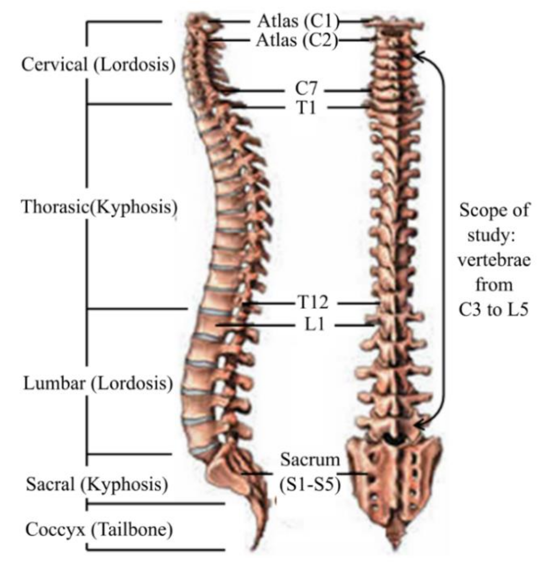
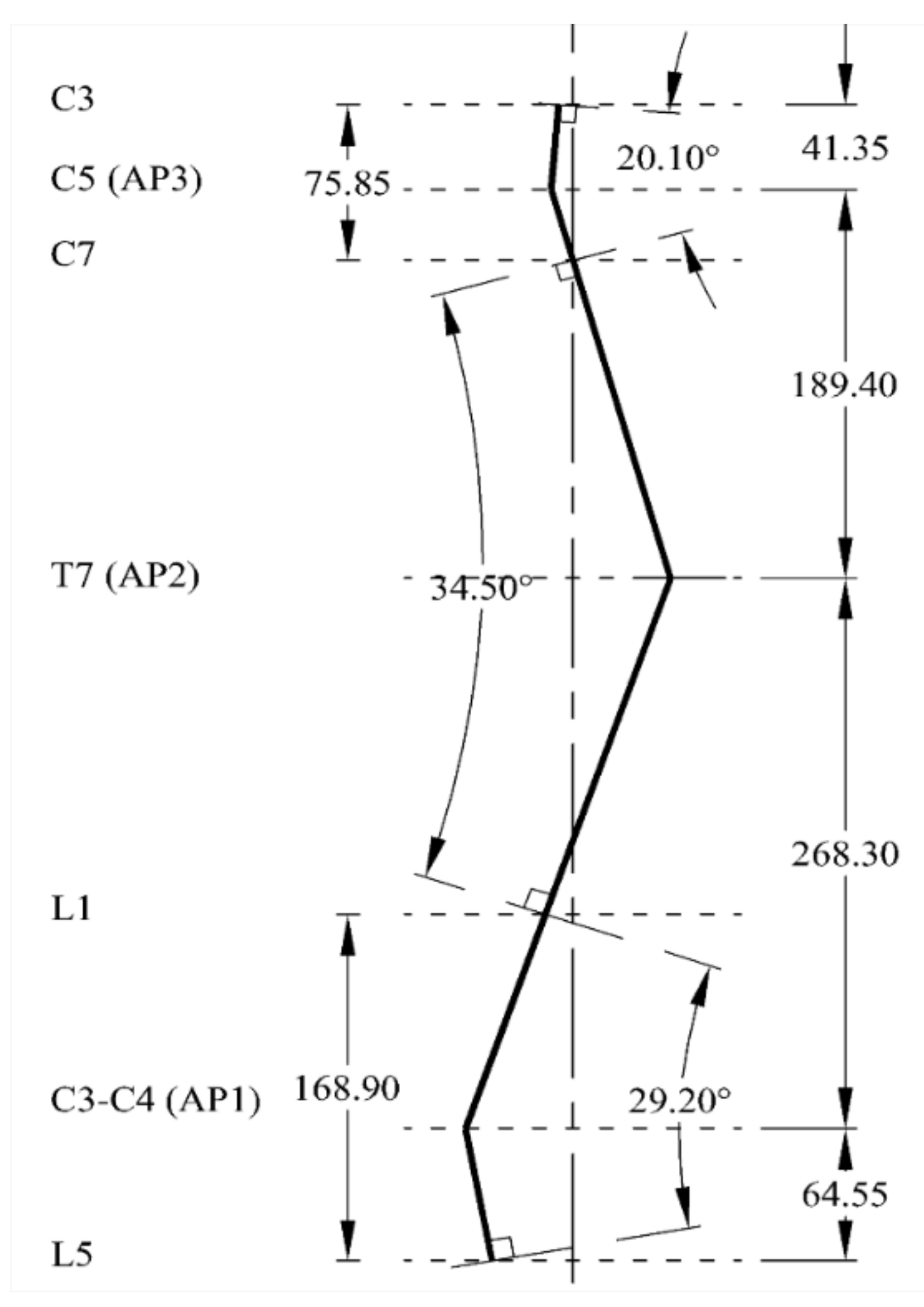
2. Geometrical Input of Spine

The geometrical input data for the generation of spine biotensegrity models were gathered from the anatomical parameters of human spines by Busscher, et al. [24] where the human spine specimens were collected from six male cadavers with age and body height at death ranging from 55–84 year-old and 175–192 cm, respectively (mean of 72 year-old and 182cm, respectively).

2.1. Vertebrae Anatomical Parameters

Figure 2 shows typical vertebrae in superior and lateral views whereas Figure 3 shows a typical human spine in sagittal and posterior views. Sagittal and posterior views are medical terms that refer to the appearance of the spine when viewed from the side and behind, respectively. Figure 3 shows a total of twenty-two vertebrae from the cervical (vertebrae C3,C7), thoracic (vertebrae T1T12) and lumbar regions (vertebrae L1–L5) that were considered in this study. Anatomical parameters such as the vertebral end-plate width denoted as EPW (mean value of upper and lower vertebral end-plate width denoted as UEPW and LEPW, respectively), vertebral central body height denoted as VBHC and intervertebral disc height denoted as IDH from the source by [24] were considered in the generation of the spine biotensegrity models.

2.2. Natural Sagittal Curvature

The human spine (Figure 3) has a natural curvature in sagittal view with: (i) lordosis (concave curve) at cervical and lumbar regions and (ii) kyphosis (convex curve) at thoracic and sacral regions. According to Busscher, et al. [24], cervical lordosis of 20.1°, thoracic kyphosis of 34.5° and lumbar lordosis of 29.2° were measured as the angles between the upper end-plate of C3 and the lower end-plate of C7, the upper end-plate of T1 and the lower end-plate of T12 and the upper end-plate of L1 and the lower end-plate of L5, respectively. These angles are reasonably accepted and supported by others. For instance, the fact that thoracic kyphosis lies between 20–45° has been suggested by Mejia, et al. [25]. Been and Kalichman [26] have reported a normal range of 30–80° for lumbar lordosis.

The apex of the curvature is defined as the farthest point of a vertebra from the C7 plump line. The C7 plumb line is established by extending a vertical line from the center of C7 vertebral body to the posterior corner (at the back) of sacrum S1 [28]. The normal weight of the human body generally acts through the C7 plumb line. Nevertheless, there are insufficient anatomical data about sacrum S1 in the study by Busscher, et al. [24]. Hence, an assumption that the C7 plumb line rests on the right end of the vertebrae L5 adjoining to S1 was made in this study.

Figure 4 shows the established natural sagittal line for the spine biotensegrity models. It is noted that there is an apex each within cervical lordosis, thoracic kyphosis and lumbar lordosis in a human spine. The decision on the location of these apexes is based on several pieces of literature. The apex of lumbar lordosis, AP1, is assumed at the intervertebral disc between L3-L4 whereas the apex of thoracic kyphosis, AP2, is assumed at vertebrae T7 [29]. The apex of cervical lordosis, AP3, is assumed at C5 according to Knox and Lonner [30], who suggested the lordotic climax in between C4–C6. One of the most common methods, namely the Cobb method, has been adopted in establishing the curvature of the spine biotensegrity model. A review on this method can be found in [31].

3. Search Strategies for Spine Biotensegrity Models

This section presents the key steps in the search strategies for spine biotensegrity models: (1) the generation of geometrical model, and (2) the formulation of mathematical equations.

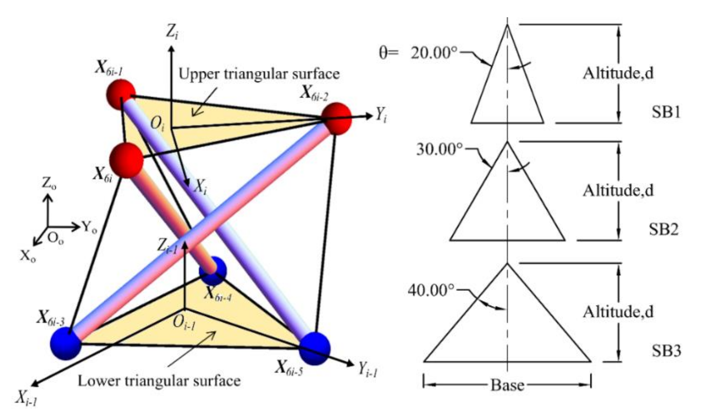
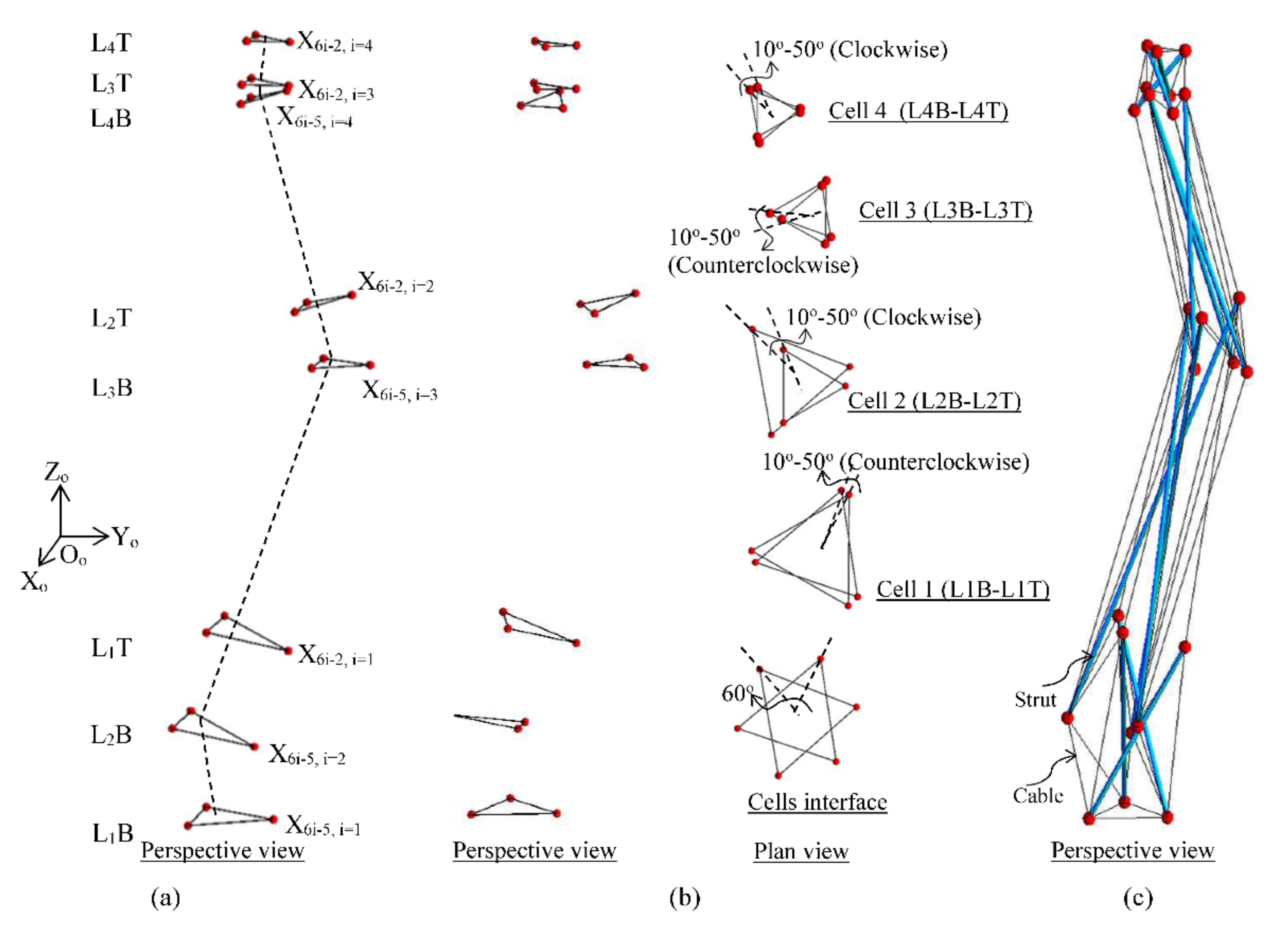
3.1. Geometry of the Spine Biotensegrity Model

The geometry of the spine biotensegrity model was defined by their nodal information, which is described in the basic cell such as the triangular cell and element connectivity.

3.1.1. Definition of Basic Cell

The triangular cell has been chosen to mimic the human spine, due to its simplicity of application. Figure 5 shows the definition of a typical triangular cell and triangular surfaces of the spine biotensegrity models. A total of three variations of spine biotensegrity models identified as SB1, SB2, and SB3, with different sizes of triangular cells have been proposed in this study. The geometry of a triangular cell is presented in the global Cartesian coordinate system O_o-X_oY_oZ_o. The position vector of nodal coordinates is denoted as X. The origins of the local Cartesian system O_{i – 1}-X_{i - 1}Y_{i - 1}Z_{i - 1} and O_i-X_iY_iZ_i are positioned at the centroid of lower (X_6i-5 X_6i-4 X_6i-3) and upper triangular surfaces (X_6i-2 X_6i-1 X_6i) of ith (i = 1, 2, …, n) triangular cell, respectively.

The nodal coordinates in plane XY of the spine biotensegrity models are determined based on triangle altitude, d and half of the vertex angle, θ of the lower and upper triangular surfaces in the local Cartesian system. The tapered section properties of a human spine are incorporated into the spine biotensegrity models (the width of vertebra gradually increases from cervical vertebrae to lumbar vertebrae). Reference is made to the EPW of vertebrae to characterize the widths of the spine biotensegrity models and these widths are adopted as the triangle altitudes for the triangular surfaces in cells.

It is noted that all spine biotensegrity models have the same magnitude of triangle altitude (d) (see Figure 5). SB1, SB2, and SB3 are different in terms of half of the triangle vertex angles (θ) with values of 20°, 30°, and 40°, respectively. While accumulation of both VBHC and IDH represents the height of the spine biotensegrity model, accumulation of IDH represents the saddle height between two independent cells.

3.1.2. Definition of Basic Cell

Tensegrity are classified into class one, two and k depending on the numbers of strut at a node [32]. In this study, class one tensegrity mast is chosen for the spine biotensegrity models to mimic the stacking up of discontinuous compressive vertebral bodies of a human spine. Specifically, class one tensegrity mast consists of struts (i.e., vertebrae) that are connected solely by cables (i.e., muscles, intervertebral disc) and offers no contact in-between the struts, such as a human spine (i.e., vertebrae are cushioned by intervertebral disc and surrounded by muscles).

Figure 6 shows the developed element connectivity chart inspired by Pugh’s illustration of the diamond pattern. The N-stage class one spine biotensegrity models with N triangular cells are assembled according to the chart. The element connectivity at the second and third stage may be repeated in order to stack up to n triangular cells. The lower and upper triangular surfaces of ith (i = 1, 2, …, n) triangular cell are denoted as L_iB and L_iT, respectively. The triangular cell that is stacked up on the current ith triangular cell is denoted as the (i + 1)th cell. All the elements are classified into specific groups. The struts in every stage are represented by bold lines. The saddle cables (red color) connecting the interface between two triangular cells are represented by irregular dash-dotted lines. Horizontal cables in regular dashed lines join the nodes only at the base and the top of the structures. There are three categories of diagonal cables; namely diagonal cables 1 (cyan color) connecting nodes L_iB and L_{i + 1}B, diagonal cables 2 (pink color) connecting nodes L_iT and L_{i + 1}T, and diagonal cables 3 (blue color) connecting nodes L_iB and L_iT. On top of that, reinforcing cables in zig-zag lines at the first stage are also included.

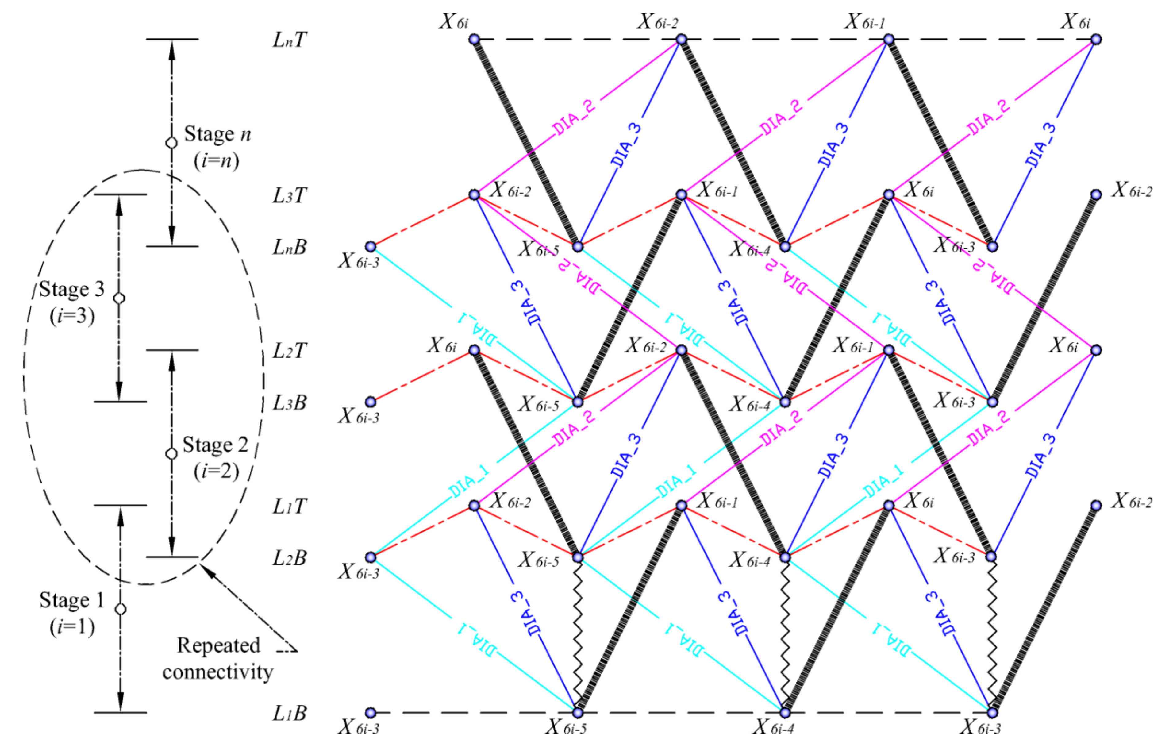
3.1.3. Assemblage of Spine Biotensegrity Models

As mentioned earlier, a total of three variations of spine biotensegrity model, namely SB1, SB2 and SB3 are developed. These three four-stage spine biotensegrity models are proposed based on the nature of three apexes in a human spine.

Figure 7 shows the assemblage process of a spine biotensegrity model with four triangular cells. Firstly, major positions of the eight triangular surfaces for the four triangular cells are decided. The triangular surfaces are placed as follows: one at the base, two at each of the apex and one at the top. The altitudes of the triangular surfaces at each stage are based on the anatomical parameter EPW at the respective height of the human spine specimens. The altitude of triangular surfaces decreases along with the height until the top of the spine biotensegrity model to change accordingly.the taper-form and slenderness of a human spine. These triangular surfaces are then aligned perpendicular to and have their centroids coinciding with the established curvature line as shown in Figure 4. Note that, nodes X_6i-5 and X_6i-2 of ith triangular cell (Figure 5) are positioned on global Y axis (x = 0), prior to the twisting process (Figure 7a).

Next, the triangular surfaces are rotated so that all the triangular cells have an initial twist angle in the range of 10° to 50° in clockwise and counterclockwise for odd- and even-number of ith triangular cell, respectively (Figure 7b). Furthermore, the rotational angle between the triangular surfaces forming the interface of two triangular cells is set at 60° with the same rotational direction as the twisting direction of the lower cell.

Lastly, the triangular surfaces are removed except for their nodes at the established positions. The generation of the spine biotensegrity model is complete after the placement of all the struts and cables according to the developed element connectivity pattern as shown in Figure 6 (Figure 7c). Each spine biotensegrity model consists of sixty-nine elements (i.e., twelve struts and fifty-seven cables). The following section presents the formulation of the equations for the search of the self-equilibrated state of a spine biotensegrity model.

3.2. Equilibrium Equations of Spine Biotensegrity Model

This study is aimed at establishing the feasible self-equilibrium configuration for four-stage class one spine biotensegrity models by the means of form-finding analysis.

3.2.1. Basic Assumptions

Form-finding of four-stage class one spine biotensegrity models that are stabilized by prestresses at the self-equilibrated state is carried out. The following assumptions are made for form-finding analysis:

• Self-weight of struts and cables are neglected due to the reason that the stress resulted from self-weight is insignificantly small compared to the level of pre-stress [19].
• There is no external force acting on the models. It is necessary to ensure the self-equilibrium position as shown under the topology of biotensegrity model (Figure 7) is rational. Against any disturbance, the self-equilibrium and stability of the obtained topology should be retained. Analysis to study the capability of the established spine biotensegrity to undergo change in shape is not the scope of the study.

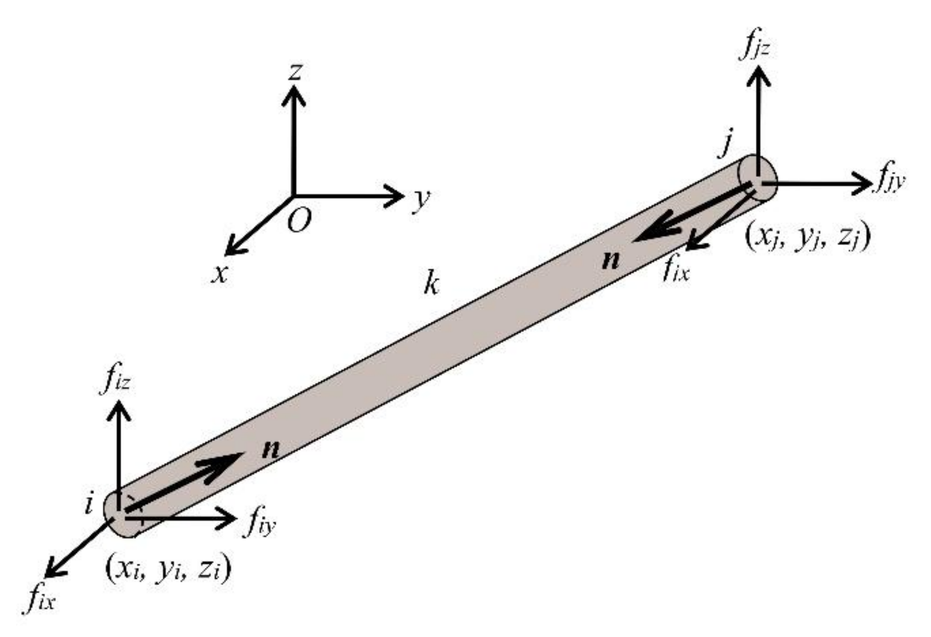
3.2.2. Equilibrium Equations: Formulation

As the spine biotensegrity model consists of struts and cables that are pin and connected, the set of equilibrium equations adopted in this study is derived based on the basic formulations of pin-jointed structures. Such formulation for tensegrity structures can also be found in [32,33].

The spine biotensegrity model in this study consists of m elements, n_o nodes, n_c supports and n_u = 3(n_o-n_c) unconstrained degree of freedoms. Consider an element k of the spine biotensegrity model connecting node i and j (i < j) in a Cartesian coordinate system O-XYZ as shown in Figure 8. The vectors of nodal coordinates of node i and j are denoted as ${\stackrel{-}{\mathrm{x}}}_i$ and ${\stackrel{-}{\mathrm{x}}}_j$, respectively.

The length of element k is evaluated using the following expression:

$$L_T=\sqrt{{\left(x_j-x_i\right)}^T\left(x_j-x_i\right)}$$

(1)

The vector of directional cosines λ of an element k is defined as follows:

$$\lambda =\frac{\left({\mathit{x}}_j-{\mathit{x}}_i\right)}{L_T}$$

(2)

Figure 8 also shows the axial force n of element k for the spine biotensegrity model, and the components of the nodal force at i and j, f_i and f_j, respectively (where f_i = - f_j), which are in equilibrium with n. Considering equilibriums at all nodes, the following equation can be obtained:

$$F=Bn$$

(3)

where B is a n_u × m matrix consisting of the vector of directional cosines λ of all elements in the spine biotensegrity model with respect to x, y, z axes, F is a vector of nodal forces with size n_u and n is a vector of axial forces for all elements with size m.

By making use of the Moore–Penrose generalized inverse, the necessary and sufficient condition for the existence of solution for Equation (3) can be expressed using the following equation:

$$F=B{B}^{+}F$$

(4)

which can be rewritten in the following form

$$[I_{n_u}-B{B}^{+}]F=0$$

(5)

where $I_{n_u}$ is an identity matrix of order n_u and B⁺ is Moore–Penrose generalized inverse of matrix B. Singular value decomposition method is used in this study to compute the Moore–Penrose generalized inverse of the matrix B with rank deficiency (i.e., rank < n_u).

For the case of self-equilibrated state without external forces, F = 0. Under such condition, the solution for the vector of axial forces n for the spine biotensegrity model is given by the following equation:

$$n=[I_m-B^{+}\mathbf{{\rm B}}\mathbf{]}\mathsf{\beta }$$

(6)

where β is a vector of arbitrary coefficient of size m.

Denoting matrix [I_m− B⁺B] in Equation (6) as matrix G of size m × m and applying eigenvector basis decomposition method, the real symmetric matrix G can be expressed as follows:

$$G=\Phi \Lambda {\Phi }^T$$

(7)

where Λ is a diagonal matrix whose diagonal elements Λi (i = 1, 2,…, m) correspond to eigenvalues of matrix G; Φ is an orthogonal matrix whose ith column Φ _i (i = 1, 2,…, m) corresponds to eigenvector associated with eigenvalue Λi. Since matrix G is an orthogonal projection matrix, the eigenvalues Λ_i returns the value of either 0 or 1. The eigenvectors Φ_i correspond to vectors of independent self-equilibrium stress modes for biotensegrity models considered in this study. It is noted that the number of vectors of independent self-equilibrium stress modes is equal to the number of non-zero eigenvalues of matrix G or rank [G].

Substituting Equation (7) into Equation (6) and then multiplying both sides of the resulting equation with Φ _i ⁻¹ as follows:

$${\Phi }^{-1}n={\Phi }^{-1}\Phi \Lambda {\Phi }^T\mathsf{\beta }$$

(8)

the following expression for vector of axial forces n can be obtained:

$$n=\Phi \Lambda \mathsf{\beta }*$$

(9)

where β * = Φ^Tβ.

Assuming that the spine biotensegrity model has q number of independent self-equilibrium stress modes, Equation (9) can be further rewritten as

$$n={\displaystyle \sum _{i=1}^q{\beta }_i{}^{*}{\Phi }_i}$$

(10)

where β_i* is ith component of vector β*, which corresponds to vector of coefficients for the linearly independent self-equilibrium stress modes.

Equation (10) shows that the solution of vector of axial force n is dependent on the choice of the combinations of coefficients β_i*, which might be more than one. In this study, only one of the possible combinations of coefficients β_i* was used to determine the vector of axial forces n.

3.2.3. Equilibrium Equations: Solutions

In this study, the spine biotensegrity model is found to have three independent self-equilibrium stress modes (q = 3). In order to find the possible linear combination of the three self-equilibrium stress modes, an iterative procedure is adopted in this study. Two main steps are involved in the iterative steps. The first one is the determination of trial set of coefficients β_i* for an assumed configuration of spine biotensegrity model. The other is the modification of the assumed configuration until one consistent self-equilibrated configuration is found. For the determination of the trial set of β_i*, an unconstrained minimization problem as shown in Equation (11) is adopted where the conjugate gradient method is used:

$$\min f(x)=-{\beta }_1^{*}\times {\beta }_2^{*}\times {\beta }_3^{*}$$

(11)

Equation (11) is an objective function to prevent excessive axial forces. The set of β_i* (i = 1,2,3) determined by solving Equation (11) is used as the trial values to determine the possible solution for n (see Equation (10)), which satisfies the inequality constraints given in Equations (12) and (13) using an iterative process:

$$0\le n_c\le {\sigma }_c{A}_c$$

(12)

$$-\frac{{\pi }^2{E}_s{I}_s}{l_s{}^2}\le n_s\le 0$$

(13)

where n_c, E_c and A_c are axial forces, yield stress and cross sectional area for cable elements, respectively; n_s, E_s, I_s, L_s, σ_s and A_s are axial forces, Young modulus, moment inertia of section, length, yield stress and cross sectional area for strut elements, respectively. In this study, A_c = 3.14 mm², A_s = 50.30 mm², E_s = 200 GPa, and I_s = 201 mm⁴.

As shown in Equations (12) and (13), in addition to checking against yielding of cable elements, compressive forces of strut elements are checked against Euler’s buckling load. The applied inequality constraints ensure that the axial forces for all the cable and strut elements are within their upper bound axial force limits and satisfy the elastic condition of the material properties.

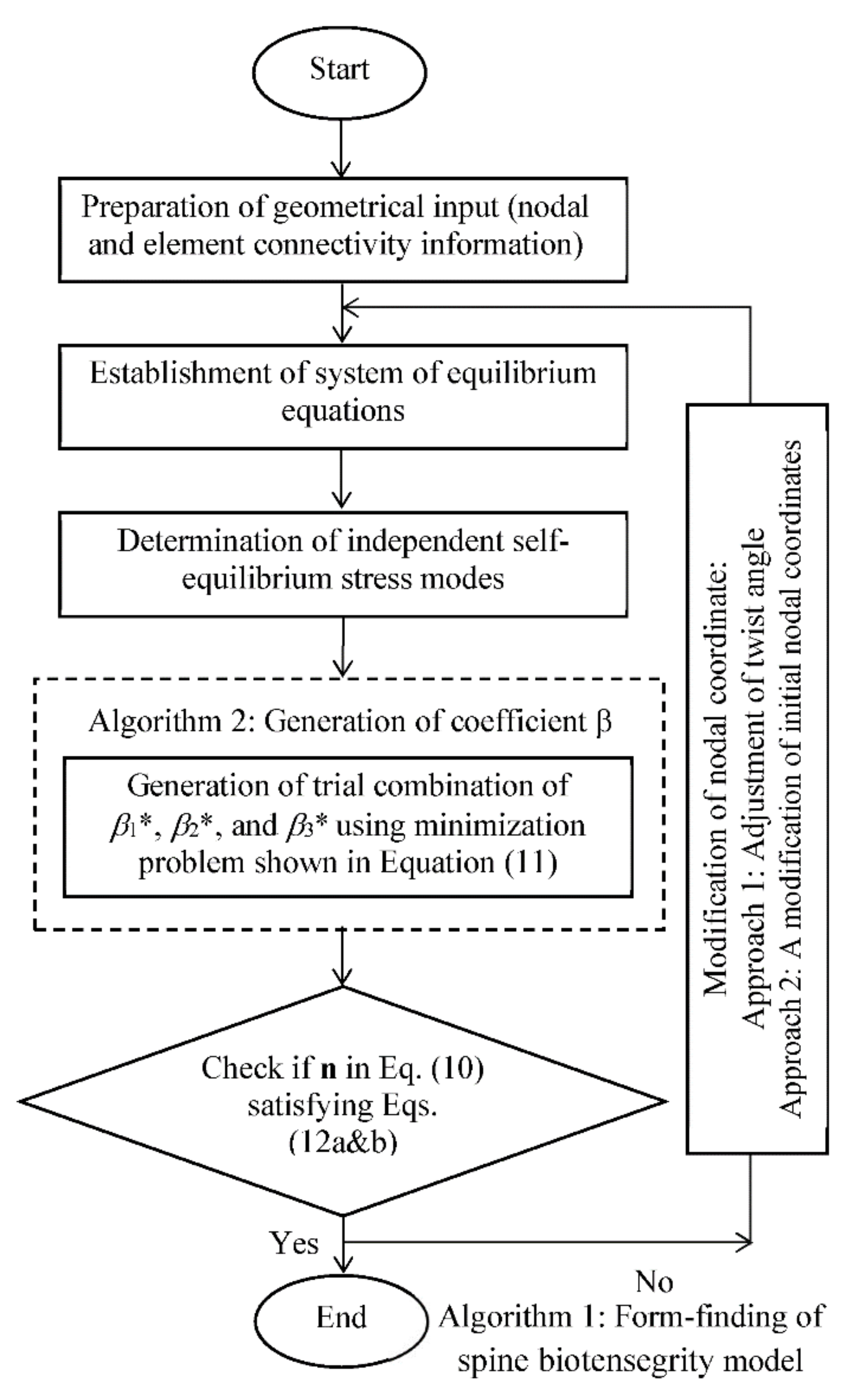
3.3. Algorithm for Form-Finding of Spine Biotensegrity Model

The flowchart in Figure 9 summarizes the strategies to search for a possible self-equilibrated state of the spine biotensegrity model. Algorithm 1 begins with the preparation of geometrical input of the spine biotensegrity model in the form of four-stage class one tensegrity mast with triangular cells. A spine biotensegrity model is generated with the application of initial twist angles to each triangular cell. The angles may be considered as the anatomical parameters. Vector of axial forces n satisfying self-equilibrium condition, as shown in Equation (10), is established. The eigenvector basis decomposition method is adopted to determine the independent self-equilibrium stress modes.

Algorithm 2 is the subset of Algorithm 1 and provides an initial estimate for coefficients β_i* through the minimization problem as shown in Equation (11). It is noted that the combination of coefficients β_i* is searched through an iterative form-finding process to satisfy the Equations (12) and (13). After obtaining the combination of the coefficients β_i*, the substitution of the coefficients β_i* into Equation (10), gives the axial forces n in the self-equilibrium state.

The form-finding strategy for searching the self-equilibrated models is studied through two approaches. Under approach one (Figure 10a), different combinations of twist angles are applied to a group of basic cells of a trial spine biotensegrity model. Under approach two (Figure 10b), unconstrained nodal coordinates of a trial spine biotensegrity model are modified through a relatively small magnitude (2% of the height of spine biotensegrity model in this study). Design valuables are coefficients β_i* and nodal coordinates. As the objective function and the constraint conditions cannot be explicitly expressed by design variables, the procedure of form-finding implies an iteration. Both approaches involve only minor modification of nodal coordinates due to the priority of searching for models with close resemblance to the geometry of the human spine.

4. Search Results for Spine Biotensegrity Models

The process of finding the possible self-equilibrated state of spine biotensegrity models using the iterative approach (Figure 9) is presented. Specifically, the results of the processes through approaches one and two whereby number of slackened cables in compression (slackened cables) are continuously reduced and eventually eliminated in order to achieve self-equilibrated configuration of spine biotensegrity model are presented. Due to the similar process, only spine biotensegrity model SB1 was chosen to demonstrate the form-finding approaches.

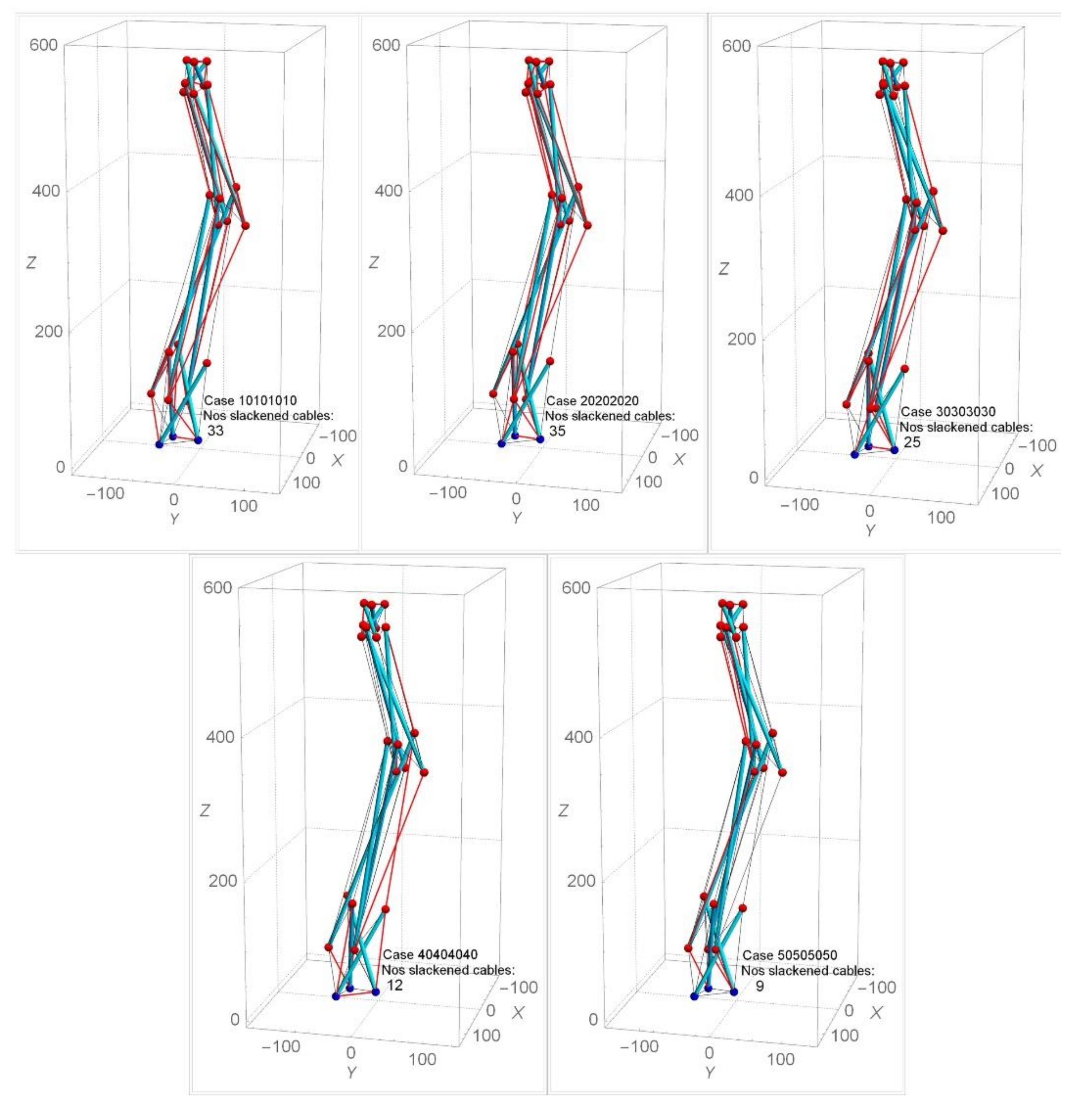
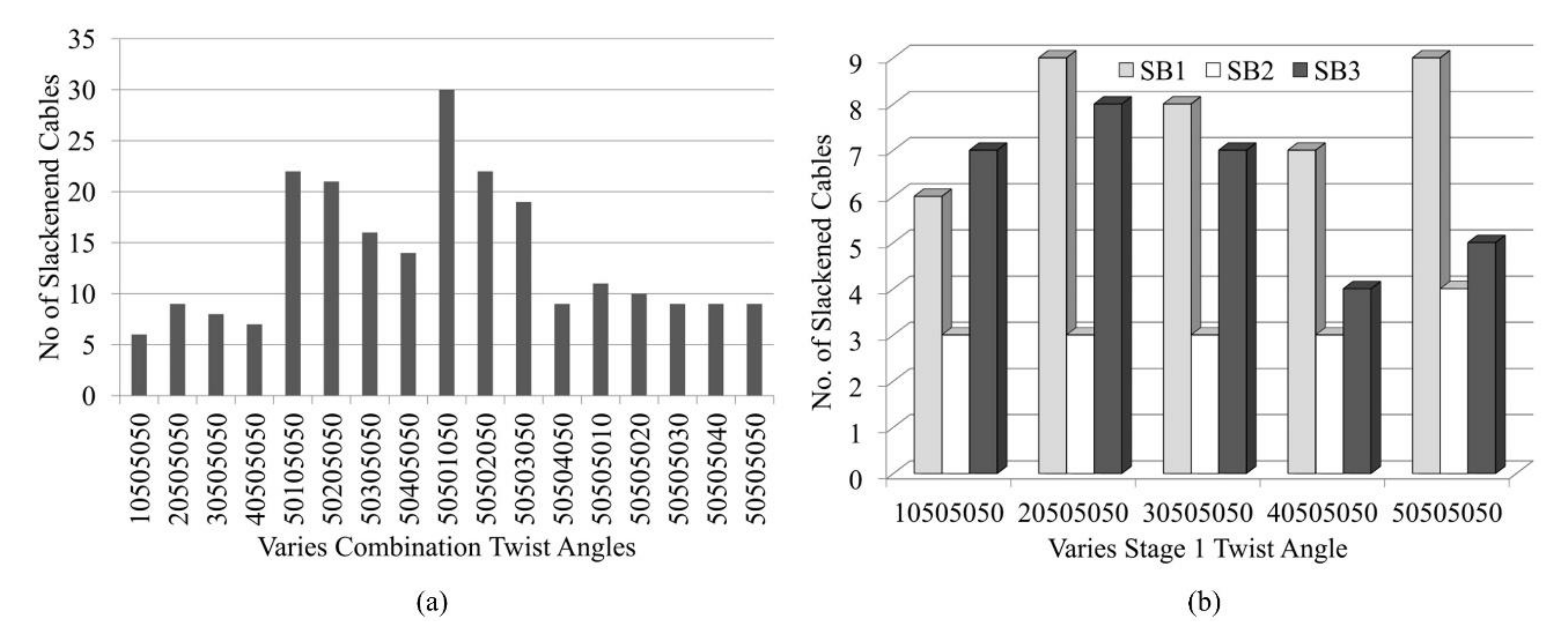
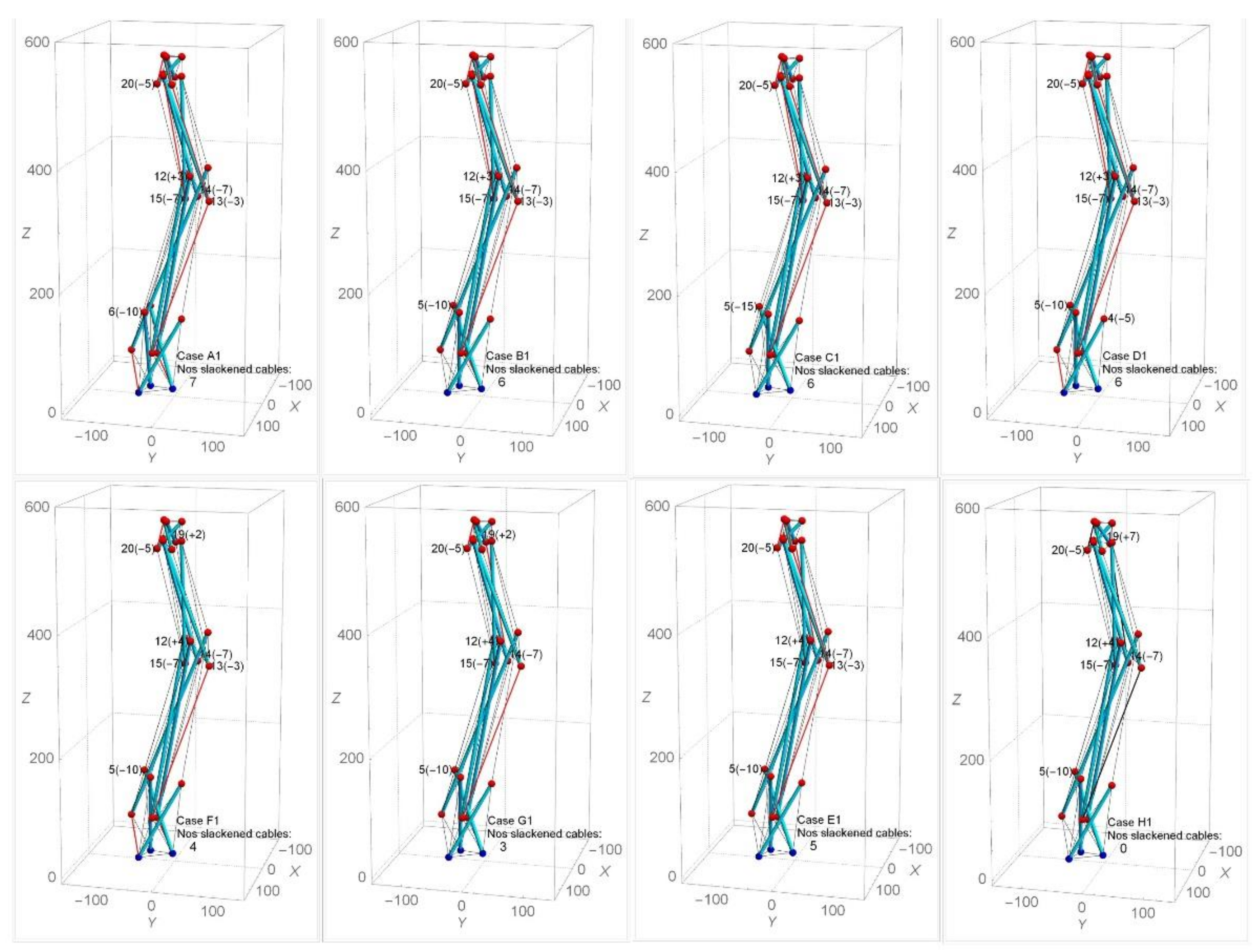
4.1. Analysis Results Using Approach One

Under approach one, a random choice of each stage’s twist angle ranging from 10° to 60° has been selected for the form-finding analysis for the spine biotensegrity models. The symbol α_i is defined by the twist angles for the i-th stage’s triangular cells. Arrangement of the spine biotensegrity models with α_i $\ge$ 60° is found to be not feasible due to the problem of closely spaced struts. Figure 11 shows the form-finding analysis with the application of the same twist angle 10° to 50° for all the triangular cells in the spine biotensegrity models (i.e., cases 10101010, 20202020, 30303030, 40404040, and 50505050). The case 10101010 denotes the model as α₁=α₂ = α₃ = α₄ = 10°. The cables in compression are slacked and should be removed. The slackened cables of SB1 are indicated by the red line (Figure 11). From the form-finding analysis, it is found that SB1 with α₁ = α₂ = α₃ = α₄ = 50° yields the least degree of slackness (9 slackened cables). Larger twist angles tend to reduce the number of slacked cables, but at α₁ = α₂ = α₃ = α₄ = 20°, the number of slacked cables is maximum. For 10° $\le$ α_i $\le$ 40°, slackened cables are found to occur throughout the model. For α_i = 50°, more slackened cables are found to occur at the first and third stages. The information about slackened cables at each trial case is an important input in the iterative analysis.

Figure 12 shows the analysis with the application of various combinations of twist angles for triangular cells within the model (i.e., cases 10505050, 20505050, 30505050, and 40505050). It is found that cases where the α₁ for the triangular cell at stage 1 is less than 50° lead to a lesser number of slackened cables in comparison with other combinations of α₂, α₃, α₄ (Figure 12a). A similar effect of such combinations of twist angles is found in SB2 and SB3. When α₁ changes while the other α_i are held at 50°, the numbers of slackened cables ranged from three to nine for SB1, SB2, and SB3 are found (Figure 12b). In the model SB1 and SB3, the numbers of slackened cables are maximum at α₁ = 20°. In the case of α₁ = 10^o in SB1 and α₁ = 40° in SB3, the number of slackened cables is minimum. On the other hand, SB2 is not sensitive to α₁. In SB1, as α₂ and α₃ are assigned larger values, the number of slackened cables decreases. Figure 13 illustrates the numbers and position of slackened cables for parameter α₁ = 10°−40° and α₂ = α₃ = α₄ = 50° in SB1. At α₁ = 10°, number of slackened cables decreases to five and is uniformly located throughout the stages.

4.2. Iterative Results Using Approach Two

Self-equilibrated state of spine biotensegrity models cannot be found by approach one. The case 30505050 (selected based on the form-finding results from SB1, SB2 and SB3) is then employed in approach two in the subsequent process of searching for the self-equilibrated configuration. Under approach two, the modified nodes are 18 nodes excluding the base and top nodes (i.e, node 4 to node 21). The controllable range of the nodal coordinates is less than 15 mm in the y direction. Few cases (i.e., cases A1 to H1) that are close to the self-equilibrated state are chosen to demonstrate the feasibility of the form-finding approach. Figure 14 shows the numbers and positions of slackened cables in SB1. It is seen that SB1 still preserves the spine anatomical parameters, especially the natural curvature of the spine. It is also important to note that the position of slackened cables changes even though the modifications of nodal coordinates are small.

Table 1. Axial forces in SB1 for cases A1–H1.

Modification of Nodal Coordinates (mm) in Y-Direction for Cases A1-H1
Case	Nodes													Case	Nodes
	6	20		15	12		13	14		5		4	19		6		20	15		12	13		14	5		4	19
A1	−10	−5		−7	3		−3	−7		0		0	0	E1	0		−5	−7		4	−3		−7	−10		0	0
B1	0	−5		−7	3		−3	−7		−10		0	0	F1	0		−5	−7		4	−3		−7	−10		0	2
C1	0	−5		−7	3		−3	−7		−15		0	0	G1	0		−5	−7		4	0		−7	−10		0	2
D1	0	−5		−7	3		−3	−7		−10		−5	0	H1	0		−5	−7		4	0		−7	−10		0	7
Axial Force (N) for Case 30505050 and Cases A1-H1
Cable			30505050			A1			B1		C1			D1		E1			F1			G1			H1
40			−7.73			1.65			3.94		10.00			10.00		5.00			10.00			5.00			6.07
42			10.00			−2.74			0.11		1.58			−2.24		1.93			−7.74			1.85			0.79
50			−8.82			18.54			13.10		17.25			18.81		13.31			13.63			10.88			3.82
51			−1.11			−2.27			−2.77		−4.06			−3.73		−5.45			−4.13			−4.44			0.03
57			−28.56			−2.52			−1.69		−1.44			−2.10		8.42			12.57			14.38			22.26
58			12.93			−8.27			−8.49		−12.13			−11.63		−5.71			0.45			6.28			30.40
59			−6.35			0.43			0.68		0.93			0.85		−0.59			0.16			−1.07			4.27
65			−5.27			−13.28			−9.38		−12.76			−13.66		−14.13			−11.70			−12.91			0.03
66			10.00			−5.29			−5.64		−8.06			−7.67		−3.06			1.97			5.88			24.13
67			−2.89			−1.41			−0.81		−0.10			0.05		0.13			−0.60			0.03			0.03
68			−7.86			10.00			6.65		10.91			11.04		2.91			10.00			3.09			6.57

Note: Shaded cells denote slackened cables.

presents the axial forces of the potential slackened cables of SB1. As can be seen in Table 1, although the slackened cables 40, 50, 59, and 68 may change into tension state easily, the remaining cables (particularly cable 51 and 65) remain slackened in most of the cases. In the case of B1, it is apparent that the case with the modification of node 5 instead of node 6 reduces the degree of slackness in most of the slackened cable (especially in cables 40, 42, 57, 65, and 67). Additionally, the modification of node 19 in case F1 clearly shows the effect of further reducing the degree of slackness in the slackened cables 51, 59, 65, and 66 compared to case E1. However, such modification in case F1 also leads to an increase in the degree of slackness in slackened cables 42 and 67. This situation is improved by excluding node 13 in case G1. Since node 19 showed its significance in changing slackened cables 51, 59, 65, and 66 to tension state, further modification of coordinates of node 19 was carried out. This led to case H1, where a self-equilibrated SB1 is successfully determined. Similar form-finding strategies are applied to SB2 and SB3.

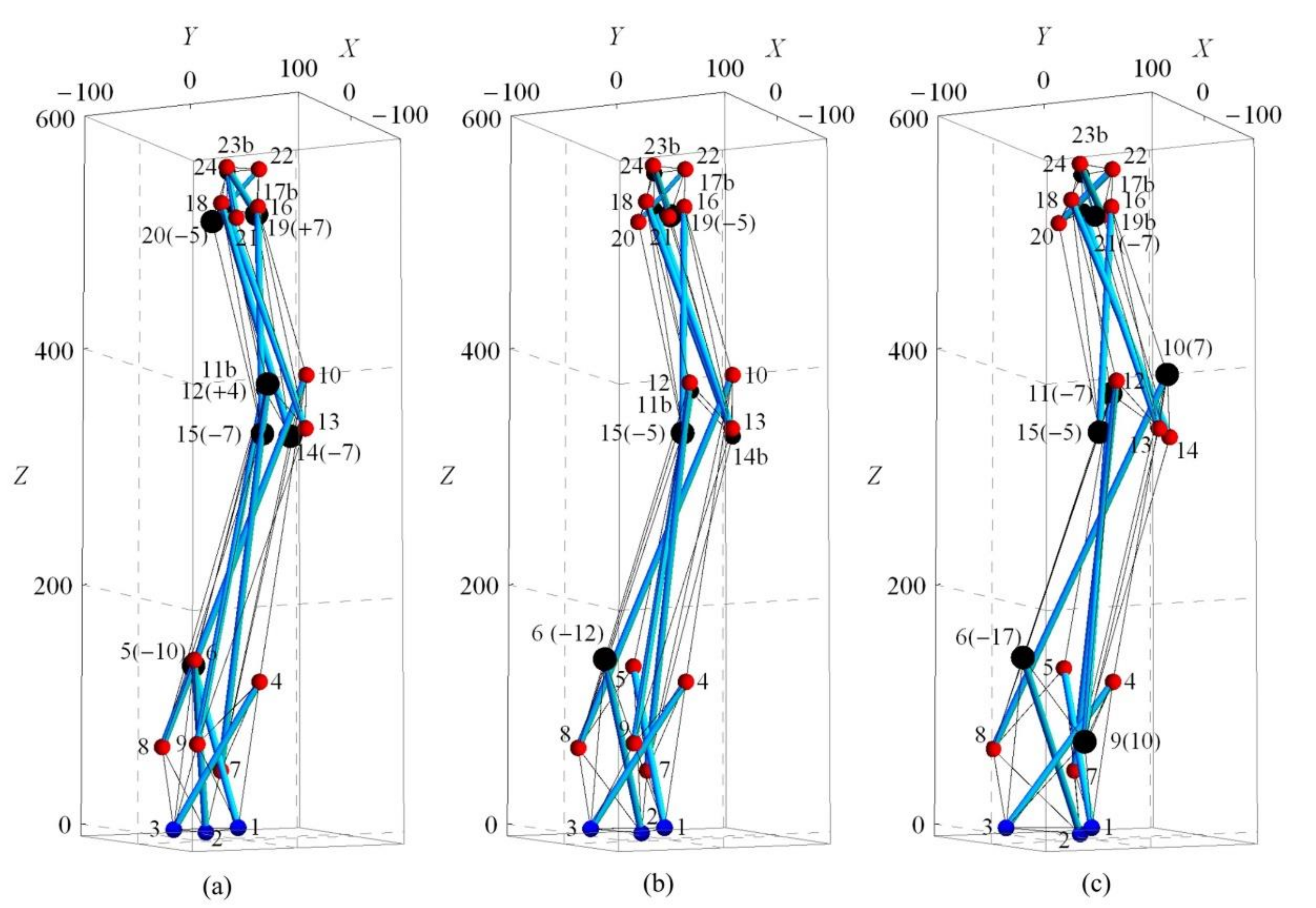
4.3. Spine Biotensegrity Models

Three variations of spine biotensegrity models (SB1, SB2, and SB3) are successfully established by using the proposed form-finding strategies. Figure 15 illustrates the configuration and nodal numbers. The larger nodes represent the modification through approach two. In any model, nodes of all cells excluding the nodes at top and base are considered for modification during approach two.

Table A1. Nodal coordinates of SB1, SB2 and SB3.

Nodes	SB1			SB2			SB3
	x	y	z	x	y	z	x	y	z
1	9.33	−1.23	0	9.33	-1.23	0	9.33	−1.23	0
2	−24.01	−48.3	0	−35.34	−45.27	0	−49.24	-41.54	0
3	14.67	−58.67	0	26	−61.7	0	39.91	−65.43	0
4	−8.9	9.49	123.78	−8.9	9.49	123.78	−8.9	9.49	123.78
5	−14.71	−55.48	141.36	−25.95	−48.49	141.36	−39.72	−52.18	141.36
6	23.61	−35.21	141.36	34.85	−44.2	141.36	48.62	−45.51	141.36
7	−33.22	-39	52.83	−33.22	−39	52.83	−33.22	−39	52.83
8	11.48	−71.52	70.41	8.47	−82.75	70.41	4.77	−96.53	70.41
9	21.75	−33.19	70.41	24.76	−21.96	70.41	28.45	1.82	70.41
10	−10.04	52.87	382.82	−10.04	52.87	382.82	−10.04	59.87	382.82
11	−7.19	14.89	372.81	−14.34	11.56	372.81	−23.12	0.46	372.81
12	17.23	30.28	372.81	24.38	29.61	372.81	33.16	33.7	372.81
13	14.15	63.71	332.85	14.15	63.71	332.85	14.15	63.71	332.85
14	−18.11	34.13	332.85	−24.57	45.65	332.85	−32.51	51.21	332.85
15	3.96	18.67	332.85	10.42	16.15	332.85	18.36	10.49	332.85
16	−5.08	10.05	531.04	−5.08	10.05	531.04	−5.08	10.05	531.04
17	−7.84	−21.15	533.31	−13.91	−22.77	533.31	−21.37	−24.77	533.31
18	12.91	−15.59	533.31	18.99	−13.96	533.31	26.44	−11.96	533.31
19	−18.29	2.21	527.57	−18.29	−9.79	527.57	−18.29	−4.79	527.57
20	6.37	−27.52	519.59	4.74	−28.59	519.59	2.74	−36.05	519.59
21	11.93	−1.77	519.59	13.56	4.31	519.59	15.55	4.77	519.59
22	−7.58	9.77	564.29	−7.58	9.77	564.29	−7.58	9.77	564.29
23	−5.12	−18.78	564.29	−10.33	−21.21	564.29	−16.74	−24.21	564.29
24	12.7	−10.47	564.29	17.91	−8.04	564.29	24.33	−5.05	564.29

in Appendix A shows the nodal coordinates for the spine biotensegrity models.

The determined coefficients β_i are −1399.907, −2490.990, −131.972 in SB1, 786.626, −2855.643, 462.793 in SB2 and −1368.241, 1188.504, 74.294 in SB3. The above sets of coefficients beta β_i (i = 1, 2, 3), are used to calculate the vector of axial forces (see Equation (10) that satisfy the inequality constraint represented by Equations (12) and (13). It is emphasized that the solution obtained for the self-equilibrated configuration for SB1, SB2, and SB3 represents one possible configuration with close resemblance to the geometry of the human spine. The self-equilibrated configuration could be further refined through solution of constrained optimization problem using maximum stiffness, minimum weight or other suitable criteria as objective functions.

In the process of determination of coefficients β_i*, the combinations of coefficients β₁*, β₂* and β₃* that lead to tension in struts or compression in cables are rejected. Non-acceptance of the trial values of coefficients β_i*(i = 1,2,3) obtained from solution of problem defined by Equation (11) is always due to non-satisfaction of Equation (12) (the existence of slackened cables) within the trial configuration of spine biotensegrity models.

The proposed form-finding strategy using approach one and two yields updated trial configurations of spine biotensegrity models to reduce slackened cables and to maintain closely the geometrical characteristics of the spine. Approach two eliminates inconsistent cables and further refines the configuration. It is found that, although modification of nodal coordinates in some cases can reduce slackened cables, increment in the degree of slackness in other slackened cables and the generation of new slackened cables are observed. Therefore, a good understanding of the relationship between the modified nodes and the change in axial forces in a spine biotensegrity model is essential in searching for a self-equilibrated model.

5. Conclusions

This paper presents a trial-and-error iterative process for form-finding of three variations of biotensegrity models inspired by the form of human spine. The developed element connectivity chart inspired by Pugh’s diamond pattern is able to generate N-stage class one biotensegrity structures. The proposed form-finding strategy consists of two approaches. In the first approach, the twist angles of the cells in each stage, which simulates the geometrical characteristics of the spine, are varied to reduce slackened cables. In the second approach for further refinement, nodal coordinates are varied to reduce and eliminate slackened cables. Through form-finding analysis, the characteristics of the biotensegrity models are found. Twist angle, except for the lowest cell, are appropriate at 50^o. The slacking of cables is very sensitive to twist angles near the thoracic and lumbar region. The sensitivity to twist angle of the lowest cell is dependent on the shape of the cell. This study has successfully established for the first time the possible self-equilibrated configurations of biotensegrity models inspired by the human spine. Future works such as shape change analysis, building and controlling real biotensegrity models and conducting experiments considering external loading and operational challenges as well as formulation of self-collision and external collision of the spine biotensegrity models should be carried out. The outcome of such future works could then lead to the possible application of spine biotensegrity in area of robotic tools and deployable structures.

References

1. Levin, S.M. Continuous tension, discontinuous compression: A model for biomechanical support of the body. Bull. Struct. Integr. 1982, 8, 1. [Google Scholar]
2. Ingber, D.E.; Madri, J.A.; Jamieson, J.D. Role of basal lamina in neoplastic disorganization of tissue architecture. Proc. Natl. Acad. Sci. USA 1981, 78, 3901–3905. [Google Scholar] [CrossRef] [Green Version]
3. Stamenović, D.; Fredberg, J.J.; Wang, N.; Butler, J.P.; E Ingber, D. A Microstructural Approach to Cytoskeletal Mechanics based on Tensegrity. J. Theor. Boil. 1996, 181, 125–136. [Google Scholar] [CrossRef]
4. Wang, N.; Naruse, K.; Stamenović, D.; Fredberg, J.J.; Mijailovich, S.M.; Tolić-Nørrelykke, I.M.; Polte, T.; Mannix, R.; Ingber, D. Mechanical behavior in living cells consistent with the tensegrity model. Proc. Natl. Acad. Sci. USA 2001, 98, 7765–7770. [Google Scholar] [CrossRef] [Green Version]
5. Swanson, R.L. Biotensegrity: A unifying theory of biological architecture with applications to osteopathic practice, education, and research&x#2014;A review and analysis. J. Am. Osteopat. Assoc. 2013, 113, 34–52. [Google Scholar] [CrossRef] [Green Version]
6. Ingber, D.E.; Wang, N.; Stamenović, D. Tensegrity, cellular biophysics, and the mechanics of living systems. Rep. Prog. Phys. 2014, 77, 046603. [Google Scholar] [CrossRef] [Green Version]
7. Oh, C.L.; Choong, K.K.; Low, C.Y. Biotensegrity Inspired Robot–Future Construction Alternative. Procedia Eng. 2012, 41, 1079–1084. [Google Scholar] [CrossRef] [Green Version]
8. Lian, O.C.; Choong, K.K.; Nishimura, T.; Kim, J.Y.; Hassanshahi, O. Shape change analysis of tensegrity models. Lat. Am. J. Solids Struct. 2019, 16. [Google Scholar] [CrossRef] [Green Version]
9. Panjabi, M.M. The Stabilizing System of the Spine. Part I. Function, Dysfunction, Adaptation, and Enhancement. J. Spinal Disord. 1992, 5, 383–389. [Google Scholar] [CrossRef]
10. Levin, S.M. The tensegrity-truss as a model for spine mechanics: Biotensegrity. J. Mech. Med. Boil. 2002, 2, 375–388. [Google Scholar] [CrossRef]
11. Flemons, Tom. Available online: https://tensegritywiki.com/w/index.php?title=Flemons,_Tom&oldid=1315 (accessed on 21 July 2020).
12. Chen, T.-J.; Wu, C.-C.; Su, F.-C. Mechanical models of the cellular cytoskeletal network for the analysis of intracellular mechanical properties and force distributions: A review. Med. Eng. Phys. 2012, 34, 1375–1386. [Google Scholar] [CrossRef]
13. Ingber, D.E. Cellular tensegrity: Defining new rules of biological design that govern the cytoskeleton. J. Cell Sci. 1993, 104, 613–627. [Google Scholar]
14. Fraldi, M.; Palumbo, S.; Carotenuto, A.R.; Cutolo, A.; Deseri, L.; Pugno, N.M. Buckling soft tensegrities: Fickle elasticity and configurational switching in living cells. J. Mech. Phys. Solids 2019, 124, 299–324. [Google Scholar] [CrossRef] [Green Version]
15. Tibert, A.G.; Pellegrino, S. Review of Form-Finding Methods for Tensegrity Structures. Int. J. Space Struct. 2011, 26, 241–255. [Google Scholar] [CrossRef]
16. Zhang, Q.; Wang, X.; Cai, J.; Zhang, J.; Feng, J. Closed-Form Solutions for the Form-Finding of Regular Tensegrity Structures by Group Elements. Symmetry 2020, 12, 374. [Google Scholar] [CrossRef] [Green Version]
17. Chen, Y.; Yan, J.; Feng, J.; Sareh, P. A hybrid symmetry–PSO approach to finding the self-equilibrium configurations of prestressable pin-jointed assemblies. Acta Mech. 2020, 231, 1485–1501. [Google Scholar] [CrossRef]
18. Arcaro, V.; Adeli, H. Form-finding and analysis of hyperelastic tensegrity structures using unconstrained nonlinear programming. Eng. Struct. 2019, 191, 439–446. [Google Scholar] [CrossRef]
19. Ohsaki, M.; Zhang, J. Nonlinear programming approach to form-finding and folding analysis of tensegrity structures using fictitious material properties. Int. J. Solids Struct. 2015, 69, 1–10. [Google Scholar] [CrossRef]
20. Cai, J.; Feng, J. Form-finding of tensegrity structures using an optimization method. Eng. Struct. 2015, 104, 126–132. [Google Scholar] [CrossRef]
21. Maddio, P.D.; Meschini, A.; Sinatra, R.; Cammarata, A. An optimized form-finding method of an asymmetric large deployable reflector. Eng. Struct. 2019, 181, 27–34. [Google Scholar] [CrossRef]
22. Lee, S.; Gan, B.S.; Lee, J. A fully automatic group selection for form-finding process of truncated tetrahedral tensegrity structures via a double-loop genetic algorithm. Compos. Part B Eng. 2016, 106, 308–315. [Google Scholar] [CrossRef]
23. Li, X.; Kong, W.; He, J. A task-space form-finding algorithm for tensegrity robots. IEEE Access 2020, 2020, 1. [Google Scholar] [CrossRef]
24. Busscher, I.; Ploegmakers, J.J.W.; Verkerke, G.J.; Veldhuizen, A.G. Comparative anatomical dimensions of the complete human and porcine spine. Eur. Spine J. 2010, 19, 1104–1114. [Google Scholar] [CrossRef] [Green Version]
25. Mejia, E.A.; Hennrikus, W.L.; Schwend, R.M.; Emans, J.B. A prospective evaluation of idiopathic left thoracic scoliosis with magnetic resonance imaging. J. Pediatr. Orthop. 1996, 16, 354–358. [Google Scholar] [CrossRef]
26. Been, E.; Kalichman, L. Lumbar lordosis. Spine J. 2014, 14, 87–97. [Google Scholar] [CrossRef]
27. Anatomy of the Spine. Available online: https://www.sonsa.org/spine-surgery/spine-anatomy/ (accessed on 21 July 2020).
28. Roussouly, P.; Pinheiro-Franco, J.L. Sagittal parameters of the spine: Biomechanical approach. Eur. Spine J. 2011, 20, 578–585. [Google Scholar] [CrossRef] [Green Version]
29. Masharawi, Y.; Salame, K.; Mirovsky, Y.; Peleg, S.; Dar, G.; Steinberg, N.; Hershkovitz, I. Vertebral body shape variation in the thoracic and lumbar spine: Characterization of its asymmetry and wedging. Clin. Anat. 2007, 21, 46–54. [Google Scholar] [CrossRef]
30. Knox, J.B.; Lonner, B.S. Sagittal Balance. In Minimally Invasive Spinal Deformity Surgery; Springer: Berlin/Heidelberg, Germany, 2014; pp. 33–37. [Google Scholar]
31. Vrtovec, T.; Pernuš, F.; Likar, B. A review of methods for quantitative evaluation of spinal curvature. Eur. Spine J. 2009, 18, 593–607. [Google Scholar] [CrossRef] [Green Version]
32. Skelton, R.E.; de Oliveira, M.C. Tensegrity Systems; Springer: Berlin/Heidelberg, Germany, 2009. [Google Scholar]
33. Hangai, Y.; Kawaguchi, K. General Inverse and Its Application to Shape Finding Analysis; Baifukan: Tokyo, Japan, 1991. [Google Scholar]
Figure 1. Motivation of the study.
Applsci 10 06344 g001
Figure 2. Typical vertebra parameters [24].
Applsci 10 06344 g002
Figure 3. Human spine anatomy lateral (left) and posterior (right) view [27].
Applsci 10 06344 g003
Figure 4. Established curvature line mimicking the human spine.
Applsci 10 06344 g004
Figure 5. Definition for the typical triangular cell and triangular surfaces for spine biotensegrity models.
Applsci 10 06344 g005
Figure 6. Element connectivity of N-stage class one three-strut spine biotensegrity model.
Applsci 10 06344 g006
Figure 7. Assemblage of a spine biotensegrity model (a) fitting of triangular surfaces perpendicular to the established curvature line, (b) twisting of cells shown in elevation and plan view, (c) incorporation of struts and cables according to the element connectivity pattern.
Applsci 10 06344 g007
Figure 8. A three-dimensional pinned jointed spine biotensegrity model element with the nodal forces.
Applsci 10 06344 g008
Figure 9. Algorithm for form-finding of spine biotensegrity model.
Applsci 10 06344 g009
Figure 10. Methods used to generate trial configurations of spine biotensegrity model: (a) approach one and (b) approach two.
Applsci 10 06344 g010
Figure 11. Effect of same twist angles on numbers of slackened cables for SB1.
Applsci 10 06344 g011
Figure 12. Effect of various combinations of twist angles on number of slackened cables for (a) SB1 and (b) SB1, SB2 and SB3.
Applsci 10 06344 g012
Figure 13. Effect of various twist angles for triangular cell at stage one on number of slackened cables in SB1.
Applsci 10 06344 g013
Figure 14. Effect of different modifications of nodal coordinates on the number of slackened cables in SB1.
Applsci 10 06344 g014
Figure 15. Self-equilibrated configuration for spine biotensegrity models (a) SB1, (b) SB2 and (c) SB3. Note: (+/−7) denotes either positive or negative displacement of 7 mm at the selected node.
Applsci 10 06344 g015