Improving Machine Learning Identification of Unsafe Driver Behavior by Means of Sensor Fusion

Abstract

Most road accidents occur due to human fatigue, inattention, or drowsiness. Recently, machine learning technology has been successfully applied to identifying driving styles and recognizing unsafe behaviors starting from in-vehicle sensors signals such as vehicle and engine speed, throttle position, and engine load. In this work, we investigated the fusion of different external sensors, such as a gyroscope and a magnetometer, with in-vehicle sensors, to increase machine learning identification of unsafe driver behavior. Starting from those signals, we computed a set of features capable to accurately describe the behavior of the driver. A support vector machine and an artificial neural network were then trained and tested using several features calculated over more than 200 km of travel. The ground truth used to evaluate classification performances was obtained by means of an objective methodology based on the relationship between speed, and lateral and longitudinal acceleration of the vehicle. The classification results showed an average accuracy of about 88% using the SVM classifier and of about 90% using the neural network demonstrating the potential capability of the proposed methodology to identify unsafe driver behaviors.

1. Introduction

About 90% of road accidents occur due to human errors following fatigue, inattention, or drowsiness [1]. Recent advances in machine learning technologies have led to a whole new set of applications and systems designed to assist the driver in order to prevent accidents. An example of these systems is represented by advanced driver assistance systems (ADAS) which are being developed to enhance vehicle safety by assisting or automating some driving maneuvers. In particular, they are currently designed, for instance, to avoid collisions by implementing collision avoidance or pedestrian crash avoidance by means of radar technology [2]. Moreover, one of the fundamental tasks in avoiding dangerous situations is to identify unsafe behaviors while driving and alert the driver of the possible risks.

Modern vehicles are equipped with several hundreds of sensors and electronic control units (ECUs) devoted to monitoring and optimizing several car functions, such as fuel injection, braking, gear selection, and so on. Each ECU is connected with others by means of a standard communication bus called the controller area network (CAN). The access to the CAN bus provides the ability to read a multitude of parameters and signals, coming from in-vehicle sensors, which can provide a snapshot of the driving performance [3].

Recently it has been shown that machine learning technologies, applied to in-vehicle sensors signals, can successfully identify driving styles and recognize unsafe behaviors [4,5].

In this paper, a novel methodology to improve machine learning identification of unsafe driver behavior, based on sensor fusion, is presented. In particular, we investigated the use of different external sensors, a gyroscope and a magnetometer, to increase the classification performance. Moreover, unlike other approaches in the literature, our work makes use of an objective methodology which, starting from the work presented by Eboli et al. in 2016 [6], allows labeling each driving interval as safe or as unsafe by looking at the relationship between speed and lateral and longitudinal acceleration of the vehicle. Then, the performances of the machine learning algorithms were measured versus this ground truth.

As a final remark, one of the strengths of the proposed sensors fusion is that our work does not use any tracking system such as GPS, or of any recording device, to capture video and audio, which if incorrectly used could compromise the driver’s privacy.

The rest of the paper is organized as follows: Section 2 provides an overview of the state-of-the-art. Section 3 describes the proposed method. In Section 4 we present the results of the experimental evaluation; in Section 5 we report some conclusive remarks and discussion.

2. Related Work

Machine learning has been widely used to classify driving styles. Recent reviews showed how the most-used tools are neuron fuzzy logic (NF), support vector machines (SVM), and artificial neural networks (ANNs) [4,5].

Fuzzy logic has been successfully used in different driving style classification (e.g., aggressive, calm, comfortable, normal, etc.), using different signals from in-vehicle sensors such as acceleration, braking, steering, and speed [7,8]. Dörr et al. in 2014 presented a fuzzy logic driving style recognition system based on speed, deceleration, acceleration, and time gap between the car in front [9].

Several works made use of SVM models in driving behavior classification. For example, Van Ly et al. in 2013 presented an SVM model to identify drivers during braking, accelerating and turning. As input features they used acceleration, deceleration, and angular speed coming from inertial sensors built-into the car [10]. Zhang et al. in 2016 trained an SVM model using acceleration, throttle position, engine RPM, and inertial sensors as data features. The model was then evaluated in classifying 14 drivers. [11]. In 2017 Wang et al. used an SVM model to classify normal and aggressive driving styles using only in-vehicle sensors data such as speed and throttle position [12]. In the same year, Yu et al. proposed an SVM model trained on top of inertial sensor data collected by means of a smartphone to classify abnormal driving pattern, while Junior et. al classified driving events, such as braking, turning, and lane changing by means of smartphone sensors [13]. Finally, in 2018 Masry et al. presented an SVM-based system called Amelio-Rater, which continuously records data from smartphone sensors and attributes a driving rate to the driver [14].

A subset of machine learning works make use of ANNs to resolve driving styles classification problems. For instance, Meseguer et al. in 2015 used an ANN aimed to classify aggressive, normal, and quiet driving styles using speed, acceleration, and RPM data collected from in-vehicle sensors [15]. Lu et al. in 2017 used different classifiers, including ANNs, to identify abnormal driving behaviors starting from smartphone sensors’ signals [16]. Cheng et al. in 2018 presented an ANN trained by means features extracted by acceleration, pedal angle, and speed signals gathered from a car simulator to classify drivers into aggressive, normal, and calm [17]. Recently Shahverdy et al. used a convolutional neural network to classify driving styles as: (i) normal; (ii) aggressive; (iii) distracted; (iv) drowsy; or (v) drunk starting from in-vehicle sensors [18]. Similarly, Zhang et al. implemented a convolutional neural network which makes use of in-vehicle sensor data to distinguish the driver’s own style [19].

To sum up, these studies provide a general overview of the use of machine learning in driving behavior analysis; however, none of these reported an example of sensor fusion to improve unsafe driving behavior through classification. In particular, in our work we investigated the use of different external sensors, such as a gyroscope and a magnetometer, to increase classification performance while testing it against a ground truth obtained by means of an objective methodology. To the best of our knowledge, only Carmona et al. in 2015 proposed a preliminary study which fused together in-vehicle sensors’ signals with those obtained from inertial sensors. In particular, they made use of a hardware tool which integrated GPS, accelerometers, and a CAN bus reader to distinguish tracks collected by ten drivers whom were asked to drive the same route twice, in a normal and aggressive way respectively [20]. Despite this attempt to merge several sensors, the work proposed by Carmona et al. did not exploit gyroscope and magnetometer signals, did not make use of machine learning techniques, and did not compare the obtained results with an objective ground truth.

3. Method

Sensor fusion means combining data coming from different sensors measuring the same phenomenon (direct fusion), or from sensors measuring different quantities (indirect fusion). In both cases, the action of merging the data is useful to decrease the uncertainty of the observed phenomenon. In particular, in this work we propose to merge in-vehicle sensor data with these coming from a set of external sensor (added ad hoc to the vehicle) in order to improve the identification of unsafe driver behavior through machine learning techniques. This is an approach that can be brought back to the so called feature-level fusion, where features from multiple data sources (e.g., a single embedded platform node with multiple sensors) are composed (i.e., fused) into a new vector (with typically higher dimension) to be given as input, for instance, to a subsequent classifier in order to improve its performance [21].

Figure 1 shows the algorithmic workflow of the proposed approach which is, essentially, composed of 4 stages. The first stage, called data gathering, entails data collection from several in-vehicle sensors, using an OBD dongle, and from the motion sensors installed on a common smartphone. A second step is then performed to preprocess the collected data in order to temporally align the waveforms collected from the two different devices. Then, the waveforms are divided into separated windows of fixed size, and for each window, a label reporting whether the driving behavior was safe or unsafe is generated using lateral and longitudinal accelerations. The third step involves the feature extraction from in-vehicle and motion sensors waveforms (except for the acceleration data, which are used only to generate a reference label representing an objective ground truth). Finally, the last phase uses machine learning tools, in particular, by training and testing two different classifiers, namely, a support vector machine and an artificial neural network.

3.1. In-Vehicle Sensors

Modern vehicles have several hundreds of built-in sensors and electronic control units (ECUs) which monitor and optimize all car functions. Typical operating conditions (such as fuel injection or braking), and ancillary functions such as entertainment and air conditioning are tasks controlled and managed by the ECUs. Inside a car, the ECUs are connected together by means of a standard communication bus called the controller area network (CAN) introduced in the early 1980 by Bosch Gmbh [22]. The CAN bus implements generic communication functions, on top of which, in 2001, a higher-abstraction-level protocol called On Board Diagnostics (OBD) was introduced [23]. This protocol also defines a physical connector, available in each car manufactured since 2001, which can be used for connecting compatible instruments. Through the OBD connector, an external device can interact with the car’s ECUs by reading and writing each exchanged message. Although it is technically possible to access any information generated by the car’s ECUs, the OBD protocol (called OBD-II in the current version) defines a subset of all sensor signals which are available for external reading. Every car that complies with the OBD-II, and so allows complete access to the standard subset of information. These signals are primarily intended for emissions inspections including, for instance, vehicle speed, engine revolution speed, engine load, throttle position, fuel and air pressure, fuel and air temperature, and so on. Car manufacturers also define additional signals which can be read, such as brake pressure, steering angle, wheel speeds, etc., but, because these are not part of any standard, their availability is not guaranteed.

Starting from the OBD-II available signals we chose only those most significant for the estimation of driving behavior. In particular, we focused on:

• Vehicle speed.
• Engine speed.
• Engine load.
• Throttle position.

The first three signals (i.e., vehicle speed, engine speed, and engine load) are indirectly related to some driver actions, while the last one directly describes the position held by the driver on the accelerator pedal which therefore expressly represents the will of the driver.

3.2. Motion Sensors

Vehicle motion can easily be described by instrumenting it with several micro fabricated sensors such as an inertial measurement unit (IMU), which includes accelerometers, gyroscopes, microphones, cameras, a Global Positioning System (GPS), and magnetometers capable of recording several pieces of information about vehicular motion and the driver’s actions. Interestingly, all these sensors are available in current smartphones, which can be easily used to capture valuable information about vehicle motion and driving events.

In this work we used an Android smartphone, oriented with the main axes as in Figure 2 and rigidly anchored to the car console, to sample accelerometer, gyroscope, and magnetometer sensors. We chose not to use the GPS tracking or other sensors such as a webcam or microphone because they could potentially compromise the driver’s privacy with the result of altering the trust perception and therefore discouraging the use and the diffusion of the proposed technology.

Accelerometer: According to the orientation of Figure 2, the accelerometer of the smartphone measures on its x axis the lateral acceleration $a_{lat}$ (i.e., the acceleration perpendicular to the motion of the vehicle), and on its y axis the longitudinal acceleration $a_{lon}$ (i.e., the acceleration parallel to the vehicle motion), expressed in $m/s^2$. Both $a_{lat}$ and $a_{lon}$ are very informative in describing the driving behavior, as the former captures, for example, the centripetal force while running a curve and the latter the brakes and the accelerations of the vehicle. Finally, the acceleration on the z axis is strictly related to the vertical oscillations of the vehicle that are essentially due to the road pavement imperfections.

Gyroscope: The smartphone built-in gyroscope is natively capable of collecting information on the rotational speed, expressed in $rad/s$, about its reference system. Thanks to the smartphone orientation described in Figure 2, the signal collected on the z axis directly corresponds to the car yaw entity, the signal on the x corresponds to the car pitch, and the signal on y the roll.

Magnetometer: The magnetometer continuously samples the surrounding magnetic field on its x, y, and z axes, expressed in $\mathsf{\mu }T$. During driving we can assume that the vehicle is subject only to Earth’s magnetic field which can be represented by a vector ($\overline{B}$) almost parallel to the ground following the north–south direction (see Figure 2). Depending on the relative orientation of the vehicle with respect to Earth’s cardinal points, $\overline{B}$ leads to the $\overline{B_x}$ and $\overline{B_y}$ components. According to this configuration, a variation on the car yaw is recorded by both x and y axes. In the same way, a pitch variation can be captured by both the y and z axes, and a modification in car roll is captured by x and z axes.

3.3. Data Gathering

Motion data have been gathered ad hoc for this study by means of an Android smartphone rigidly anchored to the car console according to the orientation described in Figure 2, and to access OBD-II parameters, an ELM327-based Bluetooth dongle was used [24]. The dongle was wirelessly connected to the smartphone so that the same mobile application was sampling and storing to the internal SD card both OBD and motion signals. In order to guarantee a perfect temporal alignment, both OBD and smartphone waveforms have been stored together with its absolute timestamps.

The maximum available sampling rate of the OBD, using our dongle, was found to be about 3 Hz, so we chose to sample each sensor at this sampling rate in order to have uniform signals. Each sensor was sampled for about 8 h of total driving time, during which the same driver covered more than 200 km using a recent model of Opel Automobile GmbH. The driving path consists of three types of way: hilly extra-urban, main extra-urban, and urban roads.

Data processing, features extraction, and classification have been performed using Matlab^®.

3.4. Labeling the Driving Behavior

The proposed method makes use of supervised learning algorithms which need training data accompanied by true classification labels. One of the major issues in classifying driving behavior is to have labels that identify the behavior as safe or unsafe in an objective way. For this purpose we refer to the work presented by Eboli et al. [6], where by combining vehicle speed, and longitudinal and lateral accelerations, they classify any given driving moment as safe or unsafe according to the dynamic equilibrium of the vehicle. In particular, taking the value of the acceleration vector ($\overline{a}$) lying on the plane of the vehicle motion and its speed (V), the authors split out the plane ($V,\overline{a}$) into two areas representing safe and unsafe driving domains according to the Equation (1).

$$\left|{\overline{a}}_{max}\right|=g·\left[0.198·{\left(\frac{V}{100}\right)}^2-0.592·\left(\frac{V}{100}\right)+0.569\right]$$

(1)

Equation (1) represents the maximum value of the tolerated acceleration when varying the vehicle’s speed. As a matter of fact, it defines a quadratic relationship between acceleration and speed which shows that the maximum acceleration decreases when speed increases. Acceleration values that exceed $|{\overline{a}}_{max}|$ are unsafe points because in these conditions the car tires are unable to sustain the forces generated and there is a loss of grip with possible car skidding.

Using the vehicle speed obtained by the OBD-II signals and $a_{lat}$ and $a_{lon}$ from the smartphone accelerometer, each time window of collected tracks has been marked with a binary label generated by means of Equation (1). Labeled records have then been used to train the classifiers and to evaluate the resulting performances. Notice that $a_{lat}$ and $a_{lon}$ have not been included into the classification features to avoid the possibility that the classifier could learn the relationship between speed and acceleration, which would lead to the definition of the classification labels, and distorting the results.

3.5. Feature Extraction

Signals coming from in-vehicle and motion sensors have been divided into time windows and processed to extract descriptive features. For each signal, the following descriptors have been computed: average, maximum, median, standard deviation, skewness, and kurtosis. While average, median, skewness, and kurtosis can identify continuous misuse of a command or a tendency to drive constantly in a certain way, for instance, over the posted speed limits, the maximum value describes an instantaneous misbehavior. In addition, standard deviation can describe a high rate of change, which, on many occasions, implies aggressive behavior. For instance, a high standard deviation of the engine speed or of the car yaw reveals, respectively, fast and erratic engine control or rapid changes of the vehicle direction suggesting aggressive driving.

Taking into consideration only gyroscopic and accelerometer signals from motion sensors, and considering each axis (x, y, and z) of these as a separate signal, we obtain a total amount of 24 features from in-vehicle sensors and 36 features from motion sensors. Each of these 60 features has been calculated over each 5 s time window with 50% overlap as proposed by Dai et al. in 2010 [25] for a total amount of about 8500 records. Of these, about the 62% (corresponding to about 5300 records), have been labeled as “safe” and the remaining about 38% as “unsafe” (about 3200 records) as described in Section 3.4.

3.6. The Classifiers

To proposed method is based on two different learning classification tools: (i) a support vector machine and (ii) an artificial neural network. Both of them have been trained and tested on the gathered data described in Section 3.3. SVM are supervised learning models mainly used in regression and classification. In classification, given a set of labeled training data, the SVM builds a model which can be used to assign unknown data to one of the learned classes. The model is a representation of the input data as points in space, mapped in such a way that the data belonging to the different classes are separated by a space as large as possible. The new data are then mapped in the same space and the prediction of the category to which they belong is made on the basis of the side on which it falls. For the purpose of this work, a binary-class SVM with a cubic polynomial kernel has been trained [26] and its classification performances have been evaluated by means of the k-fold cross-validation technique. This technique provides that the dataset is randomly partitioned into k equal sized subsets. A single subset was used as the data for testing the model, and the remaining k − 1 subsets were used as training data. The cross-validation process was then repeated k times, with each of the k subsets used exactly once as testing data. Then the corresponding k results were averaged to produce a single estimation. In this work we used a k-fold cross-validation with k = 5.

An artificial neural network is a computational model composed of simple elements called neurons, inspired by a simplification of a biological neural network. They can be used to simulate complex relationships between inputs and outputs such as classifications or for time series forecasting. An artificial neural network receives external signals on a layer of input neurons, each of which is connected with numerous hidden internal neurons, organized in several levels. Each neuron processes the received signals and transmits the result to a subsequent neuron. The aforementioned neurons receive stimuli at the input and process them. The processing entails the evaluation of a transfer function on the weighted sum of the received inputs. Weights indicate the synaptic effectiveness of the input line and serve to quantify its importance. The learning capabilities of the neural network are achieved by adjusting the weights in accordance with the chosen learning algorithm. Different training algorithms have been proposed in literature together with different performance metrics [27]. In this work we used a simple feedforward network with a single hidden layer composed of 50 neurons. The network was trained by means of a backpropagation Levenberg–Marquardt algorithm [28] with a traditional mean square error (MSE) performance function.

The activation functions were the hyperbolic tangent sigmoid transfer function and the log sigmoid transfer function respectively for the hidden and for the output layers.

Additionally, in this case the evaluation of the classification performance has been carried out by means of the k-fold cross-validation technique with k = 5.

4. Experimental Results

In this section we report experimental results obtained by applying the proposed method to the gathered data. First of all we analyze the qualitative adequacy of the proposed features in classifying safe and unsafe records; then we describe the performance achieved by SVM and neural network classification tools.

4.1. Analysis of the Proposed Features

In order to qualitatively evaluate the adequacy of the features in describing different driving behaviors, the scatter plots of some of these have been reported. Notice that when the record is labeled as unsafe, the value of the point identified by the corresponding couple of features is represented by a red triangle and by a blue circle when it is labeled as safe.

In-vehicle sensors’ features:Figure 3 reports the plot of the maximum value of the engine rotation speed versus the maximum value of the vehicle speed. It is clearly visible that high engine speeds are more frequently associated with unsafe behaviors when the vehicle speed is high rather than when it is low. This is essentially due to the fact that a common behavior is driving at relatively high engine speeds when a low gear is engaged (for example, during departures or whenever the vehicle needs to increase speed), so that it is not a symptom of aggressive driving. On the other hand, high engine speed, when a high gear is engaged, can be frequently associated with unsafe behaviors. Interestingly, the figure also shows the different speed ratios between engine and vehicle due to the six available gears, and the driver’s car mode of use (e.g., the driver often reaches higher revs in fourth gear).

Conversely, Figure 4 shows the standard deviation of the throttle position versus the average vehicle speed. The higher density of red points at the top of the figure suggests that a rapid variation of the throttle position is more prone to bring to unsafe conditions when the vehicle speed is high. This is probably due to the fact that, when the vehicle is traveling at high speeds, a rapid decrease or increase in the throttle pressure can be the consequence of rapidly changing driving conditions; for example, take the sudden need to brake by quickly lifting the foot off the accelerator in case of danger.

The standard deviation of the engine load plotted versus the average vehicle speed is reported in Figure 5. Similarly to what has been shown for the throttle position, it seems that at high variation on the engine load corresponds to higher probability of unsafe driving when the vehicle speed is higher.

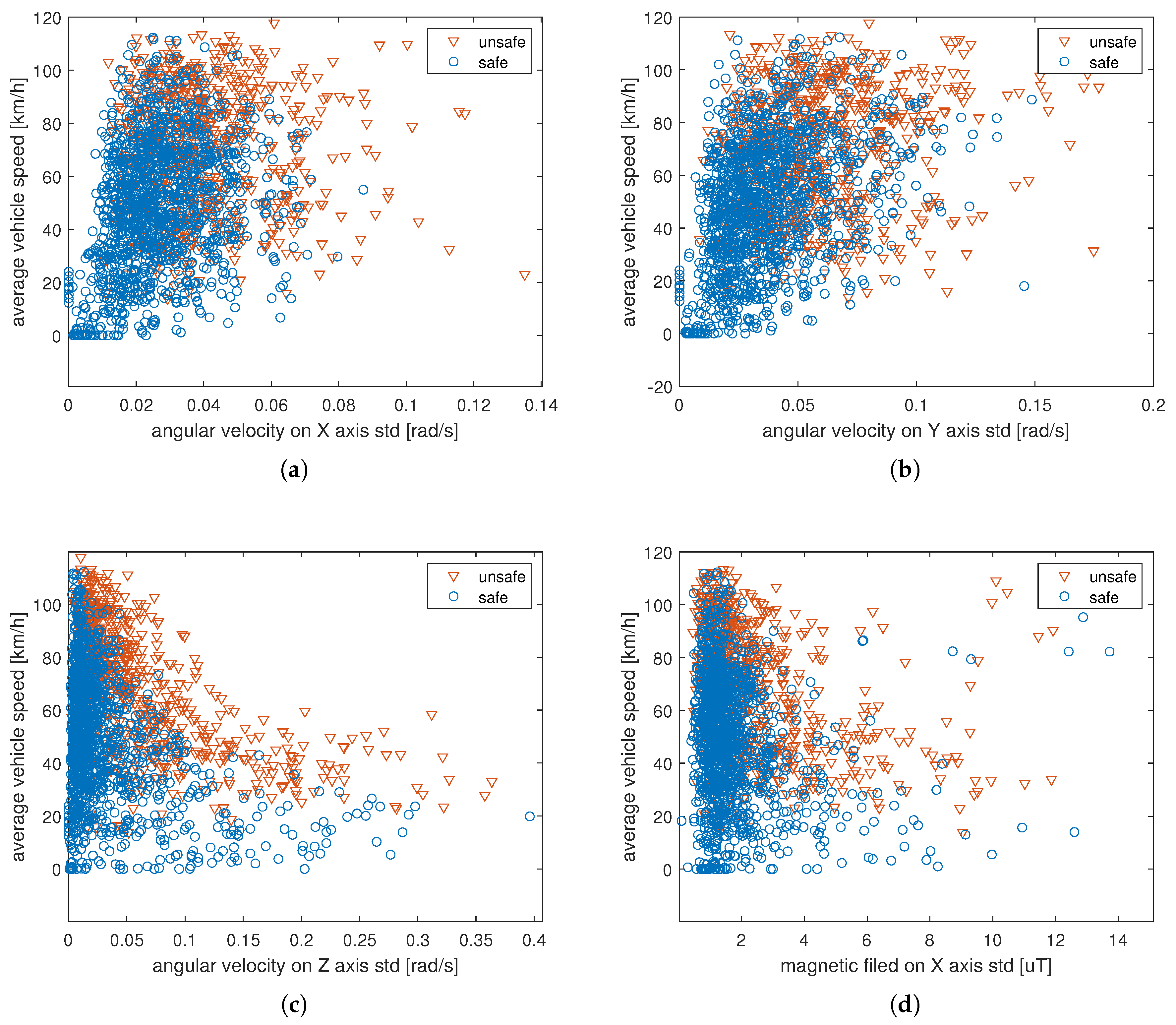
Motion sensors’ features: Motion signals accurately describe the motion of the vehicle which is the result of the driver’s actions on the car controls. In particular, they bring basic information about yaw, pitch, and roll of the vehicle which are fundamental to characterizing the driving behavior. Figure 6a–c shows the standard deviation of the angular velocity versus the vehicle speed, measured by the gyroscope, respectively, around the x, y, and z axes. In all three cases, unsafe behaviors are more frequently associated to the points corresponding at high values of the standard deviation together with high values of the vehicle speed. Since the tree axes directly report pitch, roll, and yaw, it is evident that high variations in these quantities, when traveling at high speed, can easily suggest some unsafe behaviors.

The same trend can be seen in the features calculated starting from the magnetometer signals (Figure 6d–f). In particular, as described in Section 3.2, the x and y axes together can capture information related to pitch, roll, and yaw. Less evident is the separation between safe and unsafe points for the feature calculated over the z axis, as it contains only a singular component of the car pitch.

4.2. Classification Results

Both SVM and neural network classifiers have been trained using the k-fold cross-validation technique with k = 5. To measure the performance of the classifier, the following four metrics have been used:

$$Precision=\frac{TP}{TP+FP}$$

(2)

$$Recall=\frac{TP}{TP+FN}$$

(3)

$$F_{1}score=2·\frac{Precision·Recall}{Precision+Recall}$$

(4)

$$Accuracy=\frac{TP+TN}{TP+TN+FP+FN}$$

(5)

where $TP$ are the true positives, $TN$ the true negatives, $FP$ the false positives, and $FN$ the false negatives.

We also conducted incremental experiments to evaluate the relative importance of the proposed features with respect to the classification performances. In particular, we added, step by step, the groups of features calculated from different sensors in order to highlight their contributions to the classes discrimination. We started training the model with only the in-vehicle sensors’ features, which we believe to be the minimum set; then we added the magnetometer and gyroscope features.

Both training and testing phases have been carried out using Matlab^® on an Asus N56J laptop PC equipped with an Intel^® CORE i7 @ 2.5GHz and 16GB of RAM running Windows 10 Home edition.

SVM results:

Table 1. Confusion matrices and classification performance of the SVM model while trying to distinguish safe and unsafe driver behaviors with different adopted features. Table (a) reports the results obtained with only in-vehicle sensors’ features; Table (b) with in-vehicle sensors and magnetometer features; Table (c) with in-vehicle sensors and gyroscopic features; and Table (d) with all features together.

(a) In-Vehicle				(b) In-Vehicle + Magnetometer
True Class	Predicted Class		Avg	True Class	Predicted Class		Avg
	Safe	Unsafe			Safe	Unsafe
Safe	0.819	0.181	-	Safe	0.868	0.132	-
Unsafe	0.327	0.673	-	Unsafe	0.222	0.778	-
Precision	0.768	0.738	0.753	Precision	0.838	0.817	0.828
Recall	0.819	0.673	0.746	Recall	0.868	0.778	0.823
F1 score	0.792	0.704	0.748	F1 score	0.853	0.797	0.825
Accuracy	0.756	0.756	0.756	Accuracy	0.829	0.829	0.829
(c) In-Vehicle + Gyroscope				(d) In-Vehicle + Magnetometer + Gyroscope
True Class	Predicted Class		Avg	True Class	Predicted Class		Avg
	Safe	Unsafe			Safe	Unsafe
Safe	0.902	0.098	-	Safe	0.910	0.090	-
Unsafe	0.161	0.839	-	Unsafe	0.150	0.850	-
Precision	0.881	0.866	0.873	Precision	0.889	0.877	0.883
Recall	0.902	0.839	0.870	Recall	0.910	0.850	0.880
F1 score	0.891	0.852	0.872	F1 score	0.899	0.863	0.881
Accuracy	0.875	0.875	0.875	Accuracy	0.884	0.884	0.884

reports the confusion matrices and the classification performances of the SVM model when varying the adopted features. The Table 1a shows the results obtained using only the in-vehicle sensors’ features (i.e., speed, engine load, engine rotation speed, and throttle position). In this case, the average classification accuracy reached about 76% and the average precision and recall were about 75%. Notice that the performances of the two classes were appreciably unbalanced, as demonstrated by higher values of the recall and of the F1 score of the “safe” class with respect to the “unsafe” one.

Adding magnetometer features (see Table 1b) increased all average performances, which then became over 82%, by about 7% and also reduced the unbalance about the two classes. For instance, F1 score and recall of the “unsafe” class reached, respectively, 80% and 78%.

Gyroscope features (Table 1c), on the other hand, increased performance metrics even more leading to values close to 87%.

Table 1d reports the results obtained when training the SVM model using all available features. Interestingly, in this configuration, the average classification performances were exceeded by just 1% those obtained when using only in-vehicle sensors plus gyroscopic features as if the signals recorded from the magnetometer did not add useful information compared to those already present in the gyroscope. Moreover, another appreciable variation, obtained in this case appears to be a better balance of the classification performances between the two classes. In the case scenario that consists of using all available features, the execution time of the training phase was 14.925 s, while the prediction of a sample (i.e., of a single vector computed within a 5 s window) was accomplished in 0.357 milliseconds.

Neural network results: The results of the same classification experiments conducted with the feed-forward neural network are reported in

Table 2. Confusion matrices and classification performance of the proposed neural network while trying to distinguish safe and unsafe driver behaviors when varying the adopted features. Table (a) reports the results obtained with only in-vehicle sensors’ features; Table (b) with in-vehicle sensors and gyroscopic features; Table (c) with in-vehicle sensors and magnetometer features; and Table (d) with all features together.

(a) In-Vehicle				(b) In-Vehicle + Magnetometer
True Class	Predicted Class		Avg	True Class	Predicted Class		Avg
	Safe	Unsafe			Safe	Unsafe
Safe	0.802	0.198	-	Safe	0.860	0.140	-
Unsafe	0.236	0.764	-	Unsafe	0.138	0.862	-
Precision	0.827	0.733	0.780	Precision	0.894	0.855	0.874
Recall	0.802	0.764	0.783	Recall	0.890	0.860	0.875
F1 score	0.815	0.748	0.781	F1 score	0.892	0.857	0.875
Accuracy	0.786	0.786	0.786	Accuracy	0.877	0.877	0.877
(c) In-Vehicle + Gyroscope				(d) In-Vehicle + Magnetometer + Gyroscope
True Class	Predicted Class		Avg	True Class	Predicted Class		Avg
	Safe	Unsafe			Safe	Unsafe
Safe	0.909	0.091	-	Safe	0.912	0.088	-
Unsafe	0.132	0.868	-	Unsafe	0.122	0.878	-
Precision	0.898	0.882	0.890	Precision	0.907	0.885	0.896
Recall	0.909	0.868	0.889	Recall	0.912	0.878	0.895
F1 score	0.903	0.875	0.889	F1 score	0.909	0.882	0.896
Accuracy	0.891	0.891	0.891	Accuracy	0.897	0.897	0.897

. With respect to the SVM results, the neural network achieved better performances (measurable in values from about 2% to 5%) in all features configurations, even if essentially it reflects the results obtained by the SVM tool. In fact, also in this case, using only in-vehicle sensors led to a classification performance that sis not exceed the 78% on average, confirming the inadequacy of the extracted features to accurately identify driver behavior. On the other hand, adding a simple gyroscope can strongly compensate for this lack of information, bringing the classification performance up to an average value of about 89%. Finally, using all the available features, the average performance further increased up to about 90%. In this configuration, the training phase lasted 65.491 s while the time to predict a sample was 0.0334 milliseconds.

5. Conclusions

In this work we introduced a methodology based on sensor fusion to improve machine learning recognition of safe and unsafe driving behavior. In particular, we adding to the in-vehicle sensor signals, captured through the OBD-II interface of the vehicle CAN bus, gyroscopic and magnetometer signals from which we computed a set of descriptive features capable to accurately describe the behavior of the driver.

We also proposed to use an objective method in order to label each driving moment as safe or unsafe starting from vehicle motion data according to the work presented by Eboli et al. in 2016 [6]. After data labeling, two different classification tools, namely, an SVM and a feed-forward neural network, were trained and tested over ad hoc gathered data covering more than 200 km traveled by a single driver. The classification results show an average accuracy of about 88% using the SVM classifier and of about 90% using the neural network. Considering that the experiments conducted using only in-vehicle sensors compliant to the OBD-II standard showed an average classification accuracy of about 76%, the increase in performance of more than 12 percentage points, due to the sensor fusion, demonstrates the potential capability of the proposed methodology for identifying driving styles.