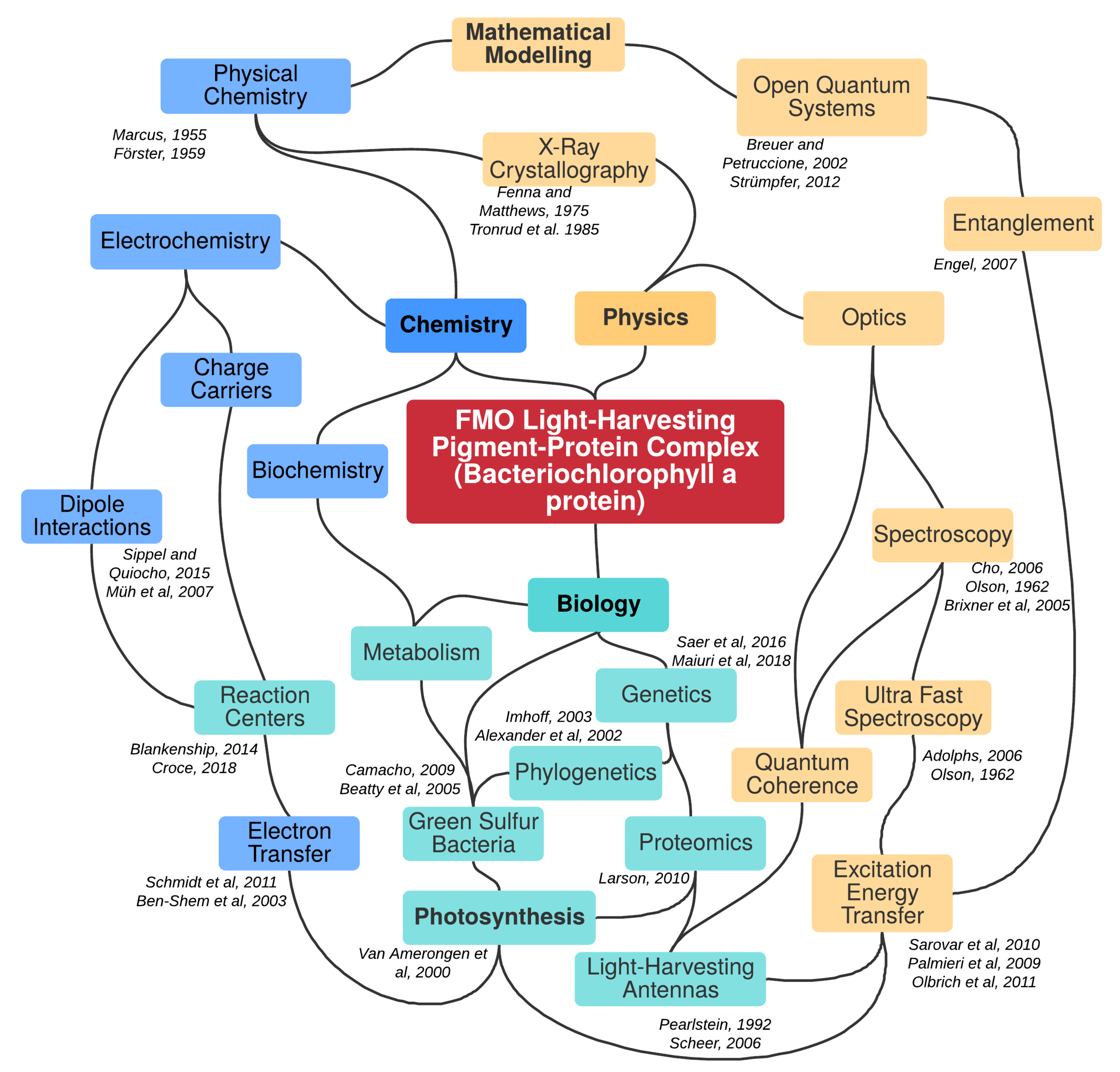
Parametric Mapping of Quantum Regime in Fenna–Matthews–Olson Light-Harvesting Complexes: A Synthetic Review of Models, Methods and Approaches


Abstract
:1. Introduction
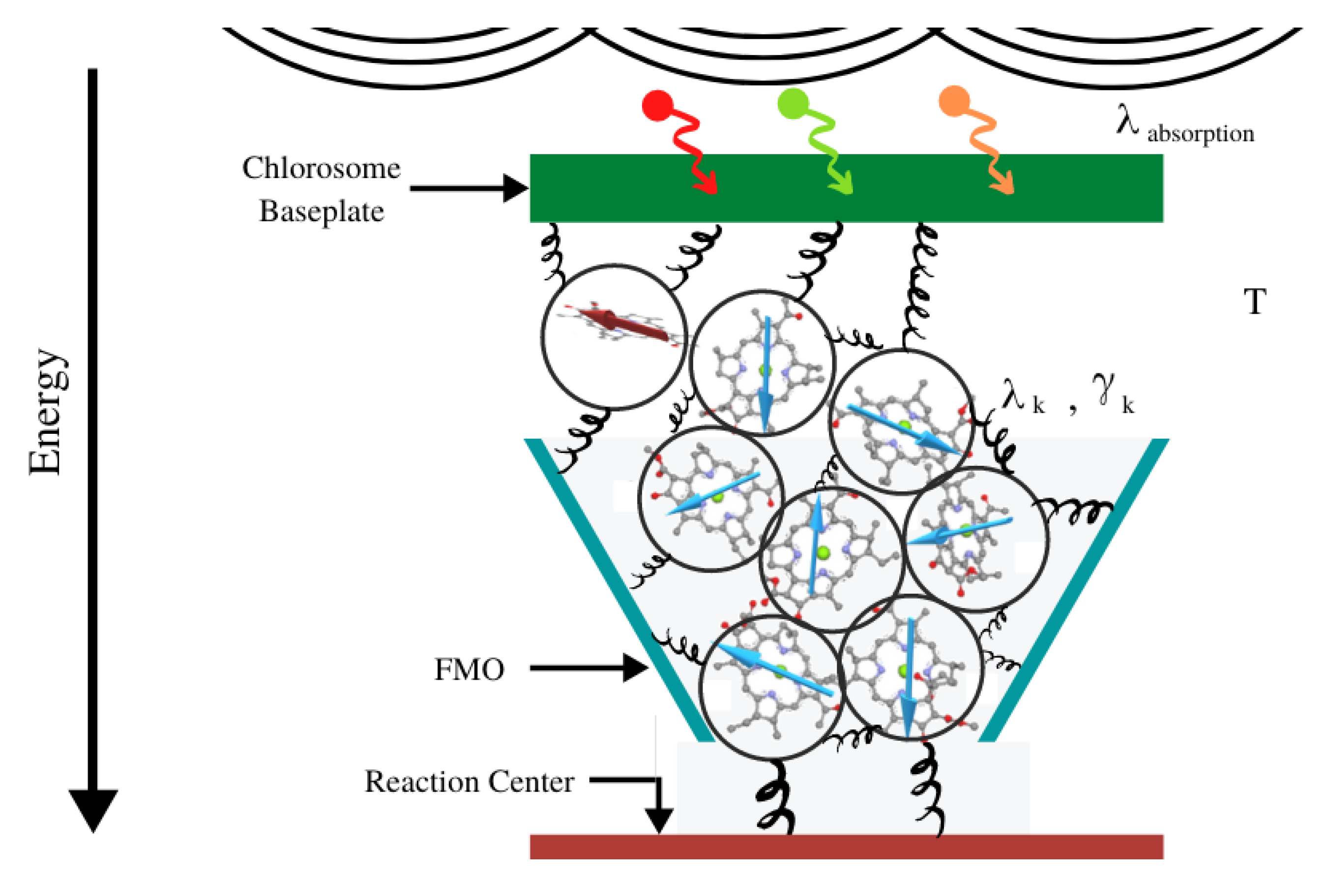
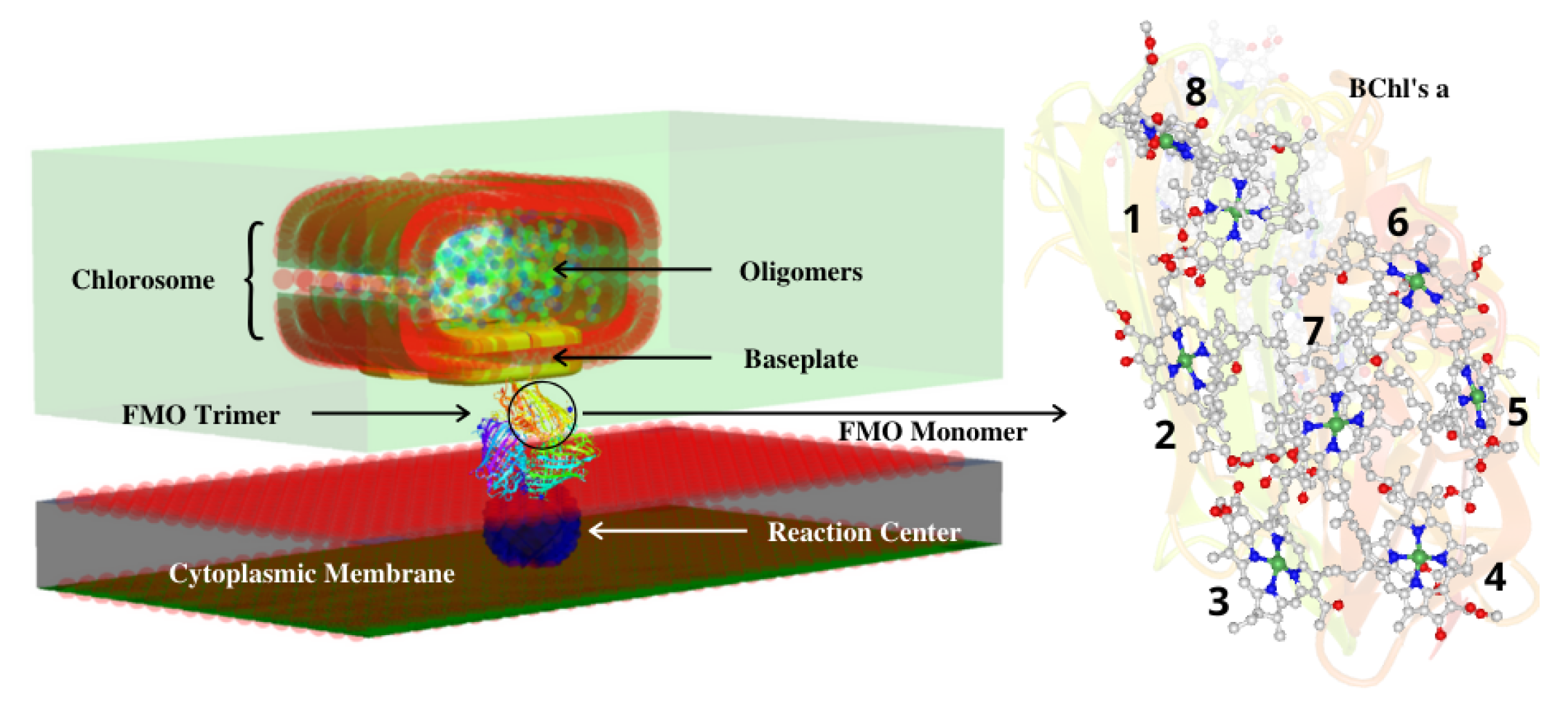
2. Structure of the Fenna–Matthews–Olson Light-Harvesting Complex
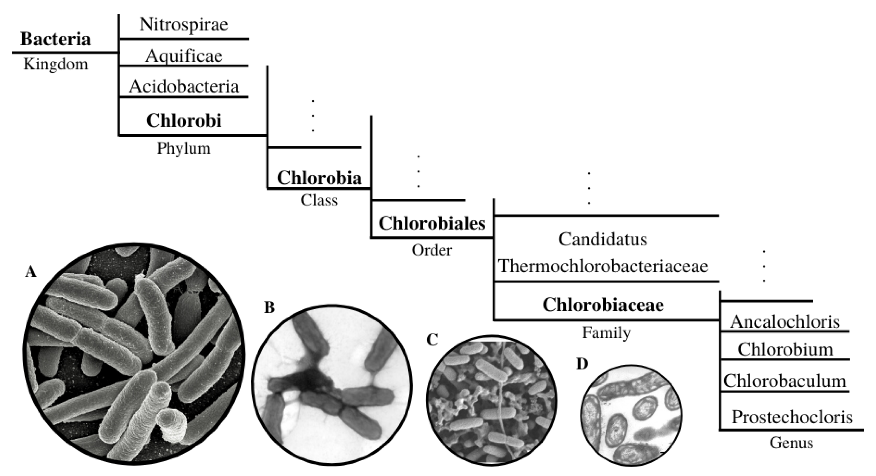
2.1. Green Sulfur Bacteria and the FMO Complex
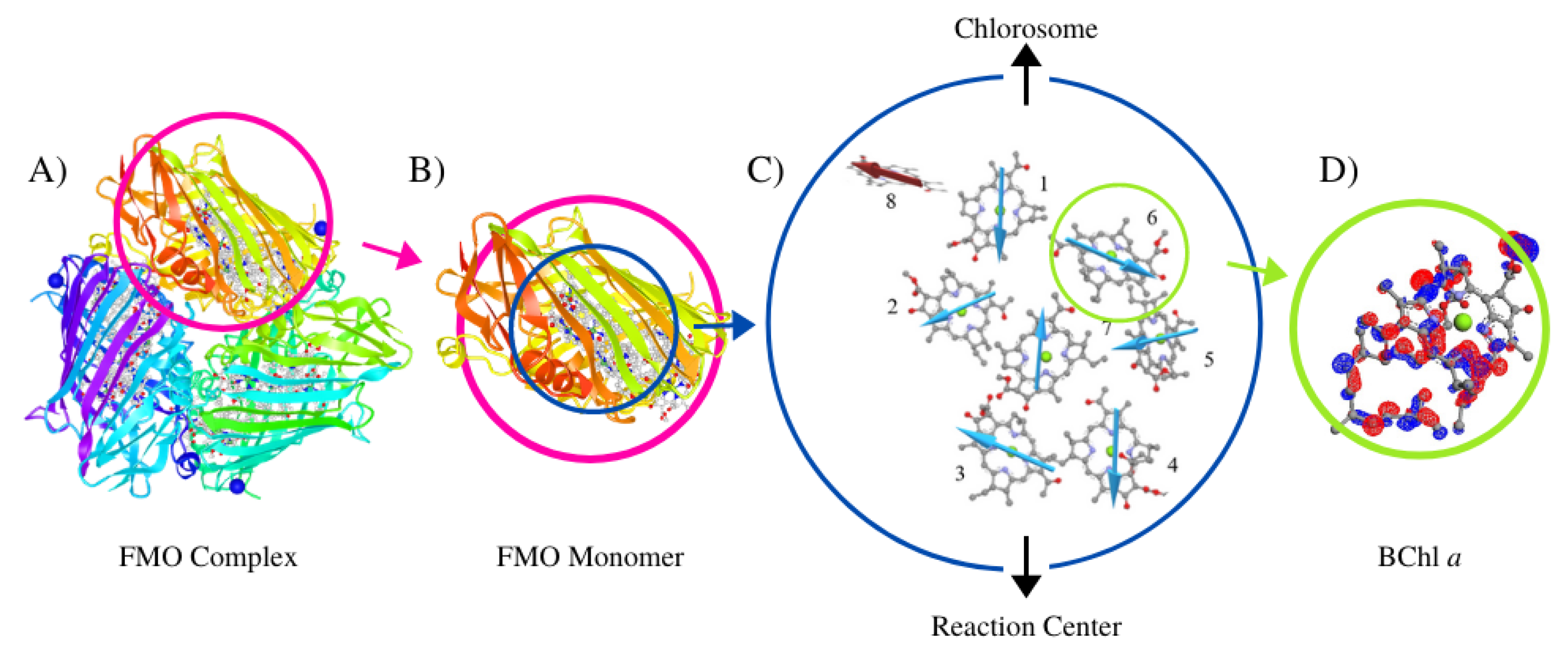
2.2. Structure of the FMO Complex
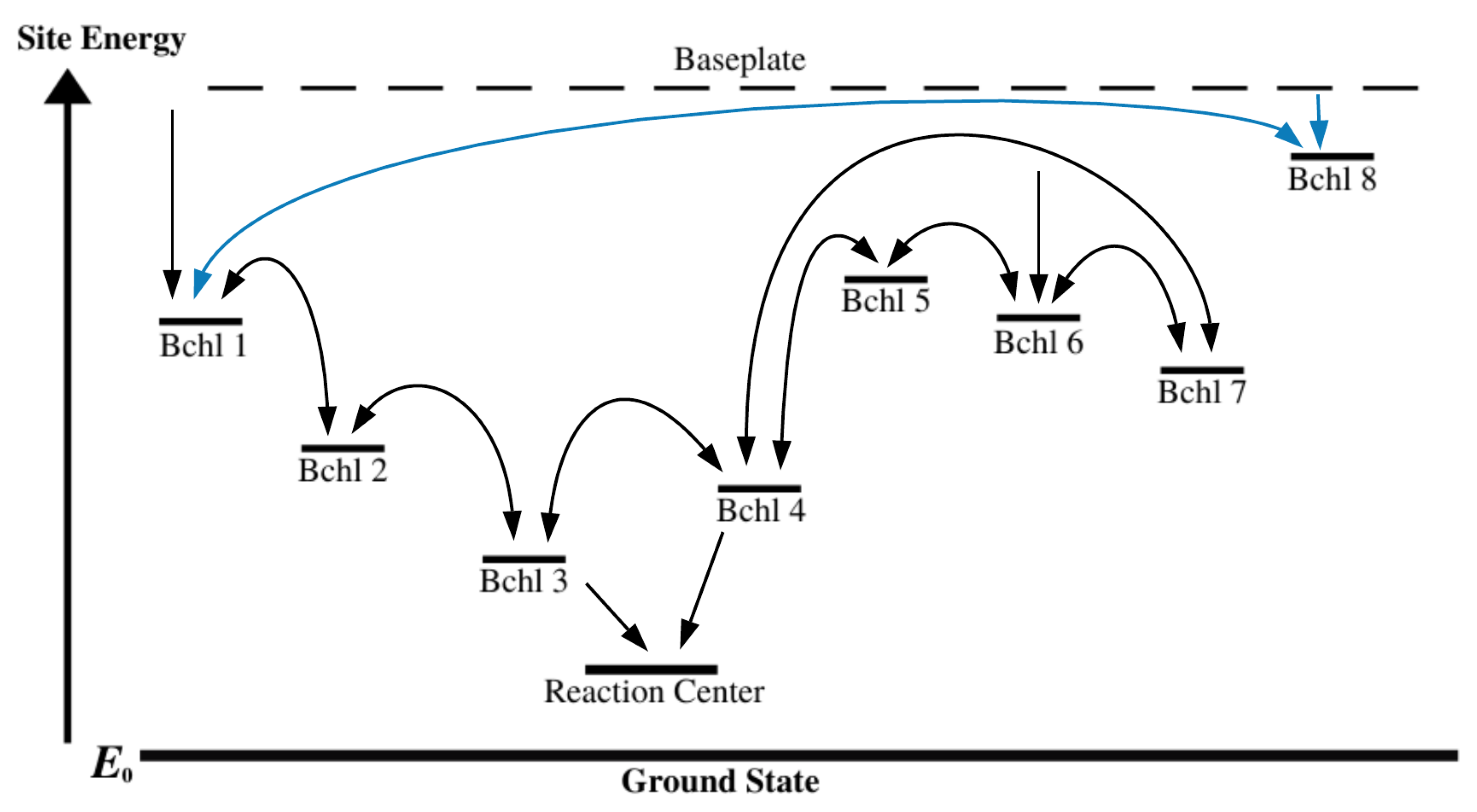
2.3. Interactions within the FMO Complexes and Its Environment
3. Quantum Modelling of FMO Quantum Excitation
3.1. Main Dipole Interactions among BChls
3.2. Construction of the Entire Hamiltonian to Model FMO Complex
3.3. LHCs As Open Quantum Systems
3.3.1. Lindblad Approach to FMO Complexes Modelling
3.3.2. Redfield Approach to FMO Complexes Modelling
3.3.3. HEOM Method Approach in FMO Complexes Models
3.4. Superoperator Version of Master Equations
4. Numerical Solving of HEOM Models and Analysis of Physical Measures to Feature Parametrically the Quantum Regime in the FMO Complex
4.1. Methods, Extent of Analysis, and Source Data
4.1.1. Computer Resources in the Modelling
4.1.2. Ranges and Extent of the Parametric Analysis
4.1.3. Data Source Methodology
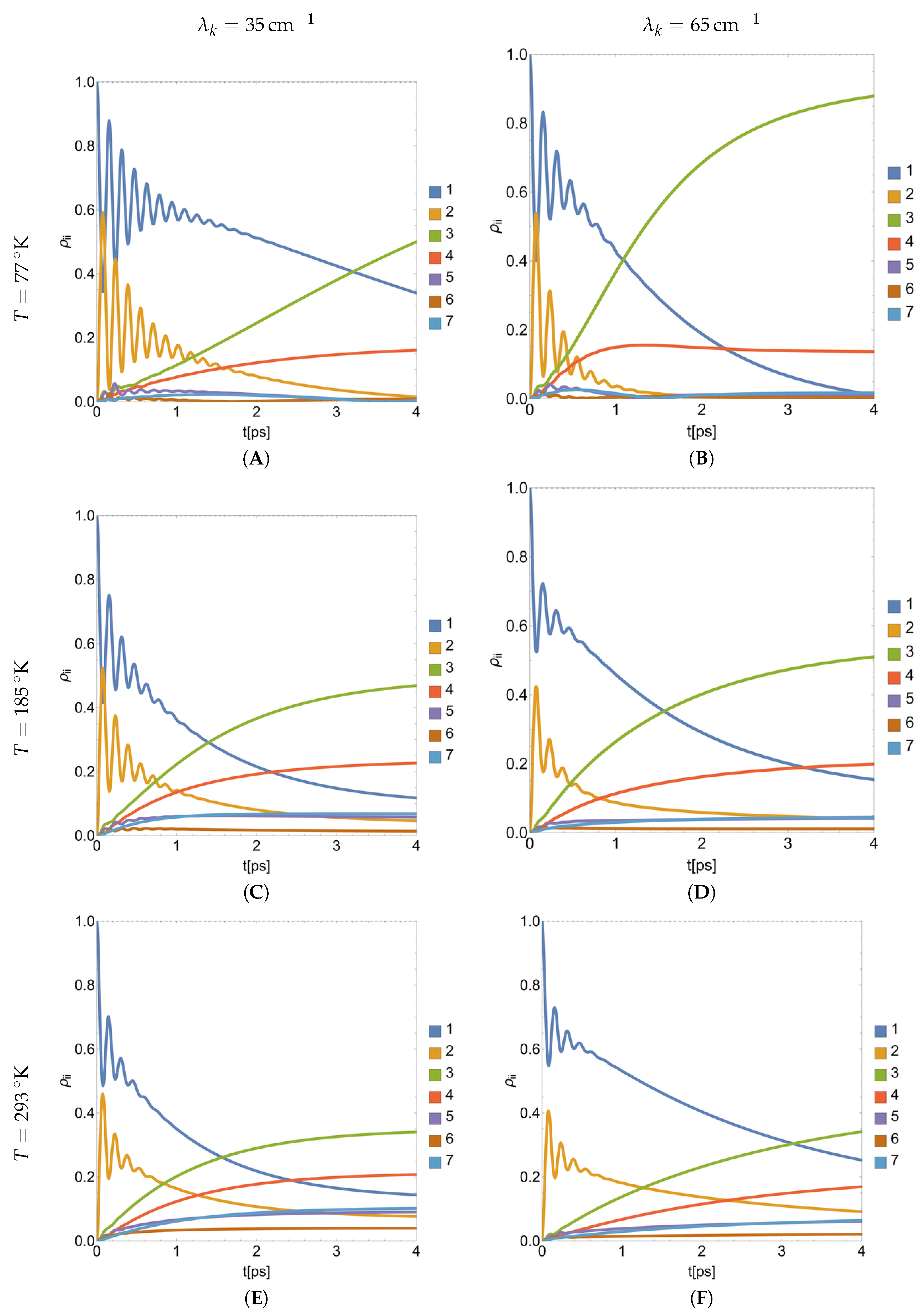
4.1.4. Source Data Generated from Computer Simulations
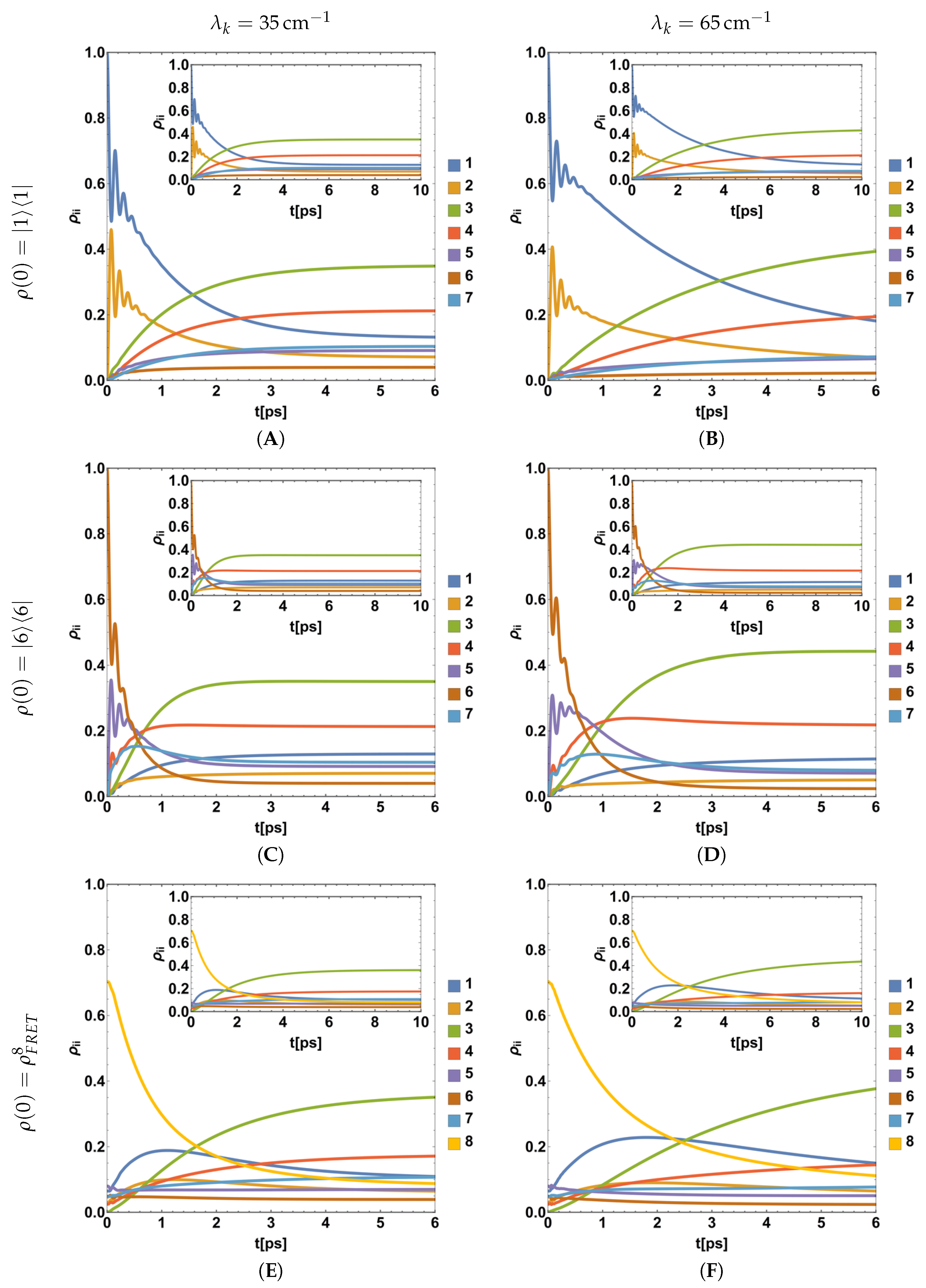
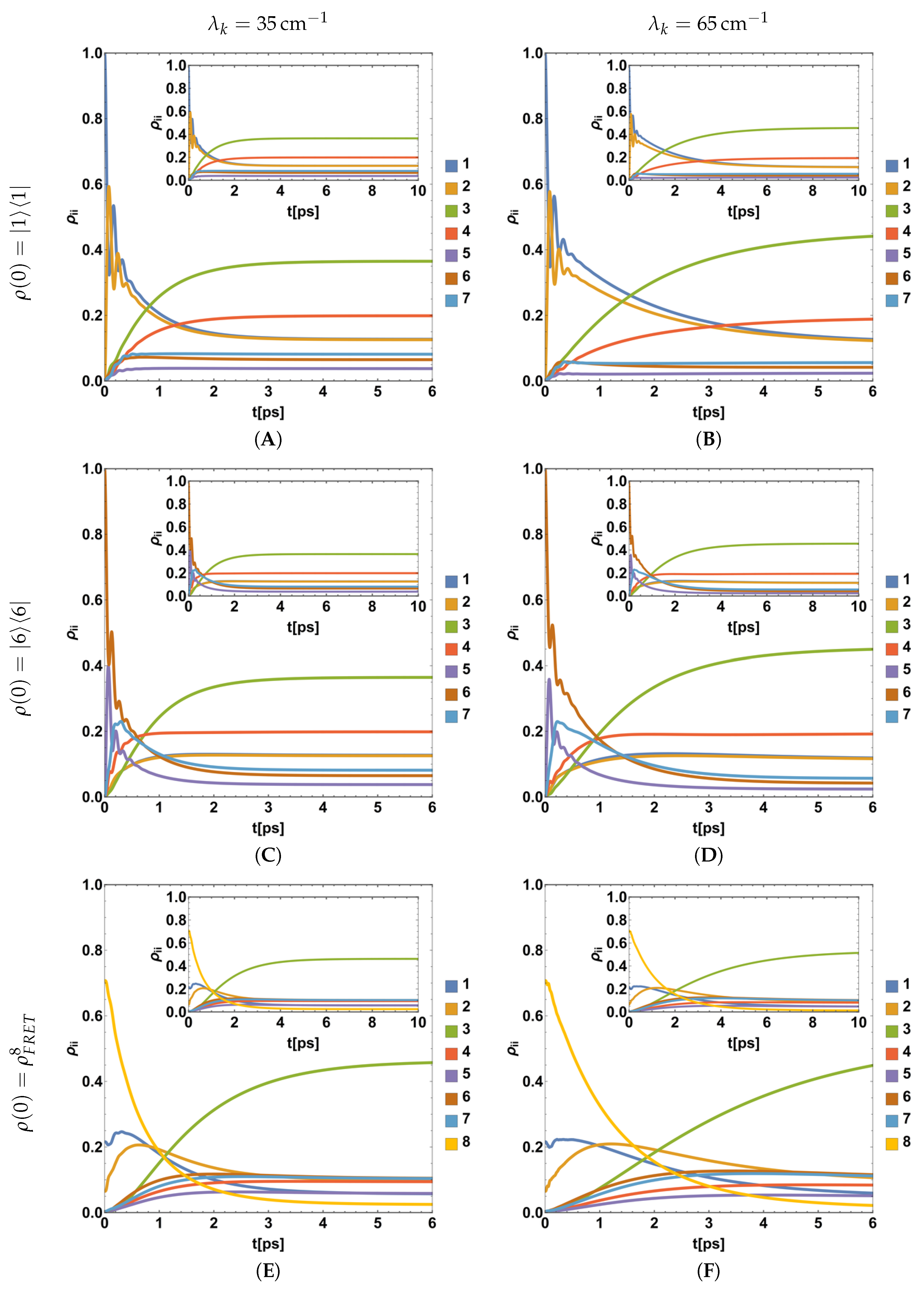
4.2. Parametric Dynamics of Populations during the BChls Excitation
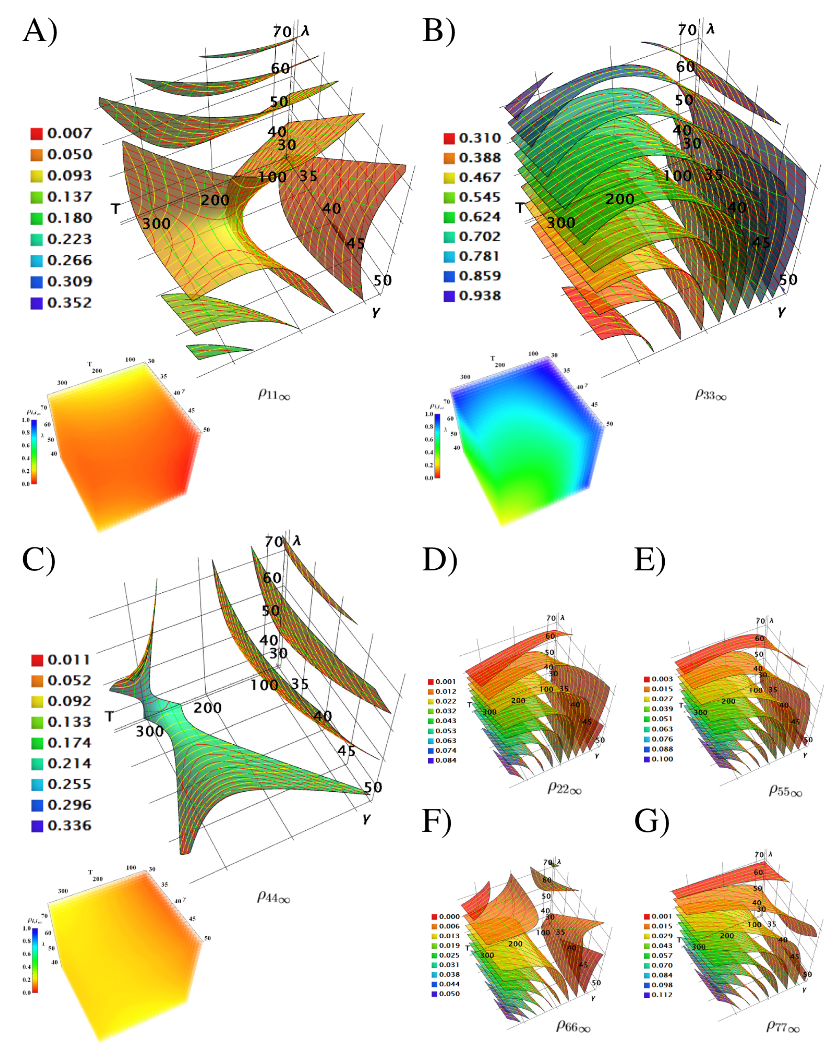
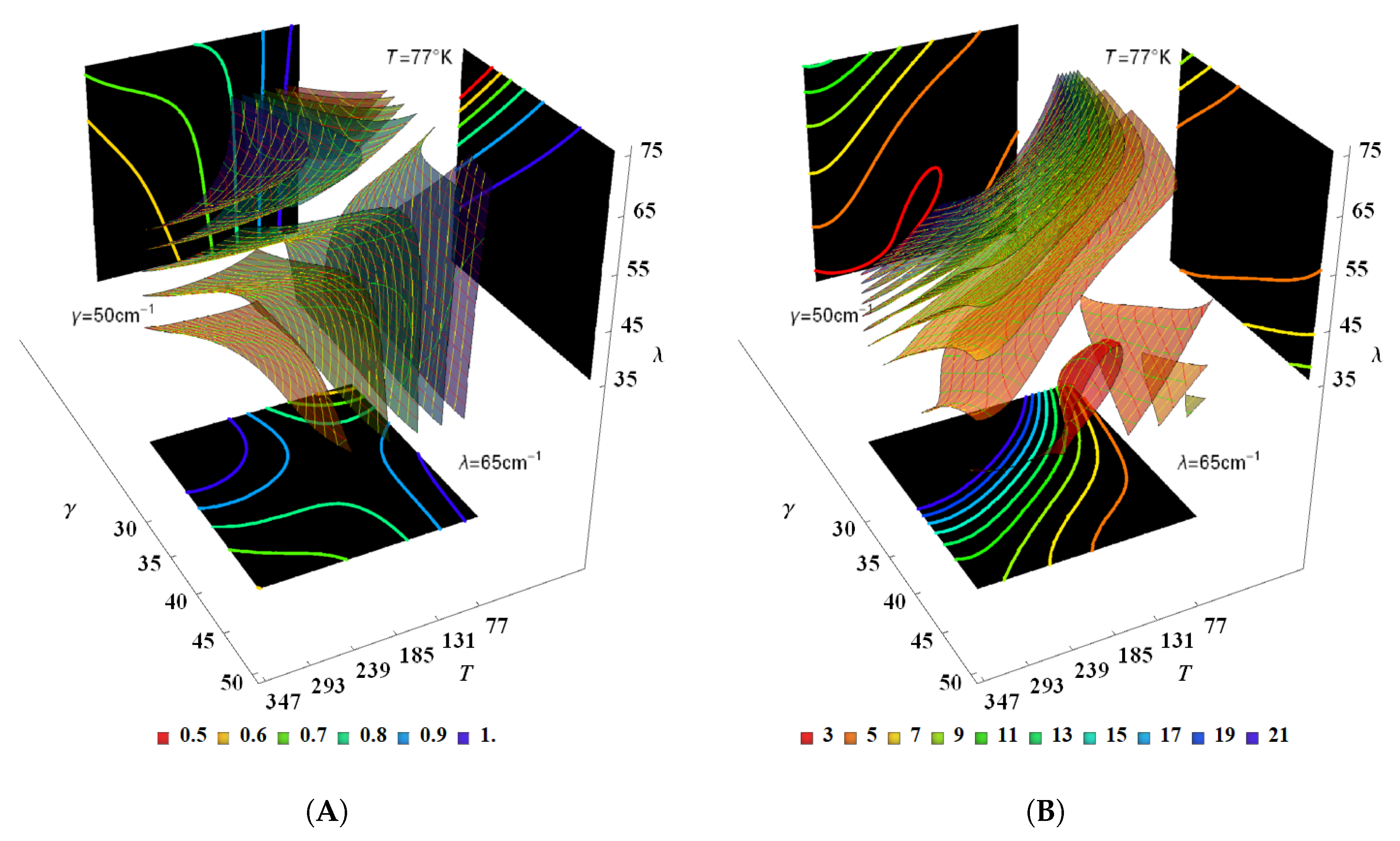
4.3. Quantum Populations Reached in the Equilibrium Depending of and
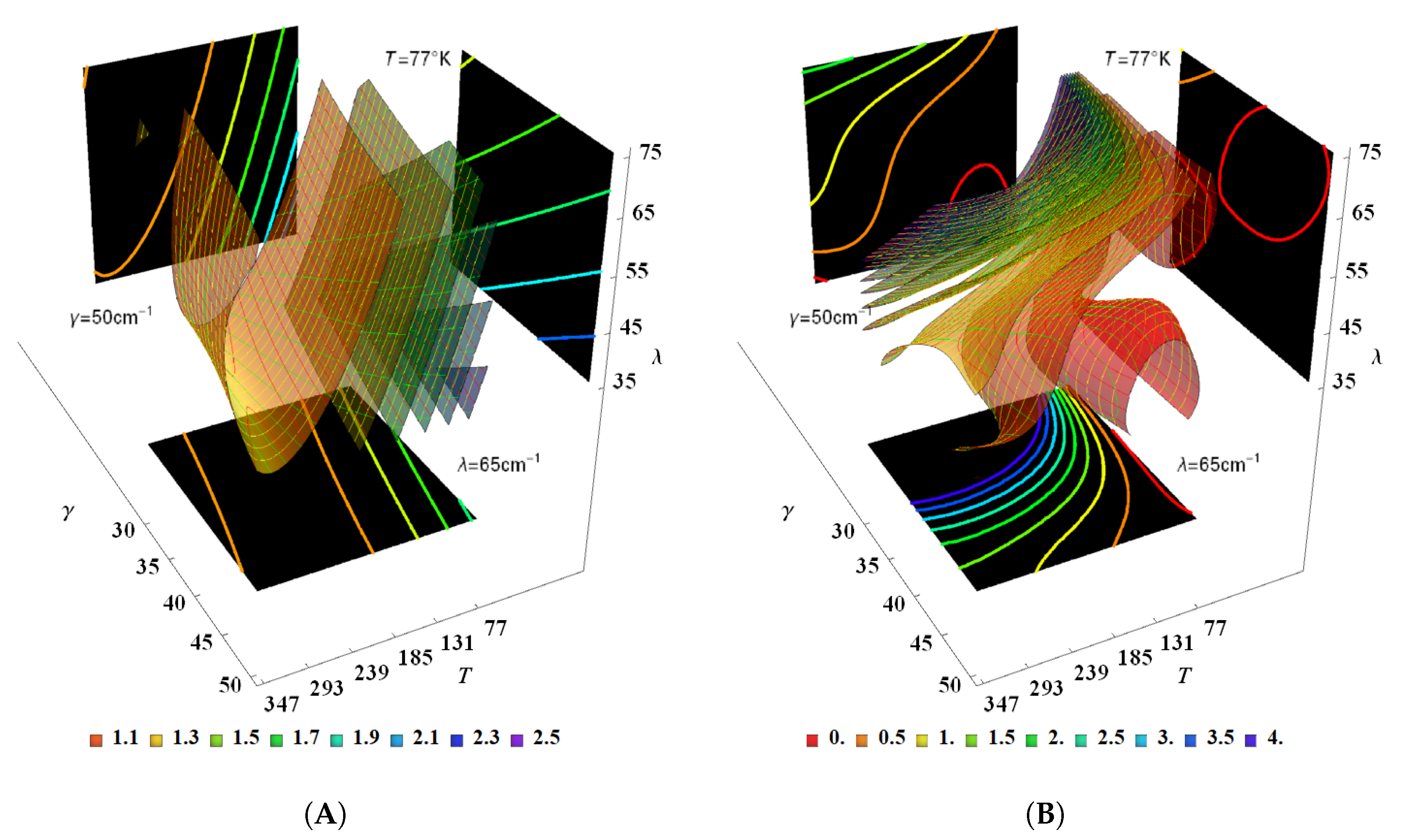
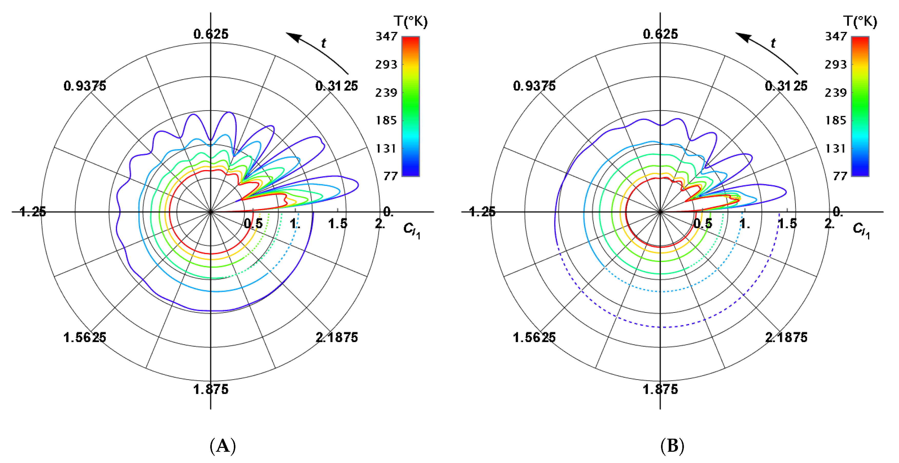
4.4. Coherence Depending of and
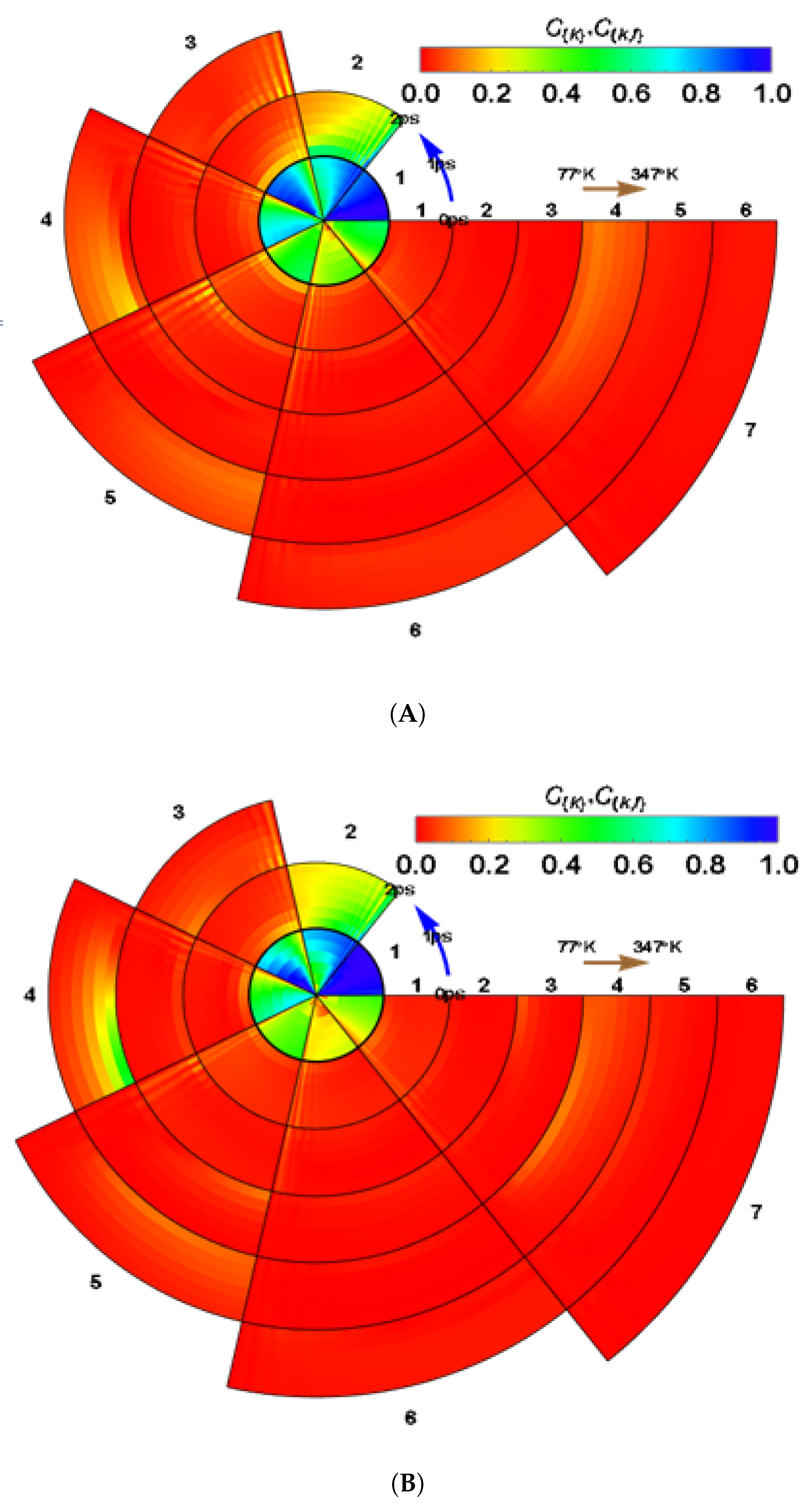
4.5. Entanglement Generation Depending of and
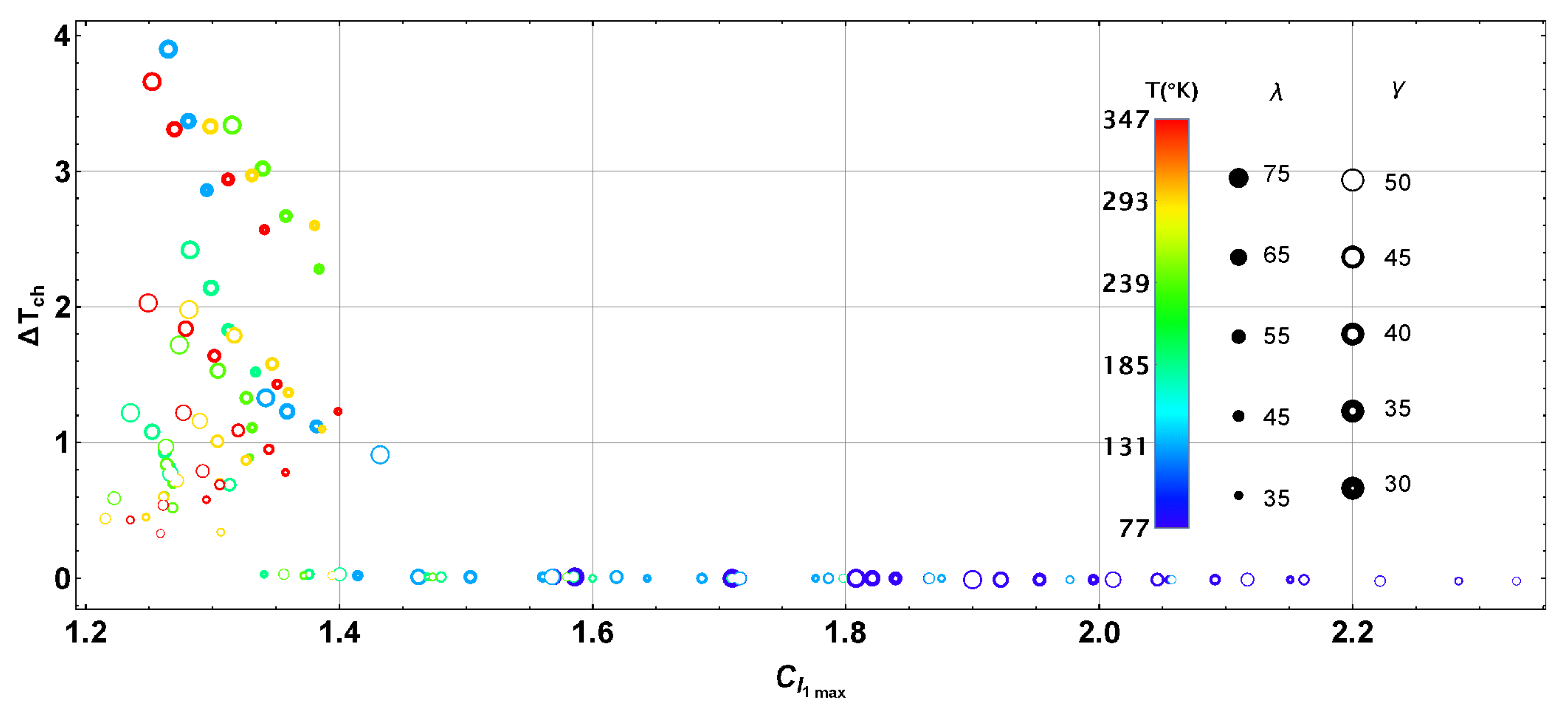
4.6. Efficiency Depending of and
5. Characterization of Genetic Differences in the FMO Complexes with other Species and Strains
5.1. Alternative and Extended Studies on FMO for other Species and Strains
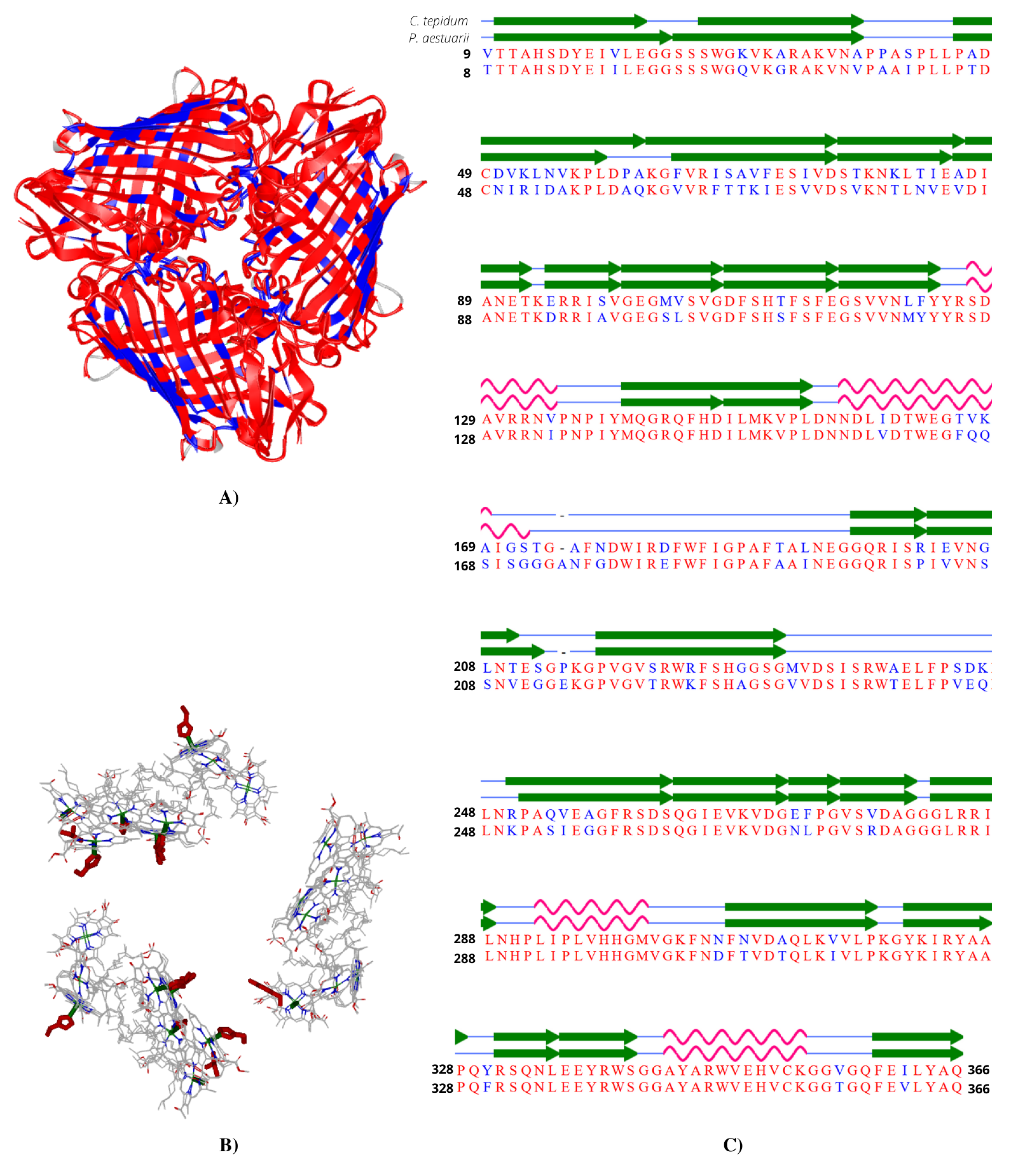
5.2. Comparative Analysis between Chlorobaculum tepidum and Prosthecochloris aestuarii
5.3. Genetic and Structural Differences between Species and Strains and Their Manipulation
6. Conclusions
Author Contributions
Funding
Acknowledgments
Conflicts of Interest
Abbreviations
| FMO | Fenna-Matthews-Olson |
| LHC, LHCs | Light-Harvesting Complex, Light-Harvesting Complexes |
| BChl, BChls | Bacteriochlorophyll, Bacteriochlorophylls |
| HEOM | Hierarchical Equations of Motion |
| RC | Reaction Center |
| GBS | Green Sulfur Bacteria |
| EET | Excitation Energy Transfer |
| FRET | Förster Resonance Energy Transfer |
Appendix A. Dipole–Dipole Hamiltonians for N = 7 and N = 8 BChls
Appendix B. Linblad Equation Derivation in Brief
Appendix C. Redfield Equation Derivation in Brief
Appendix D. Translating Master Equations into Matrix Differential Linear Equations
References
- am Busch, M.S.; Müh, F.; Madjet, M.E.A.; Renger, T. The Eighth Bacteriochlorophyll Completes the Excitation Energy Funnel in the FMO Protein. J. Phys. Chem. Lett. 2011, 2, 93–98. [Google Scholar] [CrossRef]
- Croce, R.; van Grondelle, R.; van Amorengen, H.; van Stokkum, I. Light Harvesting in Photosynthesis; Taylor & Francis Group: Boca Raton, FL, USA, 2018; pp. 247–378. [Google Scholar]
- Leibl, W.; Trissl, H.W. Relationship between the fraction of closed photosynthetic reaction centers and the amplitude of the photovoltage from light-gradient experiments. Biochim. Biophys. Acta 1990, 1015, 304–312. [Google Scholar] [CrossRef]
- Blankenship, R.E. Molecular Mechanisms of Photosynthesis; Wiley Blackwell: St. Louis, MO, USA, 2014; pp. 41–82. [Google Scholar]
- Marcus, R.; Sutin, N. Electron transfer in chemistry and biology. Biochim. Biophys. Acta 1985, 811, 265–322. [Google Scholar] [CrossRef]
- Förster, T. Transfer Mechanisms of Electronic Excitation. Discuss. Faraday Soc. 1959, 27, 7–17. [Google Scholar] [CrossRef]
- Fenna, R.E.; Matthews, B.W. Chlorophyll arrangement in a bacteriochlorophyll protein from Chlorobium limicola. Nature 1975, 258, 573–577. [Google Scholar] [CrossRef]
- Fenna, R.E.; Matthews, B.W.; Olson, J.M. Structure of a Bacteriochlorophyll a-Protein from the Green Photosynthetic Bacterium Prosthecochloris aestuarii. J. Mol. Biol. 1978, 131, 259–285. [Google Scholar]
- Ravi, S.K.; Swainsbury, D.J.K.; Singh, V.K.; Ngeow, Y.K.; Jones, M.R.; Tan, S.C. A Mechanoresponsive Phase-Changing Electrolyte Enables Fabrication of High-Output Solid-State Photobiolectrochemical Devices from Pigment-Protein Multilayers. Adv. Mater. 2017, 1704073, 1–8. [Google Scholar]
- Vattay, G.; Kauffman, S. Evolutionary Design in Biological Quantum Computing. arXiv 2013, arXiv:1311.4688v1. [Google Scholar]
- Ben-Shem, A.; Frolow, F.; Nelson, N. Evolution of photosystem I—From symmetry through pseudosymmetry to asymmetry. FEBS Lett. 2004, 564, 274–280. [Google Scholar] [CrossRef] [Green Version]
- Tronrud, D.E.; Wen, J.; Gay, L.; Blankenship, R.E. The structural basis for the difference in absorbance spectra for the FMO antenna protein from various green sulfur bacteria. Photosyn. Res. 2009, 100, 79–87. [Google Scholar] [CrossRef] [PubMed]
- Adolphs, J.; Renger, T. How proteins trigger excitation energy transfer in the FMO complex of green sulfur bacteria. Biophys. J. 2006, 91, 2778–2797. [Google Scholar] [CrossRef] [Green Version]
- Müh, F.; Madjet, M.E.A.; Adolphs, J.; Abdurahman, A.; Rabenstein, B.; Ishikita, H.; Knapp, E.W.; Renger, T. α-Helices direct excitation energy flow in the Fenna-Matthews-Olson protein. Proc. Natl. Acad. Sci. USA 2007, 104, 16862–16867. [Google Scholar] [CrossRef] [Green Version]
- Camacho, A. Sulfur Bacteria. In Encyclopedia of Inland Waters; Elsevier; University of Valencia: Burjassot, Spain, 2009; pp. 261–278. [Google Scholar]
- Beatty, J.T.; Overmann, J.; Lince, M.T.; Manske, A.K.; Lang, A.S.; Blankenship, R.E.; Dover, C.L.V.; Martinson, T.A.; Plumley, F.G. An obligately photosynthetic bacterial anaerobe from a deep-sea hydrothermal vent. Proc. Natl. Acad. Sci. USA 2005, 102, 9306–9310. [Google Scholar] [CrossRef] [Green Version]
- Blankenship, R.E.; Olson, J.M.; Miller, M. Anoxygenic Photosynthetic Bacteria—Antenna Complexes from Green Photosynthetic Bacteria; Kluwer Academic Publishers: Dordrecht, The Netherlands, 1995; pp. 399–435. [Google Scholar]
- Alexander, B.; Andersen, J.H.; Cox, R.P.; Imhoff, J.F. Phylogeny of green sulfur bacteria on the basis of gene sequences of 16S rRNA and of the Fenna-Matthews-Olson protein. Arch. Microbiol. 2002, 178, 131–140. [Google Scholar] [CrossRef]
- Saer, R.G.; Satnytskyi, V.; Magdaong, N.C.; Goodson, C.; Savikhin, S.; Blankenship, R.E. Probing the excitonic landscape of the Clorobaculum tepidum Fenna-Matthews-Olson (FMO) complex: A mutagenesis approach. Biochim. Biophys. Acta 2017, 1858, 288–296. [Google Scholar] [CrossRef]
- Maiuri, M.; Ostroumov, E.E.; Saer, R.G.; Blankenship, R.E.; Scholes, G.D. Coherent wavepackets in the Fenna-Matthews-Olson complex are robust to excitonic-structure perturbations caused by mutagenesis. Nat. Chem. 2018, 10, 177–183. [Google Scholar] [CrossRef]
- van Amerongen, H.; Valkunas, L.; van Grondelle, R. Photosynthetic Excitons; World Scientific: Danvers, MA, USA, 2000; pp. 449–478. [Google Scholar]
- Engel, G.S.; Calhoun, T.R.; Read, E.L.; Ahn, T.K.; Mančal, T.; Cheng, Y.C.; Blankenship, R.E.; Fleming, G.R. Evidence for wavelike energy transfer through quantum coherence in photosynthetic systems. Nature 2007, 446, 782–786. [Google Scholar] [CrossRef]
- Panitchayangkoon, G.; Hayes, D.; Fransted, K.A.; Caram, J.R.; Harel, E.; Wen, J.; Blankenship, R.E.; Engel, G.S. Long-lived quantum coherence in photosynthetic complexes at physiological temperature. Proc. Natl. Acad. Sci. USA 2010, 107, 12766–12770. [Google Scholar] [CrossRef] [Green Version]
- Savikhin, S.; Buck, D.R.; Struve, W.S. Oscillating anisotropies in a bacteriochlorophyll protein: Evidence for quantum beating between exciton levels. Chem. Phys. 1997, 223, 303–312. [Google Scholar] [CrossRef]
- Wilkins, D.M.; Dattani, N.S. Why Quantum Coherence Is Not Important in the Fenna–Matthews–Olsen Complex. J. Chem. Theory Comput. 2015, 11, 3411–3419. [Google Scholar] [CrossRef] [Green Version]
- Fassioli, F.; Dinshaw, R.; Arpin, P.C.; Scholes, G.D. Photosynthetic light harvesting: Excitons and coherence. J. R. Soc. Interface 2014, 11, 20130901. [Google Scholar] [CrossRef] [PubMed]
- Leon-Montiel, R.D.J.; Kassal, I.; Torres, J.P. The Importance of Excitation and Trapping Conditions in Photosynthetic Environment-assisted Energy Transport. J. Phys. Chem. B 2014, 118, 10588–10594. [Google Scholar]
- Rebentrost, P.; Mohseni, M.; Kassal, I.; Lloyd, S.; Aspuru-Guzik, A. Environment-assisted quantum transport. New J. Phys. 2009, 11, 033003. [Google Scholar] [CrossRef]
- Caruso, F.; Chin, A.W.; Datta, A.; Huelga, S.F.; Plenio, M.B. Highly efficient energy excitation transfer in light-harvesting complexes: The fundamental role of noise-assisted transport. J. Chem. Phys. 2009, 131, 105106. [Google Scholar] [CrossRef] [Green Version]
- Mohseni, M.; Rebentrost, P.; Lloyd, S.; Aspuru-Guzik, A. Environment-assisted quantum walks in photosynthetic energy transfer. J. Chem. Phys. 2008, 129, 174106. [Google Scholar] [CrossRef] [PubMed] [Green Version]
- Plenio, M.B.; Huelga, S.F. Dephasing assisted transport: Quantum networks and biomolecules. arXiv 2008, arXiv:0807.4902v1. [Google Scholar] [CrossRef]
- Sahoo, P.K.; Benjamin, C. Testing quantum speedups in exciton transport through a photosynthetic complex using quantum stochastic walks. arXiv 2020, arXiv:2004.02938. [Google Scholar]
- Olson, J.M.; Romano, C.A. A New Chlorophyll from Green Bacteria. Biochim. Biophys. Acta 1962, 59, 726–728. [Google Scholar] [CrossRef] [Green Version]
- Wen, J.; Zhang, H.; Gross, M.L.; Blankenship, R.E. Native Electrospray Mass Spectrometry Reveals the nature and Stoichiometry of Pigments in the FMO Photosynthesis Antenna Protein. Biochemistry 2011, 50, 3502–3511. [Google Scholar] [CrossRef] [Green Version]
- Hayes, D.; Engel, G.S. Extracting the Excitonic Hamiltonian of the Fenna-Matthews-Olson Complex Using Three-Dimensional Third-Order Electronic Spectroscopy. Biophys. J. 2011, 100, 2043–2052. [Google Scholar] [CrossRef] [Green Version]
- Palmieri, B.; Abramavicius, D.; Mukamel, S. Lindblad equations for strongly coupled populations and coherences in photosynthetic complexes. J. Chem. Phys. 2009, 130, 204512. [Google Scholar] [CrossRef] [PubMed] [Green Version]
- Kell, A.; Blankenship, R.E.; Jankowiak, R.J. Effect of Spectral Density Shapes on the Excitonic Structure and Dynamics of the Fenna-Matthews-Olson Trimer From Chlorobaculum Tepidum. J. Phys. Chem. 2016, 120, 6146–6154. [Google Scholar] [CrossRef] [PubMed]
- Kreisbeck, C.; Kramer, T.; Rodriguez, M.; Hein, B. High-Performance Solution of Hierarchical Equations of Motion for Studying Energy Transfer in Light-Harvesting Complexes. J. Chem. Theory Comput. 2011, 7, 2166–2174. [Google Scholar] [CrossRef] [PubMed] [Green Version]
- Gilmore, J.; McKenzie, R.H. Quantum Dynamics of Electronic Excitations in Biomolecular Chromophores: Role of the Protein Environment and Solvent. J. Phys. Chem. A 2008, 112, 2162–2176. [Google Scholar] [CrossRef] [Green Version]
- Jackson, J.D. Electrodynamics, Classical. In Digital Encyclopedia of Applied Physics; Wiley-VCH Verlag GmbH and Co. KGaA: New York, NY, USA, 1999; pp. 259–294. [Google Scholar]
- Singh, D.; Dasgupta, S. Role of Initial Coherence in Excitation Energy Transfer in Fenna-Matthews-Olson Complex. arXiv 2017, arXiv:1708.00920v2. [Google Scholar]
- Weidemüller, M. There can be only one. Nat. Phys. 2009, 5, 91–92. [Google Scholar] [CrossRef]
- Sarovar, M.; Ishizaki, A.; Fleming, G.; Whaley, K. Quantum entanglement in photosynthetic light-harvesting complexes. Nat. Phys. 2010, 6, 462–467. [Google Scholar] [CrossRef]
- Brixner, T.; Stenger, J.; Vaswani, H.M.; Cho, M.; Blankenship, R.E.; Fleming, G. Two-dimensional spectroscopy of electronic couplings in photosynthesis. Nature 2005, 434, 625–628. [Google Scholar] [CrossRef] [PubMed]
- Olbrich, C.; Jansen, T.L.C.; Liebers, J.; Aghtar, M.; Strümpfer, J.; Schulten, K.; Knoester, J.; Kleinekathöfer, U. From Atomistic Modeling to Excitation Transfer and Two-Dimensional Spectra of the FMO Light-Harvesting Complex. J. Phys. Chem. B 2011, 115, 8609–8621. [Google Scholar] [CrossRef] [Green Version]
- Shabani, A.; Mohseni, M.; Rabitz, H.; Lloyd, S. Optimal and Robust energy transfer in light-harvesting complexes Efficient simulation of excitonic dynamics in the non-perturbative and non-markovian regimes. arXiv 2011, arXiv:1103.3823v2. [Google Scholar]
- Jesenko, S.; Žnidarič, M. Optimal number of pigments in photosynthetic complexes. New J. Phys. 2012, 14, 093017. [Google Scholar] [CrossRef]
- Jeske, J.; Ing, D.J.; Plenio, M.B.; Huelga, S.F.; Cole, J.H. Bloch-Redfield equations for modeling light-harvesting complexes. J. Chem. Phys. 2015, 142, 064104. [Google Scholar] [CrossRef] [PubMed] [Green Version]
- Tanimura, Y.; Kubo, R. Time Evolution of a Quantum System in Contact with a Nearly Gaussian-Markoffian Noise Bath. J. Phys. Soc. Jpn. 1989, 58, 101–114. [Google Scholar] [CrossRef]
- Breuer, H.P.; Laine, E.M.; Piilo, J.; Vacchini, B. Colloquium: Non-Markovian dynamics in open quantum systems. Rev. Mod. Phys. 2016, 88, 021002. [Google Scholar] [CrossRef] [Green Version]
- Bengtson, C.; Stenrup, M.; Sjöqvist, E. Quantum nonlocality in the excitation energy transfer in the Fenna-Matthews-Olson complex. arXiv 2018, arXiv:1502.07842v3. [Google Scholar] [CrossRef] [Green Version]
- González-Soria, B.; Delgado, F.; Anaya-Morales, A. Predicting entanglement and coherent times in FMO complex using the HEOM method. arXiv 2020, arXiv:2008.07580. [Google Scholar]
- Fleming, G.R.; Cho, M. Chromophore-Solvent Dynamics. Annu. Rev. Phys. Chem. 1996, 47, 109–134. [Google Scholar] [CrossRef] [Green Version]
- Cho, M.; Vaswani, H.M.; Brixner, T.; Stenger, J.; Fleming, G.R. Exciton Analysis in 2D Electronic Spectroscopy. J. Phys. Chem. B 2005, 109, 10542–10556. [Google Scholar] [CrossRef]
- Mohseni, M.; Shabani, A.; Lloyd, S.; Rabitz, H. Energy-scales convergence for optimal and robust quantum transport in photosynthetic complexes. J. Chem. Phys. 2014, 140, 035102. [Google Scholar] [CrossRef] [Green Version]
- Kramer, T.; Rodriguez, M. Two-dimensional electronic spectra of the photosynthetic apparatus of green sulfur bacteria. Sci. Rep. 2017, 7, 45245. [Google Scholar] [CrossRef] [Green Version]
- Hauska, G.; Schoedl, T.; Remigy, H.; Tsiotis, G. The reaction center of green sulfur bacteria. Biochim. Biophys. Acta 2001, 1507, 260–277. [Google Scholar] [CrossRef] [Green Version]
- González-Soria, B.; Delgado, F. Quantum Entanglement in Fenna-Matthews-Olson Photosynthetic Light-Harvesting Complexes: A short Review of Analysis Methods. J. Phys. Conf. Ser. 2020, 1540, 012026. [Google Scholar] [CrossRef]
- Baumgratz, T.; Cramer, M.; Plenio, M.B. Quantifying Coherence. Phys. Rev. Lett. 2014, 113, 140401. [Google Scholar] [CrossRef] [PubMed] [Green Version]
- Horn, R.A.; Johnson, C.R. Matrix Analysis; Cambridge University Press: New York, NY, USA, 2013. [Google Scholar]
- Nielsen, M.A.; Chuang, I.L. Quantum Computation and Quantum Information; Cambridge University Press: New York, NY, USA, 2010. [Google Scholar]
- Zhang, C.; Guo, Z.; Cao, H. Symmetry-Like Relation of Relative Entropy Measure of Quantum Coherence. Entropy 2020, 22, 297. [Google Scholar] [CrossRef] [Green Version]
- Kais, S.; Zhu, J.; Aspuru-Guzik, A.; Rodriques, S.; Brock, B.; Love, P.J. Multipartite Quantum Entanglement Evolution in Photosynthetic Complexes. arXiv 2012, arXiv:1202.4519v1. [Google Scholar]
- Dall’Osto, L.; Bressan, M.; Bassi, R. Biogenesis of light harvesting proteins. Biochim. Biophys. Acta 2015, 1847, 861–871. [Google Scholar] [CrossRef] [Green Version]
- Saer, R.; Orf, G.S.; Lu, X.; Zhang, H.; Cuneo, M.J.; Myles, D.A.; Blankenship, R.E. Perturbation of bacteriochlorophyll molecules in Fenna-Matthews-Olson protein complexes through mutagenesis of cysteine residues. Biochim. Biophys. Acta 2016, 1857, 1455–1463. [Google Scholar] [CrossRef]
- Tsukatani, Y.; Wen, J.; Blankenship, R.E.; Bryant, D.A. Characterization of the FMO protein from the aerobic chlorophototroph, Candidatus Chloroacidobacterium thermophilum. Photosynth. Res. 2010, 104, 201–2019. [Google Scholar] [CrossRef]
- Park, H.; Heldman, N.; Rebentrost, P.; Abbondanza, L.; Iagatti, A.; Alessi, A.; Patrizi, B.; Salvalaggio, M.; Bussotti, L.; Mohseni, M.; et al. Enhanced energy transport in genetically engineered excitonic networks. Nat. Mater. 2016, 15, 211–216. [Google Scholar] [CrossRef]
- Adolphs, J.; Müh, F.; Madjet, M.E.A.; Renger, T. Calculation of pigment transition energies in the FMO protein. Photosynth. Res. 2008, 95, 197–209. [Google Scholar] [CrossRef]


| BChl | Range | ||||||
|---|---|---|---|---|---|---|---|
| 1 | [0.007, 0.352] | 1.00 | 1.00 | 2 (0.93) | 1.00 | 1.00 | 2 (0.86) |
| 2 | [0.001, 0.084] | 1.00 | 1.00 | 1 (0.93) | 1.00 | 0.98 | 1 (0.86) |
| 3 | [0.310, 0.938] | 0.86 | 0.91 | 1 (0.25) | 1.00 | 0.84 | 4 (0.52) |
| 4 | [0.011, 0.336] | 0.65 | 0.76 | 1 (0.23) | 0.72 | 0.64 | 3 (0.52) |
| 5 | [0.003, 0.100] | 0.46 | 0.55 | 2 (0.28) | 0.40 | 0.43 | 2 (0.15) |
| 6 | [0.000, 0.050] | 0.31 | 0.38 | 1 (0.25) | 0.26 | 0.26 | 1 (0.15) |
| 7 | [0.001, 0.112] | 0.29 | 0.57 | 2 (0.86) | 0.32 | 0.42 | 1 (0.14) |
| Bacteria | |||||||||
|---|---|---|---|---|---|---|---|---|---|
| C. tepidum | 1.403 | 0.067 | 3.353 | 0.563 | 1.297 | 1.220 | 7.911 | 0.655 | |
| 2.107 | 0.057 | 1.725 | 0.564 | 1.669 | 0.081 | 2.882 | 0.656 | ||
| 2.260 | 0.397 | 5.070 | 0.536 | 2.260 | 0.562 | 7.933 | 0.596 | ||
| P. aestuarii | 1.532 | 0.048 | 2.294 | 0.564 | 1.328 | 0.057 | 5.171 | 0.648 | |
| 2.107 | 0.052 | 2.337 | 0.563 | 1.842 | 0.065 | 4.151 | 0.649 | ||
| 1.268 | 0.252 | 4.215 | 0.556 | 1.268 | 0.466 | 8.667 | 0.609 | ||
© 2020 by the authors. Licensee MDPI, Basel, Switzerland. This article is an open access article distributed under the terms and conditions of the Creative Commons Attribution (CC BY) license (http://creativecommons.org/licenses/by/4.0/).
Share and Cite
González-Soria, B.; Delgado, F.; Anaya-Morales, A. Parametric Mapping of Quantum Regime in Fenna–Matthews–Olson Light-Harvesting Complexes: A Synthetic Review of Models, Methods and Approaches. Appl. Sci. 2020, 10, 6474. https://doi.org/10.3390/app10186474
González-Soria B, Delgado F, Anaya-Morales A. Parametric Mapping of Quantum Regime in Fenna–Matthews–Olson Light-Harvesting Complexes: A Synthetic Review of Models, Methods and Approaches. Applied Sciences. 2020; 10(18):6474. https://doi.org/10.3390/app10186474
Chicago/Turabian StyleGonzález-Soria, Bruno, Francisco Delgado, and Alan Anaya-Morales. 2020. "Parametric Mapping of Quantum Regime in Fenna–Matthews–Olson Light-Harvesting Complexes: A Synthetic Review of Models, Methods and Approaches" Applied Sciences 10, no. 18: 6474. https://doi.org/10.3390/app10186474