Article

Noise Prediction Using Machine Learning with Measurements Analysis

1
Institute of Environmental Engineering, National Chiao Tung University, Hsinchu 30010, Taiwan
2
Radiation & Operation Safety Division, National Synchrotron Radiation Research Center, 101 Hsin-Ann Road, Hsinchu Science Park, Hsinchu 30076, Taiwan
*
Author to whom correspondence should be addressed.
Appl. Sci. 2020, 10(18), 6619; https://doi.org/10.3390/app10186619
Submission received: 28 July 2020 / Revised: 7 September 2020 / Accepted: 17 September 2020 / Published: 22 September 2020
(This article belongs to the Special Issue Machine Learning and Signal Processing for IOT Applications)

Abstract

:
The noise prediction using machine learning is a special study that has recently received increased attention. This is particularly true in workplaces with noise pollution, which increases noise exposure for general laborers. This study attempts to analyze the noise equivalent level (Leq) at the National Synchrotron Radiation Research Center (NSRRC) facility and establish a machine learning model for noise prediction. This study utilized the gradient boosting model (GBM) as the learning model in which past noise measurement records and many other features are integrated as the proposed model makes a prediction. This study analyzed the time duration and frequency of the collected Leq and also investigated the impact of training data selection. The results presented in this paper indicate that the proposed prediction model works well in almost noise sensors and frequencies. Moreover, the model performed especially well in sensor 8 (125 Hz), which was determined to be a serious noise zone in the past noise measurements. The results also show that the root-mean-square-error (RMSE) of the predicted harmful noise was less than 1 dBA and the coefficient of determination (R2) value was greater than 0.7. That is, the working field showed a favorable noise prediction performance using the proposed method. This positive result shows the ability of the proposed approach in noise prediction, thus providing a notification to the laborer to prevent long-term exposure. In addition, the proposed model accurately predicts noise future pollution, which is essential for laborers in high-noise environments. This would keep employees healthy in avoiding noise harmful positions to prevent people from working in that environment.

1. Introduction

Noise pollution is often overlooked in many working environments, which are very often noise-filled [1,2]. According to the Environmental Protection Agency (EPA), the volume of human speech is approximately 60 dBA. Moreover, people will feel irritable, nervous, unable to concentrate, and will be affected by prolonged exposure to environmental noise at 70 dBA [3]. Long-term exposure to noise at more than 85 dBA will cause chronic hearing damage and can indirectly cause occupational disasters [3]. Likewise, laboratories contain many equipment that generate noise, which distracts researchers and impairs their ability to concentrate. Thus, locating noise sources, predicting future noise levels, and altering environmental factors are important research topics that could be improved to protect against noise, which is important for safe and productive work environments.
Many existing prediction models for acoustical properties and traffic noise still have problems with accuracy limitations. For example, the grey model (GM) with Fourier correction gray model (FGM) was proposed to predict the normal incidence sound absorption coefficient and tire/road noise [4]. Based on the analysis of the Federal Highway Administration (FHWA) traffic noise model, a new simplified prediction method was proposed that showed the connection between the traffic noise increments with increases in traffic volume [5]. Another study predicted the total industrial production output value, which will help the design plan of the development city [6]. According to nonlinear time series such as noise data, the gradient lifting technology model is recognized in the prediction of nonlinear time series with a high accuracy rate [6]. Successful examples include predicting real estate sales prices, which includes noise similar to that of time series data [7]. A recent study applied this method for forecasting air quality in Taiwan and also extracted meaningful time and historical features as input to the gradient lifting technology model [8].
Although some literature has shown that gradient lifting technology models work well for predicting certain targets that included a decision tree getting initial values for the fitting function with multiple regression, which treated the many input variables considered in this research. However, the observed data information and output values are calculated error, which uses a loss function. The frequently used loss functions include square-error, absolute-error, and negative binomial log-likelihood functions [8]. Then, gradient lifting technology was applied to find the fitting function where the expected value of loss function is minimized. This procedure was repeated to acquire the optimized fitting function. Unfortunately, their application in noise prediction is very limited.
To the best of our knowledge, predicting future noise using the gradient boosting model (GBM) [9] has not been addressed in the existing literature. In fact, the existing noise information belongs to time series data, and their closeness to time is similar to other predicted targets. This motivates our use of the GBM prediction model in a noisy environment, which enables efficient identification of suitable training features in response to different environments and noise conditions, thereby achieving robust and reliable prediction results. Following this, the method proposed in this paper can effectively select the appropriate features as the model input for different characteristics of the noise fields. Moreover, it has good portability, which will be useful for the conversion of many noise sources in the future.
The paper of this purpose was to analyze the noise equivalent level (Leq (dBA)) [10,11,12,13,14] in a work environment that contained the most seriously affected zones. It was evident from long-term monitoring that the highest dBA levels occurred on a certain day every week, that the dBA of certain frequency bands was always higher, and that the dBA levels differed between morning and night. Thus, the noise frequencies most harmful to humans were identified and machine learning was used to target these frequency bands for prediction. Through this method, we confirmed the noise map of the examined field, attempted to add meaningful time and historical features from the previous analysis, and predicted the likelihood of harmful noise [15,16,17,18] at future time points in the operating environment. The results in this paper can be used to prevent noise pollution in advance to create better working conditions.
The main process in this paper is divided into three parts, as shown in Figure 1:
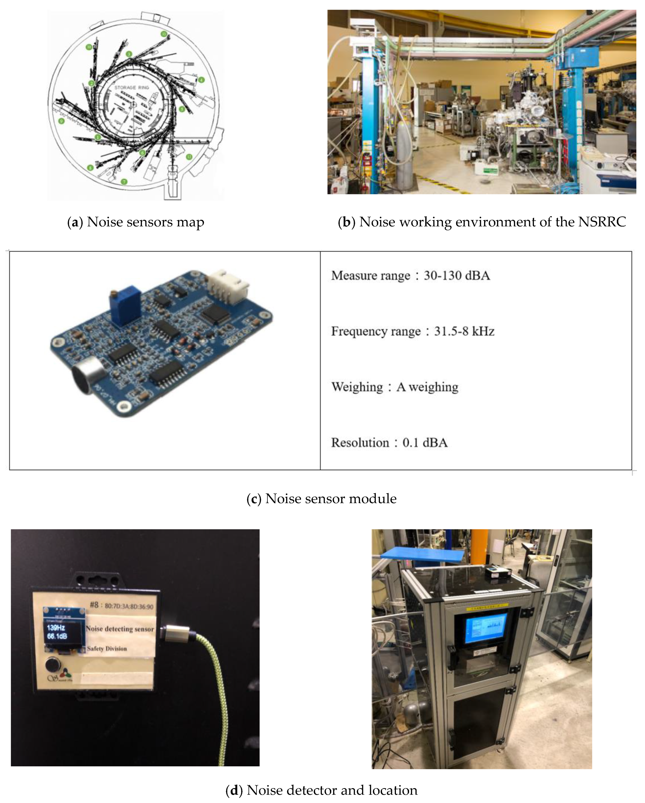
  • According to the data provided by the National Synchrotron Radiation Research Center (NSRRC), we performed daily and monthly statistical analyses on the noise data of 12 sensors at different frequencies. Once collected, the data were cleaned to derive useful information and analyze the data distribution.
  • We derived and extracted the features from the data analysis. We identified the frequency, time, and eight sensors from related history features, and then input a harmful frequency and the noisiest dBA sensor as extracted features.
  • We extracted the Leq historical features and time-related features from 80% of the data inputted to the machine learning model for training; the data for the remaining 20% was used for testing.

2. Materials

2.1. Information Introduction and Data Analysis

The noise data were provided by the NSRRC and contained more than 13,000,000 samples covering the time period from 08:00 on 1 February 2019 to 23:59 on 31 August 2019. The NSRRC installed 12 noise detection sensors around the work environment. As shown in Figure 2a, it showed the circle building has a 120 m circumference, and 24 straight line experimental stations that are differential function research experiments; the locations of the sensors were divided into the inner circle (1–6) and the outer circle (7–12), shown as green dots. In addition, there are many noise sources from vacuum pumps, cooling pumps, liquid nitrogen pressure relief, computer servers, etc. in the working environment, as shown in Figure 2b. In this study, the noise sensor module had more details including the measuring range, frequency range, weighing, and resolution, as shown in Figure 2c. This sensor device can instantly convert sound into Leq information in the cloud as shown in Figure 2d. Due to the limitations of the hardware and network, the Leq was recorded once per second and the average Leq was uploaded once every 10 s. Using this device, the different frequencies for Leq values were collected. The data were divided into eight different frequencies: 125 Hz, 250 Hz, 500 Hz, 1 kHz, 2 kHz, 4 kHz, 8 kHz, and 16 kHz. Furthermore, the noise monitoring system that provided sensors, the location, time and different frequency noise data are shown in Figure 2e. An alternative function in our monitoring system showed 12 groups for real-time linear charts that can be displayed within two hours’ data, as shown in Figure 2f. The segmentation for a maximum date interval of 12 group’s linear charts was set as a month, as shown in Figure 2g. Based on this system, we kept the data collection for further analysis in future work.
As the inner and outer ring sensors had different installation times, we divided the statistics of the Leq for the 12 sensors as shown in Figure 3. The data collected from sensors 1–6 were recorded from February to August; the remaining sensors collected data from April to August. The detailed time distribution and the number of data points are shown in Figure 3. In addition, all sensors had relatively complete data in July and August; thus, we used the most recent August data for training in the experiment.
Figure 4 shows the distribution of the average Leq levels of each sensor at 125 Hz and 1000 Hz over the different months (for the other monthly statistics from different frequencies, see Appendix A). It is evident that the average Leq level for sensor 8 was higher than that of the other sensors and closer to 70 dBA from 125 to 1000 Hz for each month. As shown in Figure 5, there was no sensor with a particularly prominent value from 2000~16 kHz, indicating that the low frequencies were the main noise sources in the environment. Therefore, we hypothesized that when the equipment was operating, it caused louder low-frequency noise near sensor 8. In fact, there were more noise sources near sensor 8 than in the other areas, which caused dBA values higher than those of the other sensors.
Next, we measured each sensor’s average daily data on a single frequency band over one week. The Leq value for the 125 Hz band was higher than that of the other frequencies, as shown in Figure 6 and Figure 7 (for the other daily statistics from different frequencies, see Appendix B). It has been established that the values for sensor 8 at 125 Hz–1000 Hz were obviously greater than those of the other sensors. In particular, it was evident that on Sunday, the sensor 8 Leq value was greater than the other days for all frequencies. We hypothesized that this was due to the fact that the equipment near sensor 8 was relatively old. In addition, there were no people working on Sunday and the temperature increased due to the air-conditioning being shut down to save energy costs. As a result, older equipment closer to sensor 8 were prone to make loud noises on Sunday. In addition, each sub-image in Figure 6 and Figure 7 had two lines, representing the average of the Leq levels of the 12 sensors in the morning (red) and at night (blue) within a week in the above frequency band. It is evident that as the frequency increased, the red line was higher than the blue line, and the differences between the average Leq levels during the morning and night also increased.
The results of statistical analyses for all sensor averages and for sensor 8 from morning and night differ from the Leq value at each frequency band over the week, as shown in Figure 8. The horizontal axis is the frequency and the vertical axis is the Leq error value. We can clearly observe that the average chart position for all sensors grows with increasing frequency in the range of 125 Hz to 16 kHz (apart from 500 Hz). When the frequency was higher, the difference was greater. Moreover, the average values for sensor 8 values were higher than those of all other sensors.
The results for all sensor values and from sensor 8 are shown in Figure 9, which shows a decrease in Leq levels with increasing frequency. On the other hand, there was an instance of low dBA levels from a high frequency. The results also show that all average sensors were lower than sensor 8 regardless of whether the levels were measured in the morning or at night. Thus, we can add features in the experiment.
The histograms added below show the average Leq changes in the morning and at night for each frequency band in a week where the upper and lower bounds of the vertical axis differ by 2.5 dBA. We can clearly see that the average noise in the morning was slightly higher than that measured at night on any frequency band. This gap was more obvious in Figure 10 and Figure 11 (see Appendix C for other noise frequency changes during the morning and night).

2.2. Methods

2.2.1. Feature Extraction

We derived and extracted features from the Leq time data for model training. The continuity of the noise generation process, which is affected by working days and working time, resulted in the input vector Xt containing temporal features; the output variable Yt+1 is the Leq value for the next minute. In this experiment, we chose to include days in a week, hours in a day, whether the day was a holiday, whether it was a Saturday or a Sunday, and the previous one minute or two minutes of historical noise frequency data for sensor 8. Thus, a total of 21-dimensional features were input for training (as shown in Table 1).

2.2.2. Machine Learning Model

Artificial intelligence has recently attracted considerable attention, and various machine learning approaches have been extensively implemented to model data in numerous applications [19,20]. For example, a travel time prediction model based on gradient boosting decision tree (GBDT) has been proposed to improve the prediction accuracy of traffic flow [21]. A new extreme gradient boosting (XGBoost) model with weather similarity analysis and feature engineering was proposed for short-term wind power forecasting [22]/ Air quality prediction in smart cities was undertaken using machine learning technologies based on sensor data [23]. This paper presented an innovative gradient boosting decision tree (GBDT) model to explore the joint effects of comprehensive factors on the traffic accident indicators [24]. A method was presented for predicting the broadband noise spectra of horizontal axis wind turbine generators [25] as well as a study on noise sensitivity by machine learning algorithms [26].
We used the gradient boosting model (GBM) to predict future Leq levels. This model combines fitting functions, loss functions, a decision tree, and gradient descent analysis [9]. The decision tree, error function L ( F ( X t ) , Y t + 1 ) [27,28], fitting function F(Xt) [29], and gradient descent analysis were applied to train the model. Specifically, the decision tree algorithm was used to generate a series of fitting functions F ( X t , β ) . The error function L ( F ( X t , β ) , Y t + 1 ) was used to calculate the fitting value F ( X t , β ) , which is the error from the actual value Yt+1, where Xt is the input vector at time t and Yt+1 is the output variable at time t+1. Next, we used the gradient descent method to find and select the fitting function F ( X t , β ) with the smallest error. The above steps are repeated until the optimal fitting function is found. The procedure is described in the equations in detail. The testing samples are put into the prediction model F(xt) to calculate the prediction results [8].
The objective of machine learning is to find a mapping function F(x) between the independent variable xi and target variable yi by using the training data. In order to find the optimal function, a loss function L(y, F(x)) is usually set for the model [21,25]. First, initialize the learning machine by the following equation:
F 0 ( X t ) = argmin β i = 1 N L ( y i , β )
where β is the estimated constant value that minimizes the loss function and N is the number of training samples.
Then, the target is to predict the next-24 h of noise Leq, where the output is the variable shown as yt+24. After N pairs of the input vector xt and the output variable yt+24 are given, a fitting function F(xt) is selected from unknown functions F(xt, β′) generated by the decision tree. Moreover, β′ is a gradient decent step size and ( x t i , y t + 24 i ) is the i-th training sample pair. When the value of the loss function L(yt+24, F(xt, β′)) is minimized as [8,21,25]
β = arg min β i = 1 N L ( y t + 24 i ,   F ( x t i , β ) )
the target function F(xt) is chosen as F(xt, β)
F 0 ( X t ) = F 0 ( x t , β 0 )
In this procedure, the value of N was 39,515. This is obtained from sensor 8 during August and the training model needed 80% of them. In addition, the gradient descent analysis is applied for optimized fitting function F(xt). The procedure is described as below. In the first step, the initial guess function F0(xt, β′) is produced and initial gradient descent step size β0 as [8,21,25]
β 0 = arg min β i = 1 N L ( y t + 24 i ,   F 0 ( x t i , β ) )
Thus, we take the gradient of loss function as a first-step base learner function f1(xt) as
f 1 ( x t ) = F 0 L ( y t + 24 ,   F 0 ( x t ) ) ,
β 1 = arg min β i = 1 N L ( y t + 24 i ,   [ F 0 ( x t i ) + β f 1 ( x t i ) ] )
In this study, M iterations was set as 500, where fm(xt) and βm are expressed as follows:
f m ( x t ) = F m 1 L ( y t + 24 ,   F m 1 ( x t ) )
β m = arg min β i = 1 N L ( y t + 24 i ,   [ F m 1 ( x t i ) + β f m ( x t i ) ] )
and the target function F(xt) is expressed as
F ( x t ) = F 0 ( x t ) + m = 1 M β m f m ( x t )
Through the above formulas, description flow was calculated by Algorithm 1, that is the entire GBM procedure. There is no doubt that F(xt) is the target prediction model, thus, the testing samples were put into the model to calculate the prediction results.
The algorithm flow is as follows:
Algorithm 1. GBM
Input:
1: F 0 ( x t , β 0 )
2: β 0 = arg min β 0 i = 1 N L ( y t + 24 i ,   F 0 ( x t i , β ) )
3: M: Iteration times
4: N: Number of data sets
Output: F( x t ) = F M ( x t )
5: For m = 1 to M
6: f m ( x t ) = F L ( y t + 24 ,   F m 1 ( x t ) )
7: β m = arg min β m i = 1 N L ( y t + 24 i , [ F m 1 ( x t i ) + β m . f m ( x t i ) ] )
8: F m ( x t ) = F m 1 ( x t ) + β m . f m ( x t )
9: end

3. Results and Discussion

To use the GBM model for future Leq value prediction on the 125 Hz frequency band, time characteristics and historical Leq were used as the input data. There were 12 sensor data, which were recorded every 10 s (sampling time = 10 s) with an average sample of 875,000. As the training time was too long, the sampling time was lengthened in order to reduce the amount of training data. Sensor 8 was used as a sampling example and used the previous two minutes of data to make predictions at different sampling times; the results are shown in Figure 12.
The X-axis in Figure 12 is the R2 [30], which represents the degree of curve fit between the predicted value and the actual value (sensor 8 at 125 Hz in August). The R2 value is distributed in the range of 0–1, and values closer to 1 indicate better prediction performance; otherwise, the prediction performance worsens. The Y axis is the RMSE [31]. Here, the higher the value indicates a worse prediction result; otherwise, the convergence is smaller. We found that a sampling time of 1 min and 30 s had a higher R2 and the best prediction performance; in addition, the RMSE was below 1 dBA. However, the R2 value of the 30 s sampling time was very close to those of 1 min and better, but the calculation requires double the time to complete. Thus, in the subsequent experimental design, the sampling time was adjusted to 1 min. Next, according to the frequency of harmful Leq levels at 125 Hz, a 21-dimensional feature prediction task was performed for the Leq for 12 sensors at this frequency in August. The features included the previous one minute and the previous two minutes of each frequency Leq value; the prediction results are shown in Figure 13.
In Figure 13, the X-axis represents the R2. The Y-axis represents the RMSE and the prediction results of 12 sensors at 125 Hz; R2 > 0.7 represents sensors 10, 8, and 3, among which sensor 3 had the largest R2 value and the smallest RMSE value. This indicates that input characteristics and Leq values are highly influence. In addition, the RMSE values of the 12 sensors were all below 1 dBA, indicating that the difference between the predicted Leq values and the actual Leq values was minute. Therefore, the R2 value was mainly used as an indicator to judge the quality of the prediction results. Observing the prediction results of sensor 1, not only was the R2 only 0.0643, but the RMSE was within 0.75 dBA and the input features were almost unrelated to the Leq values.
However, we added multiple linear regression (MLR) experiments to compare noise prediction results with the proposed approach, as shown in Figure 14a and Figure 15a. This shows that GBM outperforms MLR in terms of both index, R2, and RMSE while using the full 21 dimensions at 125 Hz. As shown in Figure 14b, the results clearly show that the GBM algorithm achieved higher R2 and showed a good grasp of the trend and reference value of noise fluctuations at each sensor, thus it was more effectively and accurate than MLR in this task. This result also shows that although the working environment was relatively stable, a very simple prediction model may not work well. This explains why we used the GBM prediction model for this problem in the NSRRC.
Furthermore, we compared three different input features set with 21, 16, and five dimensions, respectively, to investigate the impact of input factors. The conditions are shown in Table 1, and the prediction results in Figure 15a–c. Then, we clearly found more dimensions were better in terms of R2. Then, it was easily found that the input 21-dimensional data had better performance, as shown in Figure 15d. Therefore, the results showed that the full dimensional feature performed the best, indicating that the historical features may have more information than the time features. Thus, the more feature dimensions are input in the GBM enables efficient identification of suitable training features in response to reliable prediction results. Moreover, this study indicates that the loudest location near the working environment was sensor 8, and 125 Hz was the most serious harmful frequency. For the practical issues, we could pre-improve the low frequency pump surrounding sensor 8 by using sound insulators or remind workers to prevent long-term exposure in that area.
We counted the prediction results of all sensors with a R2 greater than 0.7 at all frequencies, as shown in Table 2. Taking sensor 2 as an example, the R2 of noise with a frequency of 500 Hz and with a frequency of 1 kHz were both greater than 0.7 (marked with an asterisk). Other sensors can be deduced by analogy from the prediction results at different frequencies, as shown in Figure 16.
Here, we focused on the noise value of 125 Hz as its dBA values reached levels that are harmful to the human body [15,16,17,18]. Moreover, we found that sensors 3, 8, and 10 achieved favorable prediction performance, as shown in Table 2. Among them, the prediction performance of sensor 3 from 125 Hz to 4 kHz showed a R2 greater than 0.7, and these noise frequencies were coherent with one another. Likewise, the sensor 7 noise frequencies between 2 kHz and 16 kHz were coherent with one another.
As a result, we found that while the sensor prediction index R2 of this frequency was above 0.7, the values near this frequency could also produce excellent prediction results (for example, 500 Hz and 1000 Hz of sensor 2, 125 Hz to 4 kHz of sensor 3, 500 Hz and 1000 Hz of sensor 4, and 500 Hz and 1000 Hz of sensor 6). Thus, we found mutual influence between similar frequencies and hypothesized that the noise sources of similar frequencies were likely to have very similar occurrence conditions. The coefficient of determination (R2) of the sensor was higher than 0.7, and the root-mean-square-error (RMSE) was less than 1 dBA. This indicates that the proposed model could accurately predict the trends of future Leq levels with an average error margin within 1 dBA. Therefore, we successfully completed predictions for all sensors at other noise frequencies, and derived an effective reference value for improving future prediction accuracy.

4. Conclusions

In this study, we found that as frequencies increased, the average Leq error values between morning and night were greater, with noise in the morning returning higher and greater values than those at night. This may be due to the fact that more people work in the morning and more noise is generated. Moreover, the human voice has a high noise frequency, whereas machine pumps have a noise lower frequency, indicating significant differences in noise sources.
This study focused on the prediction results for the noise frequency for one of twelve sensors (sensor 8) at 125 Hz. This sensor was chosen because its static Leq value (>70 dBA) reached the threshold of damaging human hearing, which affects physical and mental health. Based on this finding, we used the GBM model to predict future noise data. The Leq prediction results for sensor 8 at 125 Hz showed an error rate of less than 1 dBA and a R2 value greater than 0.7, which is a favorable prediction performance result. The poorer prediction results of the other sensors were between 2 to 1 dBA with a R2 value that was generally below 0.7.
The results indicate that the prediction model worked well in most regions and frequencies and particularly for sensor 8 (125 Hz), which is a serious noise zone. The results also indicate that this working environment produced good noise prediction performance using the proposed method. This enables the notification of laborers to prevent long-term exposure while predicting future noise pollution. In fact, we are now collecting more characteristic data for several months for this purpose. We believe that it would be better to have a longer observation duration to predict detailed noise location. This would keep employees healthy for avoiding a harmful noise position to prevent people from working in that environment. In the future, we will analyze the data structures of the noise frequencies of more sensors, discuss noise types, and analyze the possibilities of noise-related physical harm. We will also attempt to add new features to improve noise prediction performance.

Author Contributions

P.-J.W. wrote and conducted the experiments, analyzed the results, and organized the layout of the paper, figures, and tables. C.H. conceived and corrected the article and was responsible for making clear and understandable content. All authors reviewed the manuscript. All authors have read and agreed to the published version of the manuscript.

Funding

This research was funded by National Synchrotron Radiation Research Center (NSRRC), grant number 10811SAO01.

Acknowledgments

The authors acknowledge the financial support and equipment provided by the National Synchrotron Radiation Research Center (NSRRC), Taiwan. We gratefully acknowledge the software support of PTCOM Technology Co. Ltd.

Conflicts of Interest

The authors declare no conflict of interest.

Appendix A

Average at different frequencies in different months for different sensors.
Applsci 10 06619 i0a1

Appendix B

Daily average at different frequencies per week for different sensors.
Applsci 10 06619 i0a2

Appendix C

Average morning vs. night in a week for all sensors.
Applsci 10 06619 i0a3

References

  1. Goines, L.; Hagler, L. Noise pollution: A modern plague. South. Med. J. 2007, 100, 287–294. [Google Scholar] [CrossRef]
  2. Pirrera, S.; Valck, E.D.; Cluydts, R. Nocturnal road traffic noise: A review on its assessment and consequences on sleep and health. Environ. Int. 2010, 36, 492–498. [Google Scholar] [CrossRef] [PubMed]
  3. Effects of Noise on Health. Available online: https://ncs.epa.gov.tw/noise/B-04-01.html (accessed on 25 May 2020).
  4. Shen, D.H.; Wu, C.M.; Du, J.C. Application of grey model to predict acoustical properties and tire/road noise on asphalt pavement. In Proceedings of the 2006 IEEE Intelligent Transportation Systems Conference, Toronto, ON, Canada, 17–20 September 2006; pp. 175–180. [Google Scholar]
  5. Cheng, Y.; Ying, C. Simplifying prediction method for traffic noise based on FHWA traffic noise model. In Proceedings of the 2011 International Symposium on Water Resource and Environmental Protection, Xi’an, China, 20–22 May 2011; pp. 2665–2667. [Google Scholar]
  6. Zhang, R.; Wang, H.I. Nonlinear prediction of gross industrial output time series by Gradient Boosting. In Proceedings of the 2011 IEEE 18th International Conference on Industrial Engineering and Engineering Management, Changchun, China, 3–5 September 2011; pp. 153–156. [Google Scholar]
  7. Sangani, D.; Erickson, K.; Hasan, M.A. Predicting Zillow estimation error using linear regression and gradient boosting. In Proceedings of the 2017 IEEE 14th International Conference on Mobile Ad Hoc and Sensor Systems (MASS), Orlando, FL, USA, 22–25 October 2017; pp. 530–534. [Google Scholar]
  8. Lee, M.; Lin, L.; Chen, C.Y.; Tsao, Y.; Yao, T.H.; Fei, M.H.; Fang, S.H. Forecasting Air Quality in Taiwan by Using Machine Learning. Sci. Rep. 2020, 10, 4153. [Google Scholar] [CrossRef] [PubMed]
  9. Friedman, J.H. Greedy function approximation: A gradient boosting machine. Ann. Stat. 2001, 29, 1189–1232. [Google Scholar] [CrossRef]
  10. Islam, S.; Kalita, K. Assessment of traffic noise in Guwahati city, India. Int. Res. J. Eng. Technol. 2017, 4, 3335–3339. [Google Scholar]
  11. Benocci, R.; Bellucci, P.; Peruzzi, L.; Bisceglie, A.; Angelini, F.; Confalonieri, C.; Zambon, G. Dynamic noise mapping in the Suburban area of Rome (Italy). Environments 2019, 6, 79. [Google Scholar] [CrossRef] [Green Version]
  12. Garcia, J.S.; Solano, J.J.P.; Serrano, M.C.; Camba, E.A.N.; Castell, S.F.; Asensi, A.S.; Suay, F.M. Spatial statistical analysis of urban noise data from a WASN gathered by an IoT system: Application to a small city. Appl. Sci. 2016, 6, 380. [Google Scholar] [CrossRef]
  13. Chang, T.Y.; Beelen, R.; Li, S.F.; Chen, T.I.; Lin, Y.J.; Bao, B.Y.; Liu, C.S. Road traffic noise frequency and prevalent hypertension in Taichung, Taiwan: A cross-sectional study. Environ. Health 2014, 13, 37. [Google Scholar] [CrossRef] [Green Version]
  14. Subramaniam, M.; Hassan, M.Z.; Sadali, M.F.; Ibrahim, I.; Daud, M.Y.; Aziz, S.A.; Samsudin, N.; Sarip, S. Evaluation and analysis of noise pollution in the manufacturing industry. J. Phys. Conf. Ser. 2019, 1150, 012019. [Google Scholar] [CrossRef] [Green Version]
  15. Baliatsas, C.; Kamp, I.V.; Poll, R.V.; Yzermans, J. Health effects from low-frequency noise and infrasound in the general population: Is it time to listen? A systematic review of observational studies. Sci. Total Environ. 2016, 557–558, 163–169. [Google Scholar] [CrossRef] [Green Version]
  16. Lee, H.P.; Wang, Z.; Lim, K.M. Assessment of noise from equipment and processes at construction sites. Build. Acoust. 2017, 24, 21–34. [Google Scholar] [CrossRef]
  17. Reybrouck, M.; Podlipniak, P.; Welch, D. Music and Noise: Same or Different? What Our Body Tells Us. Front. Psychol. 2019, 10, 1153. [Google Scholar] [CrossRef] [PubMed]
  18. Liu, C.; Ding, D.; Zhu, Y.; Wang, H.; Cheng, X.; Zhao, Z.; Cao, J.; Zhai, S.; Yu, N. Auditory characteristics of noise-exposed memberscrossing age-related groups. J. Otol. 2018, 13, 75–79. [Google Scholar]
  19. Fang, S.H.; Chang, W.H.; Tsao, Y.; Shih, H.C.; Wang, C. Channel State Reconstruction Using Multilevel Discrete Wavelet Transform for Improved Fingerprinting-Based Indoor Localization. IEEE Sens. J. 2016, 16, 7784–7791. [Google Scholar] [CrossRef]
  20. Fang, S.H.; Yang, Y.H.S. The Impact of Weather Condition on Radio-based Distance Estimation: A Case Study in GSM Networks with Mobile Measurements. IEEE Trans. Veh. Technol. 2016, 65, 6444–6453. [Google Scholar] [CrossRef]
  21. Cheng, J.; Li, G.; Chen, X. Research on Travel Time Prediction Model of Freeway Based on Gradient Boosting Decision Tree. IEEE Access 2019, 7, 7466–7480. [Google Scholar] [CrossRef]
  22. Zheng, H.; Wu, Y. A XGBoost Model with Weather Similarity Analysis and Feature Engineering for Short-Term Wind Power Forecasting. Appl. Sci. 2019, 9, 3019. [Google Scholar] [CrossRef] [Green Version]
  23. Iskandaryan, D.; Ramos, F.; Trilles, S. Air Quality Prediction in Smart Cities Using Machine Learning Technologies Based on Sensor Data: A Review. Appl. Sci. 2020, 10, 2401. [Google Scholar] [CrossRef] [Green Version]
  24. Wu, W.; Jiang, S.; Liu, R.; Jin, W.; Ma, C. Economic development, demographic characteristics, road network and traffic accidents in Zhongshan, China: Gradient boosting decision tree model. Transp. A Transp. Sci. 2020, 16, 359–387. [Google Scholar] [CrossRef]
  25. Grosveld, F.W. Prediction of Broadband Noise from Horizontal Axis Wind Turbines. J. Propuls. 1984, 1, 292–299. [Google Scholar] [CrossRef]
  26. Kalapanidas, E.; Avouris, N.; Craciun, M.; Neagu, D. Machine Learning algorithms: A study on noise sensitivity. In Proceedings of the 1st Balkan Conference in Informatics, Thessaloniki, Greece, 21–23 November 2003; pp. 356–365. [Google Scholar]
  27. White, G.C.; Bennetts, R.E. Analysis of frequency count data using the negative binomial distribution. Ecology 1996, 77, 2549–2557. [Google Scholar] [CrossRef]
  28. Matheson, I.B.C. A critical comparison of least absolute deviation fitting (robust) and least squares fitting: The importance of error distributions. Comput. Chem. 1990, 14, 49–57. [Google Scholar] [CrossRef]
  29. Buckley, J.; James, L. Linear regression with censored data. Biometrika 1979, 66, 429–436. [Google Scholar] [CrossRef]
  30. Nagelkerke, N.J.D. A note on a general definition of the coefficient of determination. Biometrika 1991, 78, 691–692. [Google Scholar] [CrossRef]
  31. Willmott, C.J.; Matsuura, K. Advantages of the mean absolute error (MAE) over the root mean square error (RMSE) in assessing average model performance. Clim. Res. 2005, 30, 79–82. [Google Scholar] [CrossRef]
Figure 1. The main process of the method in three parts.
Applsci 10 06619 g001
Figure 2. (a) Noise sensor map. (b) Noise working environment of the National Synchrotron Radiation Research Center (NSRRC). (c) Noise sensor module. (d) Noise detector and location. (e) Noise monitoring system illustrating. (f) Two hours’ real-time detection chart. (g) One-month detection chart.
Applsci 10 06619 g002aApplsci 10 06619 g002b
Figure 3. Twelve noise sensors collected data in different months.
Applsci 10 06619 g003
Figure 4. Average at 125 Hz and 1000 Hz in different months for different sensors.
Applsci 10 06619 g004
Figure 5. Different sensor averages at 2000 Hz and 16,000 Hz for different months.
Applsci 10 06619 g005
Figure 6. Daily average at 125 Hz and 1000 Hz in one week for different sensors.
Applsci 10 06619 g006
Figure 7. Daily average at 2000 Hz and 16,000 Hz in one week for different sensors.
Applsci 10 06619 g007
Figure 8. Morning and night noise error data vs. frequency (all sensor avg. vs. sensor 8).
Applsci 10 06619 g008
Figure 9. Morning and night average noise data vs. frequency (all sensor avg. vs. sensor 8).
Applsci 10 06619 g009
Figure 10. Average morning vs. night at 125 Hz and 1000 Hz in a week for all sensors.
Applsci 10 06619 g010
Figure 11. Average morning vs. night at 2000 Hz, 16000 Hz in a week for all sensors.
Applsci 10 06619 g011
Figure 12. Different sampling times vs. predicted effect.
Applsci 10 06619 g012
Figure 13. Predicted effect at 125 Hz for different sensors.
Applsci 10 06619 g013
Figure 14. (a) Performance of multiple linear regression (MLR) method. (b) Combine MLR and gradient boosting model (GBM).
Applsci 10 06619 g014
Figure 15. (a) Performance of input features set with 21 dimensions. (b) Performance of input features set with 16 dimensions. (c) Performance of input features set with five dimensions. (d) Performance of input features set with three combined kinds of different dimensions.
Applsci 10 06619 g015
Figure 16. Different sensor prediction effects at different frequencies.
Applsci 10 06619 g016
Table 1. Input features obtained from noise sensor monitoring.
Input Feature (21-Dimensional)
History featureprevious 1 min of sensor * 8previous 2 min of sensor * 816
Time featureWhich day in a week, Which hour in a day, Holiday or not, Saturday or not, Sunday or not.5
* Eight noise frequencies: 125 Hz, 250 Hz, 500 Hz, 1 kHz, 2 kHz, 4 kHz, 8 kHz, and 16 kHz.
Table 2. All sensors with R2 greater than 0.7 at all frequencies.
Frequency (Hz)1252505001k2k4k8k16k
Sensor1
( R 2 > 0.7 )
Sensor2
( R 2 > 0.7 )
Sensor3
( R 2 > 0.7 )
Sensor4
( R 2 > 0.7 )
Sensor5
( R 2 > 0.7 )
Sensor6
( R 2 > 0.7 )
Sensor7
( R 2 > 0.7 )
Sensor 8
( R 2 > 0.7 )
Sensor9
( R 2 > 0.7 )
Sensor10
( R 2 > 0.7 )
Sensor11
( R 2 > 0.7 )
Sensor12
( R 2 > 0.7 )
★ The R2 of noise with a frequency greater than 0.7.

