GPU Parallel Implementation for Real-Time Feature Extraction of Hyperspectral Images

Featured Application

This work contributes to the real-time processing of UAV hyperspectral imaging.

Abstract

As the application of real-time requirements gradually increases or real-time processing and responding become the bottleneck of the task, parallel computing in hyperspectral image applications has also become a significant research focus. In this article, a flexible and efficient method is utilized in the noise adaptive principal component (NAPC) algorithm for feature extraction of hyperspectral images. From noise estimation to feature extraction, we deploy a complete CPU-GPU collaborative computing solution. Through the computer experiments on three traditional hyperspectral datasets, our proposed improved NAPC (INAPC) has stable superiority and provides a significant speedup compared with the OpenCV and PyTorch implementation. What’s more, we creatively establish a complete set of uncrewed aerial vehicle (UAV) photoelectric platform, including UAV, hyperspectral camera, NVIDIA Jetson Xavier, etc. Flight experimental results show, considering hyperspectral image data acquisition and transmission time, the proposed algorithm meets the feature extraction of real-time processing.

1. Introduction

Hyperspectral images (HSIs) can simultaneously obtain two-dimensional spatial information and one-dimensional spectral information of the scene. They have very high spectral resolution and can detect more precise ground object features. HSIs are widely used in a variety of tasks, such as anomaly detection [1], scene change detection [2], and classification [3,4,5]. Nowadays, uncrewed aerial vehicle (UAV) based hyperspectral imaging is also a relatively new remote sensing technology [6], which is widely used in agriculture and forestry, such as the estimation of plant potassium accumulation [7], yield evaluation [8], and vegetation classification [9]. Among these, the classification of HSIs has become the focus of numerous research efforts, since it plays a significant role in the fields of resource environment [10], food production [11], clinical application [12], and defense security [13]. Each pixel is assigned a label’s number for a specific class, and the classification of HSIs aims to assign a unique label for each test pixel in the scene. To achieve this, many classifiers have been proposed or applied to the hyperspectral classification field in the past ten years, such as the support vector machine (SVM) [14], spectral gradient, spatial random forest, and neural networks [15,16].

However, according to the characteristics of pixel-by-pixel-multi-band of HSIs and data redundancy between bands, the processing of raw data in the classifier will bring huge computational overhead, which brings pressure to the real-time characteristics of image processing and affects the accuracy of classification, especially on mobile platforms, such as UAV. Thus, feature extraction (FE) is an important technique for HSIs data processing [17]. Many FE methods have been developed in recent years. Hyperspectral image feature extraction mainly includes linear FE methods and non-linear FE methods. Typical linear FE methods include principal components analysis (PCA) [18], linear discriminant analysis (LDA) [19], independent component analysis (ICA) [20], and maximum noise fraction (MNF) [21]. Non-linear FE methods are mainly based on manifold learning [22], graph theory, and kernel transformation. The linear FE methods are usually easy to implement and explain in practice, especially in some image classification tasks with extensive real-time search. On the other hand, high-performance computing (HPC) in hyperspectral image applications has also become a research focus for HSIs data processing [23,24,25]. However, the current parallel algorithms are mostly based on computer simulation.

In this article, a flexible and efficient method is utilized in the noise adaptive principal component (NAPC) algorithm, specifically based on compute unified device architecture (CUDA). From noise estimation to feature extraction, we establish a complete CPU-GPU collaborative computing solution, which implements different CUDA parallelization key kernels and use some GPU programming optimization methods to achieve the maximum acceleration effect. Experiments show that the classification effect of the improved NAPC (INAPC) has stable superiority compared with other methods and provides a significant speedup compared with the OpenCV and PyTorch implementation. What’s more, since most of the parallel algorithms are based on computer simulations, we conduct constructive and innovative flight experiments. We establish a complete set of UAV photoelectric platform, including UAV, hyperspectral camera, NVIDIA Jetson Xavier (AGX, Changsha, China), etc. Flight experimental results show, considering hyperspectral image data acquisition and transmission time, the proposed algorithm meets the feature extraction of real-time processing.

The rest of this article is structured as follows. In Section 2, the INAPC algorithm is presented. Section 3 describes our parallel implementations and optimization methods in detail. Section 4 shows and discusses the results in terms of both computer simulation and flight experiments. The conclusions and future work are presented in Section 5.

2. Hyperspectral Image Feature Extraction Based on INAPC

Aiming at transforming the original hyperspectral image data into a feature space, PCA obtains the principal component information according to the magnitude of the variance, while NAPC determines the principal component information by the magnitude of the signal-to-noise ratio, which reduces the influence of noise, but needs external noise processing [26]. This method is essentially an overlap operation of two PCA, which means more massive computational overhead taking account of the characteristics of hyperspectral data, as stated above.

The INAPC algorithm, also considered as a complete CPU-GPU collaborative computing solution, mainly whitens the noise in each band before performing the principal component analysis, so we directly deploy two singular value decompositions (SVDs) on the noise whitening process and the adjusted observation matrix (the data after noise reduction), which can reduce calculation steps and eliminate uneven noise distribution. In the noise whitening process, the noise covariance matrix calculation is a key step, so we put the noise estimation into the entire data processing, where noise is estimated by the minimum/maximum autocorrelation factors method (MAF) [21]. After the second SVD for the adjusted observation matrix, we propose a choosing rule to determine the k value (the number of principal components).

Spectral feature extraction is also a process of dimensionality reduction. Through the choosing rule, a clear superiority is established that there is no need to manually input the value of k or set it to a fixed value on different input data anymore, so we can more adaptively and flexibly perform feature extraction on different hyperspectral datasets, which is also more conducive to the deployment of real-time applications.

The details of our choosing rule are as follows. At first, put all singular values into a vector $V=\left[{\sigma }_1,{\sigma }_2,\cdots ,{\sigma }_r\right]$, and calculate the gradient vector G of the singular value vector V, denote $G=\left[g_1,g_2,\cdots ,{\sigma }_r\right]$. Then, we find the first ${\sigma }_k$ while satisfying the following choosing rules:

$$1-\frac{{\sigma }_k}{{\sigma }_1}\ge 94\%\&\&\frac{g_k}{g_1}\le 1\%$$

(1)

The fixed values 94% and 1% are derived by mathematical induction based on eigenvalue and accuracy [27,28]. Algorithm 1shows the pseudocode and the annotations of the INAPC algorithm, and the calculation matrix of each step are described in Algorithm 1. The fourth step is noise estimation. ${∆}_1$ and ${∆}_2$ represent the neighborhood estimation in the horizontal and vertical directions, respectively. Since the hyperspectral image can consider as a three-dimensional data cube (which has been reshaped to a two-dimensional matrix), a three-layer loop needs to be set up.

Algorithm 1: Improved noise adaptive principal component (INAPC) algorithm.

1  INPUT: hyperspectral image $X$ 2 1: reshape the raw data to matrix X [row*col, band] 3 band: band numbers; row, col: spatial dimensions 4 2: centralization matrix: 5  for k = 1: band 6  ${\overline{X}}_k$; 7  $T=X_k-{\overline{X}}_k$; 8  end 9 3: covariance matrix: $S=\frac{1}{\mathrm{row}\ast \mathrm{col}-1}{T}^{T}T$; 10 4: noise estimation: 11  for t = 0: row 12 for i = 1: col 13 for j = 0: band 14 ${∆}_1\left[i+t\ast col,j\right]=X\left[i+t\ast col,j\right]-X\left[i+t\ast \left(col-1\right),j\right]$ 15 end 16 end 17 end 18 for t = 0: row – 1 19 for i = 0: col 20 for 0 = 1: band 21 ${∆}_2\left[i+t\ast col,j\right]=X\left[i+t\ast col,j\right]-X\left[i+\left(t+1\right)\ast col,j\right]$ 22 end 23   end 24  end 25  final: $\mathrm{N}=({∆}_1+{∆}_2)/2$; 26 5: for k = 1: band 27 ${\overline{N}}_k$; 28  $T_N=N-{\overline{N}}_k$; 29  end 30 6: $C_N=\frac{1}{\mathrm{row}\ast \mathrm{col}-1}{T}_N{}^T{T}_N$; 31 7: apply 1st SVD to $C_N$, and get $U_N,{{{\displaystyle \sum }}^{}}_N,V_N^T$; 32 8: noise whitening matrix: $W=U_N\frac{1}{\sqrt{{{{\displaystyle \sum }}^{}}_N}}$; 33 9: adjusted observation matrix: $C_D=WS{W}^T$; 34 10: apply 2nd SVD to $C_D$, and get $U_D,{{{\displaystyle \sum }}^{}}_D,V_D^T$; 35 11: choose the rank value k based on choosing rule; 36 12: cut off the SVD results $U_k$ based on k; 37 13: $P=W{U}_k$; 38  OUTPUT: feature extraction result $\mathit{Y}={\mathit{P}}^{\mathit{T}}\mathit{X}$

3. GPU Parallel Implementation Based on CUDA

The proposed parallel implementation starts with the characteristics of GPU programming. Matrix operations are always performed by the GPU, and the memory transfer between the CPU (host) and the GPU (device) is reduced as much as possible. A few critical parallel steps and optimization strategies will be shown next.

3.1. Reduction

The reduction is a typical parallel algorithm that uses a binary compound combination law operator to generate $O\left(1\right)$ results for the incoming $O\left(N\right)$ input data. In addition, one of CUDA’s efficient strategies is the use of shared memory. When one block starts executing, GPU will allocate a certain amount of shared memory, and the address space of shared memory will be shared by all threads in the block, which can significantly reduce the global memory bandwidth required by the kernel.

According to a large amount of hyperspectral data, we set up a two-level reduction for the calculation of the sum of each column of the matrix. When inputting a matrix of $M$ rows and $N$ columns ($M>>N$), each thread loads one element from global to shared memory. For first level reduction block, which is specified by $dim3dimBlock\left(block1,1\right)$, there are threads whose number is block1, so that the grid dimension can be calculated as,

$$dim3dimGrid\left(\left(N/\left(block1\right)\right)+\left(!\left(N\%\left(block1\right)\right)?0:1\right),M\right)$$

(2)

Here, we allocate memory for first level reduction results, $r1$ is a static floating-point pointer,

$$staticintr1size=dimGrid.x\ast dimGrid.y$$

(3)

$$cudaMalloc\left(\left(void\ast \ast \right)\&r1,sizeof\left(float\right)\ast r1size\right)$$

(4)

Then, we perform the second level reduction on the results of the first level with the pointer r1 as input. Threads organization of the second level reduction can be set as,

$$dim3dimBlock2\left(block2,1\right)$$

(5)

$$dim3dimGrid2(\left(dimGrid.x/\left(block2\right)\right)+\left(!\left(dimGrid.x\%\left(block2\right)\right)?0:1\right),M$$

(6)

The design using two-level reduction can effectively improve the calculation efficiency when considering large hyperspectral data and limited shared memory resources.

3.2. Matrix Operations

For floating-point matrix-matrix/vector multiplication, we directly deploy the cuBLAS-SGEMM library in function. One of these functions is shown in Figure 1. The formal parameter in the function is the previously defined matrix structures, including the matrix parameters, such as matrix header pointers and dimensions.

We initialize cuBLAS with library function $cublasInit()$ and close cuBLAS with library function $cublasShutdown()$ in the context of these wrapped functions. In addition, the selection of SGEMM parameters in the function can transpose the original matrix before multiply operation.

3.3. Noise Estimation

Noise estimation is an essential part of our proposed algorithm, and the calculation formulas are step 4 in Algorithm 1, which uses different neighborhood information to estimate each pixel. We still set each thread to load one element from global memory and set the size of blocks to the number of bands, which means that one block contains all the band data values of one pixel. In this way, the grid dimension can be set as the spatial dimension,

$$dim3dimBlock\left(band\right)$$

(7)

$$dim3dimGrid\left(row,col\right)$$

(8)

Figure 2 shows the detail of threads organization of noise estimation. As shown in Figure 2, a small spectral cube (marked in yellow on the left) corresponds to a pixel in the spatial dimension, this cube corresponds to one block in the grid, and each thread in this block corresponds to the band values of the pixel.

3.4. SVD

In some other parallel processing of the hyperspectral image, GPU acceleration is mostly performed only for matrix operations [29] or using the CPU computing library for feature decomposition [30]. In our algorithm, we will perform feature decomposition in GPU based on the cuSolver library and reduce data transfer between the host and the device as much as possible.

The basic use of cuSolver to implement the SVD computation is reported in the official library documentation [31]. Different from the steps in the official documentation, we don’t need to create all the parameter pointers and their corresponding memory here, because they have been declared or completed in the previous context. Besides, the input data and results of the calculation don’t have to be transferred between host and device, and we only need to use part of the calculated value. What more, encapsulating SVD into a class helps us to call it multiple times, and we can dynamically choose whether to return the host or continue the calculation in the device without having to reconstruct the context of the complete calculation function multiple times, thereby reducing time consumption. In addition, this approach is also very conducive to the migration of our algorithm.

We show the simplified SVD parallel code in Algorithm 2. The first step is to set up the SVDT class and declare its constructor, destructor, calculation function, and private parameters. When a new object of the SVDT class is created, the constructor is executed. As shown in step 2, the parameters m and n are the dimensions of the matrix to be decomposed. We only need to initialize the cuSolverDN library and calculate the size of the work buffers needed here. Step 3 is the execution of the calculation function, and no data transfer operation is required here. The fourth step is the execution of the destructor, which is used to release temporary memory and useless pointers. Function $get\_p$ is used to call the function pointer to facilitate debugging and verify the results.

Algorithm 2: SVD parallelization.

1 1: set class $SVDT${ 2 $public:SVDcompute\left(args\right)$; 3    $~SVDT()$; 4    $SVDT\left(constintm,constintn\right)$; 5                     $float\ast get\_p\left(void\right);$ 6 $private:cublas\_status;\dots \dots float\ast d\_work=NULL;\dots \dots$ 7 } 8 2: $SVDT::SVDT\left(constintm,constintn\right)${ 9 $cusolverDnCreate\left(\&cusolverH\right)$; 10 $cusolverDnSgesvdbufferSize\left(cusolverH,m,n,\&lwork\right)$; 11 } 12 3: $SVDT::SVDcompute${ 13 $cudaEventCreate\left(\&startEvent\right);$ 14 $cusolverDnSgesvd\left(args\prime \right);$ 15 $cudaEventRecord\left(stopEvent\right);$ 16 $cusolverDnDestroy\left(cusolverH\right);$ 17 } 18 4: $SVDT::~SVDT();$

3.5. Summary

According to the analysis above, we construct related functions corresponding to each computing operation requirement, as shown in

Table 1. Key functions or class and their relative annotation.

No.	Functions/Class	Annotation
1	void read_matrix(matrix* A, char* file)	Read matrix in from file, store in row-major order, *A must point to an uninitialized matrix
2	void copy_matrix_to_device(matrix* A)	typedef struct $matrix$, matrix dimensions are in member $dim[]$
3	void create_matrix_on_device(matrix* A, int rows, int cols, float value)	malloc cuda space to hold temp matrices
4	void matrix_multiply_d(matrix a, matrix b, matrix c)	SGEMMS, Matrix multiplication, $c=a\ast b$
5	void matrix_multiply_AtB_d(matrix a, matrix b, matrix c)	SGEMMS, Matrix multiplication, $c=a^T\ast b$; $c=a\ast b^T$
6	void matrix_sub_d(matrix a, matrix b, int block_size)	Matrix subtraction
7	void sum_cols_d(action_t action, matrix a, matrix c, int* params)	Average and sum with reduction
8	int choose_rank(float *a, int m)	Select the number of principal components of dimensionality reduction
9	void n_estimate_d(matrix a, matrix b, int block_size,int row,int col)	Noise estimation for the construction of noise covariance matrix $C_N$
10	SVDT svd(row, col); svd.SVDcompute(args)	SVD

* represents a pointer in the C++ language.

. Figure 3 shows the flowchart of the proposed INAPC algorithm parallel implementation. In Figure 3, the calculation process of each step in Algorithm 1 is displayed clearly. There are four main data transfer between host and device, whose direction and corresponding data are marked in red. Their time consumption and proportion will be discussed in detail in Section 4.

4. Experimental Setup and Materials

Experiments of the proposed method will be performed firstly on a personal computer equipped with Intel CPU and NVIDIA GPU. The detailed features of this platform are listed in

Table 2. Hardware specification of the CPU and GPU.

CPU	Processor Type	IntelI CoITM) i7-9750H
	Number of Cores	6cores × 2
	Processor Base Frequency	2.60 GHz
	Main Memory	8 GB
	L3 cache	12 MB
GPU	Product Series	GeForce GTX 1650
	CUDA Driver Version Runtime Version	10.2/10.0
	CUDA Capability Major/Minor version number	7.5
	(16) Multiprocessors, (64) CUDA Cores/MP	1024 CUDA Cores
	GPU Max Clock rate	1560 MHz (1.56 GHz)
	Total amount of shared memory per block	49,152 bytes
	Max dimension size of a thread block (x, y, z)	(1024, 1024, 64)

. Besides, software specifications of the considered platform consist of Microsoft Visual Studio 2017 Compiler (Community Edition, Changsha, China), CUDA 10.0 (Ubuntu 16.04, Changsha, China) and OpenCV 3.0 (Changsha, China), etc.

Three real traditional hyperspectral datasets are tested in our experiments: Indian Pines, Salinas scene, Pavia University scene. Their details are given in

Table 3. Details of the three experimental hyperspectral images.

SCENE	Indian Pines	Salinas Scene	Pavia University Scene
Instruments	AVIRIS sensor	AVIRIS sensor	ROSIS sensor
Wavelength Range (μm)	$0.4-2.5$	$0.4-2.5$	$0.43-0.86$
Size	145 × 145 × 220	512 × 217 × 224	610 × 340 × 103
Spatial Resolution (m)	20	3.7	1.3
Ground-truth classes	16	16	9

.

For the UAV experiments, the most critical parts of the UAV photoelectric platform are the UAV (a DJI Jingwei M600 PRO, Changsha, China), the hyperspectral camera (SPECIM_FX17E, Changsha, China), and the computing development board (NVIDIA Jetson Xavier, AGX, Changsha, China). The hardware configuration and parameters of the latter two are given in

Table 4. Main parameters of the SPECIM_FX17E snapshot hyperspectral sensor.

Specification	Value	Specification	Value
Wavelength Range	935–1720 nm	Spectral Resolution	3.5 nm@1129 nm
Sample	640	Digitization	12 bit
Lines	482	Horizontal Field Angle	38°
Bands	224	Spatial Resolution	0.32 (300 m)
Single Shooting Speed	5 s	Operating Voltage	12 V

and

Table 5. Several key technical specifications of NVIDIA Jetson AGX Xavier module.

NVIDIA Jetson AGX Xavier
GPU	NVIDIA Volta architecture with 512 NVIDIA CUDA cores
CPU	8-Core Carmel ARM v8.2 64-Bit CPU, 8 MB L2 + 4 MB L3
Memory	32 GB 256-Bit LPDDR4x 2133 MHz—136.5 GB/s
Size	87 mm × 100 mm

, respectively.

5. Results and Discussion

5.1. Feature Extraction

As stated above, the choosing rule aims to adaptively determine the number of principal components of feature extraction, which is also the dimension k after dimension reduction. The appropriate selection of k value allows us to express more information with fewer components. Figure 4 shows the eigenvalue curves of three hyperspectral datasets. The positions of the dotted lines represent the selected k values of the three datasets under the choosing rule.

It shown in Figure 4, that the choosing rules make the selected k of the three datasets fall in the region where the k value is very small and basically does not change, which means that the first k principal components represent enough data information.

Then we evaluate the choosing rules from the perspective of classification effect and verify the validity of feature extraction, where we choose CMR-SVM [32] for the classifier. As for the classification effect, several metrics have been used to measure the classification accuracies [33]. Accuracy is essentially a measure of how many ground truth pixels were classified correctly (in percentage), average accuracy (AA) is the average of the accuracies for each class, and overall accuracy (OA) is the accuracy of each class weighted by the proportion of test samples for that class in the total training set. Kappa statistic (Kappa), computed by weighting the measured accuracies, is a measure of agreement normalized for chance agreement.

We choose k value starting at 2 (to ensure effective classification) and a final value of 25 (greater than the value determined by the choosing rule), and perform a classification test at each k value. In order to meet the situation that there are few labels for individual classes in the dataset, we randomly choose five labeled pixels from each class as training samples and used the remaining labeled pixels as test samples. All experiments are repeated ten times and averaged.

Figure 5 shows the curve of the three metrics, where the dotted lines are the k value determined by the choosing rule. From the curve, it can be seen that as the k value increases, the three metrics all increase sharply and then tend to be saturated. The k value determined by the choosing rule is basically located at the critical point of the saturation region, fully shows that the choosing rules we proposed can make feature extraction adaptively and flexibly.

At the same time, we evaluate the classification effect of the proposed algorithm by comparing some other feature extraction and classification methods, i.e., the R-SVM (perform SVM on the original dataset directly), the G-PCA (a GPU parallel implementation of PCA), the MRFs method [34], the LBP-based method [35] and the SC-MK method [36]. The relevant parameters are set to default values as stated above, and the number of principal components of G-PCA is the same as that of INAPC, which is the k value determined by the choosing rule.

Similarly, each method was repeated ten times and averaged, and the classification results are shown in Figure 6. Furthermore, Figure 6 shows that R-SVM has the worst results because of the redundant and invalid information in the multi-band. Then after different feature extraction, the classification effects of the other methods are much greater than that of the R-SVM. After comparing with the classification results of other methods, the INAPC algorithm shows high-level superiority and stability even if it is not the highest in the Pavia University scene dataset. In practical applications, it is important to have stable and good results for different data, so the INAPC algorithm best meets this point, and its principle is also usually adaptable to implement and explain in practice.

In addition, Figure 7 shows the visualization results of the three datasets with the same parameter, as stated above. In each dataset, from left to right, are its false color composite image, the ground truth image, and the whole image classification maps obtained by the INAPC method. As can be observed, ground truth as a collection of mutually exclusive classes, the classification results of INAPC clearly show the distribution of real scenes according to the comparison of the false color composite image, even in some detailed multi-class overlapping areas. It shows that the INAPC algorithm can have good classification results in small training pixels, which is of great significance in practice. The results of our flight experiment are given in Section 5.3.

5.2. Parallel Implementation

For the evaluation of the parallel acceleration effect, we give the implementation of three different versions of INAPC. One of them is our GPU parallel implementation based on CUDA (c++), the second is based on OpenCV (c++), and the last is based on the machine learning library PyTorch (python). In order to evaluate the real-time characteristic of our proposed method, different available methods are used to measure the execution time of programs. Using $clock()$ in C++ language and $process\_time()$ in python language to get the number of seconds used by CPU time, using chrono package $chrono::steady\_clock::now()$ to measure the total execution time of the entire program, and using the CUDA event APIs to obtain the elapsed time of each kernel function of the GPU program.

We give the calculation time of the three versions and the speedup factors for each function (the functions’ number as stated in Table 1) in

Table 6. Execution times (ms) and acceleration factors of several key functions of different versions.

Indian Pines
Func.No.	OpenCV	PyTorch	CUDA	Speedup1	Speedup2
4	12	46.040	0.527	22.8	90.8
5	1030	57.854	2.707	380.5	21.4
6	18	21.94	1.011	17.8	21.7
7	16	7.987	0.706	22.7	11.3
9	26	5068.039	1.165	22.3	4350.2
10	218	9.978	138.013	1.6	0.07
Pavia University scene
Func.No.	OpenCV	PyTorch	CUDA	Speedup1	Speedup2
4	35	186.989	1.994	17.6	93.8
5	2244	167.535	7.618	292.2	21.9
6	86	63.938	5.650	15.2	11.3
7	440	33.916	1.851	237.7	18.3
9	114	23096.868	6.594	17.3	3502.7
10	31	3.989	26.111	1.2	0.15
Salinas scene
Func.No.	OpenCV	PyTorch	CUDA	Speedup1	Speedup2
4	49	243.348	1.876	26.1	129.7
5	5516	264.292	13.602	405.5	19.4
6	104	81.782	5.299	19.6	15.4
7	418	41.890	1.739	240.4	24.1
9	130	26728.524	6.230	20.9	4290.3
10	263	11.971	141.452	1.86	0.08

, where speedup1 is obtained from the OpenCV time divided by the CUDA time, and speedup2 represents the value of PyTorch time divided by CUDA time. In Table 6, the best results (minimum time) are highlighted in bold. It can be seen that the version of CUDA has an absolutely huge advantage in most calculations compared to the other two implementations, especially for the most time-consuming matrix multiplication and noise estimation. It is worth mentioning that PyTorch also has a good performance in matrix operations, and its efficiency of feature decomposition is remarkable, but it has enormous time overhead in noise estimation, because the noise estimation method is equivalent to the plenty of tensor operations in PyTorch, and CUDA only needs to specify the address of the threads in each block start from matrix pointer.

Table 7. Run time (ms) of INAPC of different versions for the three datasets.

Datasets	PyTorch	OpenCV	CUDA	Speedup1	Speedup2
Indian Pines	6968	1394	528.923	2.6	13.2
Pavia University	26,594	3091	473.736	6.5	56.1
Salinas scene	31,250	6662	529.153	12.6	59.0

lists the run time of the whole INAPC algorithm on the different implementations, respectively. As shown in Table 7, we obtain different speedup factors with fixed parameters on the three HSI datasets. Because of the vast time cost of noise estimation, PyTorch has the largest run time, and our CUDA parallel implementation shows great superiority and stability. Comparing the results of the three datasets, we can see that as the spatial dimension of the hyperspectral data set is higher, the better the acceleration effect of our algorithm, which is also in line with the development of current hyperspectral data towards high spatial resolution. At the same time, we can see that our parallel time is in a stable numerical region in different datasets, reflecting the parallel potential of parallel implementation and more suitable for real-time processing of big data. Based on the above analysis, in the UAV experiment in Section 5.3, we only evaluate the implementation of CUDA and OpenCV.

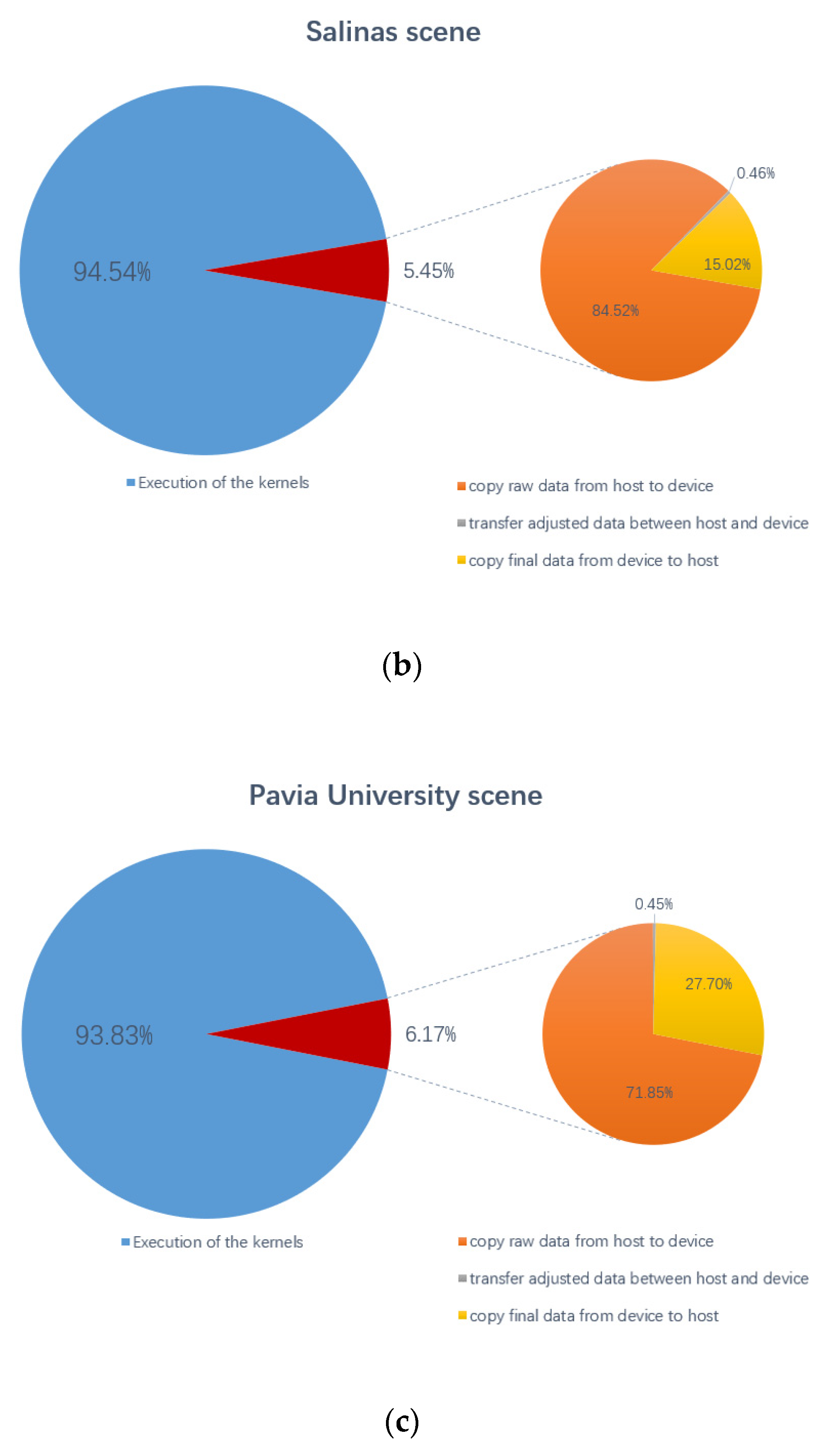
In addition, Figure 8 shows the percentages of data transfer time between the host and the device for the proposed parallel method and gives the percentage of three specific data transmission operations in the total data transfer time. The transfer of adjusted data between the host and the device includes two processes, one is to transfer the results of the second SVD to the host, and the other is to transfer the reshaped data to the device. They are all marked with red lines in Figure 3. It can be observed from the Figure 8 that the data transfer time accounts for a small proportion of the total time of the proposed parallel method, and the maximum is less than 6.5%, which means that the pure calculation time occupies more than 93.5%, which proves the effectiveness of the parallel algorithm, that is algorithm performance depends on processing units themselves (not by data transfers), which is also an important issue for GPU parallelization. At the same time, it can also be obtained that the total time of data transmission is mostly concentrated on the input of the raw data and the output of the final result data. Combined with the results in Table 7, this parallel algorithm has advantages in solving large-scale problems.

5.3. UAV Experiment

The practice is the only standard for testing truth. In order to reflect the practicality of the proposed parallel algorithm, we build a complete set of UAV photoelectric platform. The hardware platform mainly includes four parts: Flight module (UAV), data acquisition module (hyperspectral camera and attitude adjustment frame), ground station module (ground station computer), algorithm execution module (on-board NVIDIA Jetson Xavier). The photoelectric platform and the schematic diagram of the online operation of the entire platform are shown in Figure 9.

The entire UAV flight experiment process is as follows. After the system starts, the ground station computer and the on-board computing device separate independent threads to run their respective communication module parts to maintain wireless communication between the two [37]. Subsequently, the flight controller plans the route and performs hyperspectral imaging according to the predetermined route. At each waypoint, the flight controller informs the data collection module to collect hyperspectral data and hover to stabilize at that waypoint; the data collection module that receives the acquisition command informs the on-board NVIDIA Jetson Xavier after the hyperspectral image is taken, and the on-board computing device runs the specific algorithm and realizes current waypoint to complete the identification effect of the specific target.

The entire calculation process is processed in NVIDIA Jetson Xavier, to ensure that our digital communication module and algorithm execution module are normal and stable, we first simulate it on the ground. NVIDIA Jetson Xavier’s hardware configuration is shown in Table 5. Besides, it has seven working modes at the software level, and the different modes are as shown in

Table 8. Seven working modes of NVIDIA Jetson Xavier.

MODE NAME	MAXN	Mode_ 10w	Mode_ 15w	Mode_ 30w_ all	Mode_ 30w_ 6core	Mode_ 30w_ 4core	Mode_ 30w_ 2core
Power budget	n/a	10w	15w	30w	30w	30w	30w
Number of online CPUs	8	2	4	8	6	4	2
CPU maximum frequency (MHz)	2265.6	1200	1200	1200	1450	1780	2100
GPU maximum frequency (MHz)	1377	520	670	900	900	900	900

.

In order to reflect the performance of the proposed algorithm in different working modes, we select mode_MAXN, mode_10w, and mode_30w_4core. A time test was performed on the three traditional datasets on the ground section. The results are given in Figure 10.

As shown in Figure 10, the computational efficiency of the proposed algorithm is related to the working power. The higher the power, the higher the computational efficiency, and the shorter the time overhead. The parallel algorithm also conforms to the characteristics of the larger spatial dimension and the better the acceleration effect. It is worth mentioning that in the three working modes, the speedup factors are essentially unchanged, which also shows the stability, flexibility, and portability of our parallel implementation.

Therefore, we choose mode_MAXN as the basis for further experiments. Since the official working power of mode_MAXN is not given, we will provide it with a mobile power bank that can output 65 W power according to the rated power of the power adapter, i.e., 65 W. The mobile power bank has a capacity of 30,000 mAh, which can make the NVIDIA Jetson Xavier work for a long time, which is far greater than the time of one flight when the UAV is fully charged.

From the flight controller triggers data acquisition to the classification results return to the ground station, the span is taken as the total time of one shutter process, the predominant time-consuming operations, and their proportion are given in Figure 11 and Figure 12.

As shown in Figure 11 and Figure 12, The data acquisition time is fixed at 5 s and is determined by the camera. After the camera scans (data acquisition), it quickly generates a raw data file in the file system, which is then read by our algorithm as the input. The span of the raw data processing is stable and not time-consuming. Then enter the algorithm execution, as the spatial dimension of hyperspectral data increases, our parallel implementation can always control the algorithm execution within one second and a half, accounting for only about 10% of the total duration, but the OpenCV version of the algorithm process time cost increases rapidly, and takes up about 70% of the total time, which exceeds 40 s. It can be seen that our parallel strategy dramatically reduces the total time, and the total time is dominated by the fixed time of the entire platform, rather than our algorithm itself, which significantly increases the real-time processing capabilities and effects. Considering that the fully loaded safe flight time of the UAV is only 15 min, it has a high practical effect and significance.

Figure 13 shows a schematic diagram of the flight experiment. We fly the UAV to an altitude of 300 m, 38° is the horizontal field angle of the hyperspectral camera (more parameters are shown in Table 3), we shoot at several fixed flight waypoints (only two waypoints are shown in Figure 13), and set the distance between each two flight waypoints to 50 m, which can ensure that each image has enough different fields. Hover the UAV at each waypoint, start camera scans, and generate hyperspectral data for a fixed period of 5 s. After that, the drone can be flown to the next waypoint. Taking into account the acceleration and deceleration process, the stability of the UAV posture, etc., it takes about 10 s to move the UAV to the next waypoint according to our extensive tests. At the same time, the algorithm process, which includes raw data processing, algorithm execution, and classification inference, will be executed during the UAV movement. According to Figure 11 and Figure 12, the algorithm process of our parallel implementation takes about 3.8 s, which means that we can ensure that we have obtained the results data of the previous waypoint at the next waypoint even if considering the data return time, this is of great significance in real-time applications. In other words, we can quickly make judgments and reactions to the following decisions based on the results of the previous waypoint.

We build a scene with several classes to test the classification results of the flight experiment. We customized the jungle tank model, jungle camouflage net, and put them in the real environment. The information of specific classes is given in the form of legends of a specific color in Figure 14.

Figure 14 shows the classification results of aerial scenes of our flight experiment. We only label part of scenes as ground truth and use the entire flight shooting data for prediction. It can be seen that the classification results are very clear, especially the classification of the tank model, the camouflage net, and the environmental background (grass and trees) because they have the same naked eye color—this fully reflects the superiority of the hyperspectral algorithm. What is more worth mentioning is that it only takes a few seconds from camera shooting data to the classification results return to the ground station according to our parallel implementation—this is very important and practical.

6. Conclusions and Future Work

From the perspective of real-time issues, we aim to build software and hardware implementations for parallel processing of hyperspectral images.

Starting from aiming at feature extracting and reducing the noise, an INAPC algorithm for hyperspectral images and its accelerated implementation are introduced. We deploy a complete CPU-GPU collaborative computing solution, and our CUDA implementation is highly encapsulated to facilitate the migration of algorithms to different platforms and environments.

On the other hand, we establish a complete set of UAV photoelectric platform, completed the algorithm migration using the NVIDIA Jetson Xavier, and the flight experiments again verified the effectiveness and practicality of the algorithm. The combination of hardware and software also provides valuable experience and practical significance.

In the future, we would like to add more feature information to the parallel implementation and optimize the noise reduction method, while optimizing the parallel effect, especially optimize the data transmission with more efforts. In addition, the improvement of the entire photoelectric platform needs to consider the coordination of more aspects, such as the protocol of the data interface, the stability of the data transmission, etc.

References

1. Tu, B.; Yang, X.; Li, N.; Zhou, C.; He, D. Hyperspectral anomaly detection via density peak clustering. Pattern Recognit. Lett. 2020, 129, 144–149. [Google Scholar] [CrossRef]
2. Wu, C.; Zhang, L.; Du, B. Kernel Slow Feature Analysis for Scene Change Detection. IEEE Trans. Geosci. Remote Sens. 2017, 55, 2367–2384. [Google Scholar] [CrossRef]
3. Paoletti, M.E.; Haut, J.M.; Fernandez-Beltran, R.; Plaza, J.; Plaza, A.J.; Pla, F. Deep Pyramidal Residual Networks for Spectral-Spatial Hyperspectral Image Classification. IEEE Trans. Geosci. Remote Sens. 2019, 57, 740–754. [Google Scholar] [CrossRef]
4. Zhang, L.; Zhang, L.; Du, B.; You, J.; Tao, D. Hyperspectral image unsupervised classification by robust manifold matrix factorization. Inf. Sci. 2019, 485, 154–169. [Google Scholar] [CrossRef]
5. Peng, J.; Sun, W.; Du, Q. Self-Paced Joint Sparse Representation for the Classification of Hyperspectral Images. IEEE Trans. Geosci. Remote Sens. 2019, 57, 1183–1194. [Google Scholar] [CrossRef]
6. Banerjee, B.P.; Raval, S.; Cullen, P.J. UAV-hyperspectral imaging of spectrally complex environments. Int. J. Remote Sens. 2020, 41, 4136–4159. [Google Scholar] [CrossRef]
7. Lu, J.; Li, W.; Yu, M.; Zhang, X.; Ma, Y.; Su, X.; Yao, X.; Cheng, T.; Zhu, Y.; Cao, W.; et al. Estimation of rice plant potassium accumulation based on non-negative matrix factorization using hyperspectral reflectance. Precis. Agric. 2020. [Google Scholar] [CrossRef]
8. Zhang, X.; Zhao, J.; Yang, G.; Liu, J.; Cao, J.; Li, C.; Zhao, X.; Gai, J. Establishment of Plot-Yield Prediction Models in Soybean Breeding Programs Using UAV-Based Hyperspectral Remote Sensing. Remote Sens. 2019, 11, 2752. [Google Scholar] [CrossRef] [Green Version]
9. Yan, Y.; Deng, L.; Liu, X.; Zhu, L. Application of UAV-Based Multi-angle Hyperspectral Remote Sensing in Fine Vegetation Classification. Remote Sens. 2019, 11, 2753. [Google Scholar] [CrossRef] [Green Version]
10. Zhang, S.; Lu, X.; Nir, G.; Li, Y.; Shao, Y.; Tian, Y.; Fan, L.; Zhang, Y. Estimation of Soil Organic Matter in Coastal Wetlands by SVM and BP Based on Hyperspectral Remote Sensing. Spectrosc. Spectr. Anal. 2020, 40, 556–561. [Google Scholar] [CrossRef]
11. Li, L.; Xie, S.; Ning, J.; Chen, Q.; Zhang, Z. Evaluating green tea quality based on multisensor data fusion combining hyperspectral imaging and olfactory visualization systems. J. Sci. Food Agric. 2019, 99, 1787–1794. [Google Scholar] [CrossRef] [PubMed]
12. Marotz, J.; Kulcke, A.; Siemers, F.; Cruz, D.; Aljowder, A.; Promny, D.; Daeschlein, G.; Wild, T. Extended Perfusion Parameter Estimation from Hyperspectral Imaging Data for Bedside Diagnostic in Medicine. Molecules 2019, 24, 4164. [Google Scholar] [CrossRef] [PubMed] [Green Version]
13. Shimoni, M.; Haelterman, R.; Perneel, C. Hyperspectral Imaging for Military and Security Applications Combining myriad processing and sensing techniques. IEEE Geosci. Remote Sens. Mag. 2019, 7, 101–117. [Google Scholar] [CrossRef]
14. Melgani, F.; Bruzzone, L. Classification of hyperspectral remote sensing images with support vector machines. IEEE Trans. Geosci. Remote Sens. 2004, 42, 1778–1790. [Google Scholar] [CrossRef] [Green Version]
15. Chunhui, Z.; Bing, G.; Lejun, Z.; Xiaoqing, W. Classification of Hyperspectral Imagery based on spectral gradient, SVM and spatial random forest. Infrared Phys. Technol. 2018, 95, 61–69. [Google Scholar] [CrossRef]
16. Paoletti, M.E.; Haut, J.M.; Fernandez-Beltran, R.; Plaza, J.; Plaza, A.; Li, J.; Pla, F. Capsule Networks for Hyperspectral Image Classification. IEEE Trans. Geosci. Remote Sens. 2019, 57, 2145–2160. [Google Scholar] [CrossRef]
17. Jia, X.; Kuo, B.-C.; Crawford, M.M. Feature Mining for Hyperspectral Image Classification. Proc. IEEE 2013, 101, 676–697. [Google Scholar] [CrossRef]
18. Prasad, S.; Bruce, L.M. Limitations of Principal Components Analysis for Hyperspectral Target Recognition. IEEE Geosci. Remote Sens. Lett. 2008, 5, 625–629. [Google Scholar] [CrossRef]
19. Li, W.; Prasad, S.; Fowler, J.E.; Bruce, L.M. Locality-Preserving Dimensionality Reduction and Classification for Hyperspectral Image Analysis. IEEE Trans. Geosci. Remote Sens. 2012, 50, 1185–1198. [Google Scholar] [CrossRef] [Green Version]
20. Villa, A.; Benediktsson, J.A.; Chanussot, J.; Jutten, C. Hyperspectral Image Classification with Independent Component Discriminant Analysis. IEEE Trans. Geosci. Remote Sens. 2011, 49, 4865–4876. [Google Scholar] [CrossRef] [Green Version]
21. Green, A.A.; Berman, M.; Switzer, P.; Craig, M.D. A transformation for ordering multispectral data in terms of image quality with implications for noise removal. IEEE Trans. Geosci. Remote Sens. 1988, 26, 65–74. [Google Scholar] [CrossRef] [Green Version]
22. Li, W.; Zhang, L.; Zhang, L.; Du, B. GPU Parallel Implementation of Isometric Mapping for Hyperspectral Classification. IEEE Geosci. Remote Sens. Lett. 2017, 14, 1532–1536. [Google Scholar] [CrossRef]
23. Torti, E.; Acquistapace, M.; Danese, G.; Leporati, F.; Plaza, A. Real-Time Identification of Hyperspectral Subspaces. IEEE J. Sel. Top. Appl. Earth Obs. Remote Sens. 2014, 7, 2680–2687. [Google Scholar] [CrossRef]
24. Cervero, T.G.; Caba, J.; López, S.; Dondo, J.D.; Sarmiento, R.; Rincón, F.; López, J. A Scalable and Dynamically Reconfigurable FPGA-Based Embedded System for Real-Time Hyperspectral Unmixing. IEEE J. Sel. Top. Appl. Earth Obs. Remote Sens. 2015, 8, 2894–2911. [Google Scholar] [CrossRef]
25. Torti, E.; Danese, G.; Leporati, F.; Plaza, A. A Hybrid CPU–GPU Real-Time Hyperspectral Unmixing Chain. IEEE J. Sel. Top. Appl. Earth Obs. Remote Sens. 2016, 9, 945–951. [Google Scholar] [CrossRef]
26. Lee, J.B.; Woodyatt, A.S.; Berman, M. Enhancement of high spectral resolution remote-sensing data by a noise-adjusted principal components transform. IEEE Trans. Geosci. Remote Sens. 1990, 28, 295–304. [Google Scholar] [CrossRef]
27. Song, M.; Peng, Y.; Jiang, T.; Li, J.; Zhang, S. Accelerated image factorization based on improved NMF algorithm. J. Real-Time Image Proc. 2018, 15, 93–105. [Google Scholar] [CrossRef]
28. Ellenbach, N.; Boulesteix, A.-L.; Bischl, B.; Unger, K.; Hornung, R. Improved Outcome Prediction Across Data Sources Through Robust Parameter Tuning. J. Classif. 2020. [Google Scholar] [CrossRef]
29. Wu, Z.; Shi, L.; Li, J.; Wang, Q.; Sun, L.; Wei, Z.; Plaza, J.; Plaza, A. GPU Parallel Implementation of Spatially Adaptive Hyperspectral Image Classification. IEEE J. Sel. Top. Appl. Earth Obs. Remote Sens. 2018, 11, 1131–1143. [Google Scholar] [CrossRef]
30. Wu, Y.; Gao, L.; Zhang, B.; Zhao, H.; Li, J. Real-time implementation of optimized maximum noise fraction transform for feature extraction of hyperspectral images. JARS 2014, 8, 084797. [Google Scholar] [CrossRef]
31. cuSOLVER. Available online: http://docs.nvidia.com/cuda/cusolver/index.html (accessed on 25 August 2020).
32. Fang, L.; He, N.; Li, S.; Plaza, A.J.; Plaza, J. A New Spatial–Spectral Feature Extraction Method for Hyperspectral Images Using Local Covariance Matrix Representation. IEEE Trans. Geosci. Remote Sens. 2018, 56, 3534–3546. [Google Scholar] [CrossRef]
33. Foody, G.M. Classification accuracy comparison: Hypothesis tests and the use of confidence intervals in evaluations of difference, equivalence and non-inferiority. Remote Sens. Environ. 2009, 113, 1658–1663. [Google Scholar] [CrossRef] [Green Version]
34. Sun, L.; Wu, Z.; Liu, J.; Xiao, L.; Wei, Z. Supervised Spectral–Spatial Hyperspectral Image Classification with Weighted Markov Random Fields. IEEE Trans. Geosci. Remote Sens. 2015, 53, 1490–1503. [Google Scholar] [CrossRef]
35. Li, W.; Chen, C.; Su, H.; Du, Q. Local Binary Patterns and Extreme Learning Machine for Hyperspectral Imagery Classification. IEEE Trans. Geosci. Remote Sens. 2015, 53, 3681–3693. [Google Scholar] [CrossRef]
36. Fang, L.; Li, S.; Duan, W.; Ren, J.; Benediktsson, J.A. Classification of Hyperspectral Images by Exploiting Spectral–Spatial Information of Superpixel via Multiple Kernels. IEEE Trans. Geosci. Remote Sens. 2015, 53, 6663–6674. [Google Scholar] [CrossRef] [Green Version]
37. Zixuan, Z.; Qinhao, W.; Bo, Z.; Xiaodong, Y.; Yuhua, T. UAV flight strategy algorithm based on dynamic programming. J. Syst. Eng. Electron. 2018, 29, 1293–1299. [Google Scholar] [CrossRef] [Green Version]
Figure 1. Compute unified device architecture (CUDA) codes for matrix multiplication.
Applsci 10 06680 g001
Figure 2. Schematic diagram of our threads organization for performing noise estimation.
Applsci 10 06680 g002
Figure 3. Flowchart of the proposed INAPC algorithm parallel implementation.
Applsci 10 06680 g003
Figure 4. Results of the eigenvalue curve of three hyperspectral datasets through choosing rule.
Applsci 10 06680 g004
Figure 5. Effect of using different k in the classification of different datasets. (a) Indian Pines; (b) Salinas scene; (c) Pavia University scene.
Applsci 10 06680 g005
Figure 6. The classification results of ten repeated experiments on the three datasets were obtained by different methods. (a) Indian Pines; (b) Pavia University scene; (c) Salinas scene.
Applsci 10 06680 g006
Figure 7. The false color composite image, the ground truth image, and the INAPC classification map of the three datasets. (a) Indian Pines; (b) Pavia University scene; (c) Salinas scene.
Applsci 10 06680 g007
Figure 8. Percentages of the total GPU time for kernel execution and data transfers. (a) Indian Pines; (b) Salinas scene; (c) Pavia University scene.
Applsci 10 06680 g008aApplsci 10 06680 g008b
Figure 9. (a) The whole photoelectric platform based on UAV; (b) the schematic diagram of the online operation of the entire platform.
Applsci 10 06680 g009
Figure 10. Run times of INAPC for the three datasets at three different working mode on NVIDIA Jetson Xavier.
Applsci 10 06680 g010
Figure 11. Time-consuming of several predominant operations of CUDA and OpenCV version in one shutter process.
Applsci 10 06680 g011
Figure 12. The total time and the proportion of several predominant operations of CUDA and OpenCV version in one shutter process.
Applsci 10 06680 g012
Figure 13. Schematic diagram of the flight experiment.
Applsci 10 06680 g013
Figure 14. Visualized results of our flight experiment. (a) The false color composite image; (b) the ground truth image; (c) the INAPC classification map.
Applsci 10 06680 g014