Featured Application
This work can be applied to turbulence severity estimation in flight, which is fundamental to flight safety of civil aviation aircraft.
Abstract
Atmospheric turbulence is a typical risk that threatens the flight safety of civil aviation aircraft. A method of estimating aircraft’s vertical acceleration in turbulence is proposed. Based on the combination of wing and horizontal tail, the continuous change of aerodynamic force in turbulent flight is obtained by unsteady vortex ring method. Vortex rings are assigned on the mean camber surface to further improve the computing accuracy. The incremental aerodynamic derivatives of lift and pitching moment are developed, which can describe the turbulence effects on aircraft. Furthermore, a new acceleration-based eddy dissipation rate (EDR) algorithm was developed to estimate the turbulence severity. Compared with wind tunnel test data, the aerodynamic performance of the lifting surface was computed accurately. A further test on wing–tail combination showed that the computed pitching moment change due to control-surface deflections approaches the aircraft-modeling data. The continuous change of vertical acceleration at any longitudinal locations of aircraft is obtained in turbulent flight. Compared with traditional transfer function-based EDR algorithms, the proposed algorithm shows higher accuracy and stability. Furthermore, the adverse influence of aircraft maneuvering on EDR estimation is eliminated.
1. Introduction
Atmospheric turbulence—a chaotic motion added to constant wind—is frequently encountered in flight. In particular, the vertical component of turbulence threatens aircraft stability and even flight safety. On one hand, in-flight turbulence reduces passenger riding comfort and even causes causalities. On the other hand, it also leads to the manipulation difficulty for pilots and induces fatigue on aircraft structure [1]. To avoid such hazard, it is therefore fundamental to explore the occurrence mechanism, detection and risk judgment method for turbulence.
Atmospheric turbulence can be categorized into convective turbulence, low-altitude thermals, wake turbulence and clear air turbulence [2]. Clear air turbulence, though seriously threatening the flight safety of civil aviation aircrafts, is difficult for onboard weather radar to observe. A traditional method of assessing the turbulence hazard is by means of pilot weather report (PIREP). A major problem of the subjectively reported PIREP is that the turbulence severity experienced by the reporting aircraft may not be the same experienced by a following aircraft because of the different aircraft type and its configuration [3]. Scholars put forward the method of assessing turbulence severity based on vertical acceleration of aircraft [4]. However, the measured acceleration cannot reflect the turbulence severity because it is in fact the turbulence induced response and is also related to other flight parameters. Based on the measured acceleration value, a further derived equivalent vertical gust velocity (DEVG) method was developed, with airspeed and aircraft mass considered [5]. However, measuring the turbulence via vertical acceleration or DEVG could be sensitive to different aircrafts. We need to obtain an objective evaluation criterion of turbulence severity which is independent of aircraft.
Eddy dissipation rate (EDR), a parameter to determine the amount of energy lost by the viscous forces in turbulence, has been widely used to describe the turbulence severity in recent years [6]. The National Center for Atmospheric Research (NCAR) proposed vertical wind-based and vertical acceleration-based EDR estimation method successively. A major advantage of the vertical wind-based algorithm is that only six parameters are required for computing EDR, including true airspeed, left and right vane angle of attack, inertial vertical speed, pitching and rolling angle [7]. The EDR value is obtained by frequency–domain-based maximum-likelihood estimation. The World Meteorological Organization (WMO) has added turbulence monitoring information in the aircraft meteorological data relay, in which vertical wind-based EDR value is reported [8]. However, this kind of EDR algorithm still must be improved because the air data measurements and derived vertical wind may not be accurate in turbulent flight. Furthermore, considering different aircraft, there are some empirically chosen parameters in the algorithm, including the selection of bandpass frequency and bias-correction term [9].
Vertical acceleration-based EDR algorithms, recovering the turbulence severity from an aircraft’s vertical acceleration response, is a rigorous method with better accuracy theoretically [10]. The acceleration response, initially described by a polynomial fitting function, though lack of adequate accuracy, has been applied in modern EDR estimation [11]. The other way of describing the acceleration response is to build a linear-transfer function from vertical wind to aircraft vertical acceleration. Research shows that vertical turbulence mainly leads to aircraft plunge and pitching motion, inducing aircraft bumpiness. Two linear-transfer functions describing plunge and pitching motion—based on small-perturbation approximations—were built, with vertical turbulence as the only excitation. To eliminate the influence of maneuvering flight and high-frequency structural vibration, a bandpass filter must be cascaded to the transfer function. However, it is still lack of enough accuracy to describe the acceleration response. To further explore the modeling accuracy, four linear-transfer function models reflecting aircraft’s plunge and pitching motion in turbulence were developed, with quasi-static aerodynamic model and controls fixed assumptions [12]. These models were tested, respectively and compared with the recorded acceleration data on Boeing 757 aircraft. In ref [13], real-time turbulent wind effects during aerial refueling were studied. Based on Dryden turbulence model assumption, turbulence parameters were identified. By feeding the identified turbulence into flight dynamics model, the simulation results and recorded data are compared. In ref [14], to study the riding comfort in turbulence, acceleration responses in different seating locations were studied by dynamic simulation. The above studies show that there are major differences between measured and theoretical responses To summarize, the linear-transfer function or fitting function cannot accurately describe the acceleration response of aircraft in turbulence. Since EDR algorithm accuracy can easily be affected by control-surface deflection [15], another significant disadvantage is that with controls fixed assumption and only vertical wind as the excitation, these methods cannot distinguish the acceleration change caused by aircraft maneuvering or turbulence. In order to obtain real turbulence severity in a vertical acceleration-based EDR algorithm, the effect of maneuvering flight on vertical acceleration must be eliminated.
As an effective way of aerodynamic analysis and optimization, vortex lattice method (VLM) can be used to obtain the turbulence-effected vertical acceleration response. In earlier studies, planar VLM was adopted by assigning horseshoe vortices on lifting surface. In recent years, nonplanar vortex lattices are assigned on mean camber surface and vortex rings are formulated to obtain more accurate solutions [16]. Although aerodynamic characteristics can be analyzed accurately by compute fluid dynamics method, VLM is still a popular and rapid medium-accurate computing method. VLM has been widely used in aero–elastic analysis [17], wind turbine design [18], lift and induced drag computation [19], wing design optimization [20] and gust wind response analysis [21]. When it comes to the aero–elasticity and gust wind analysis, the influence of aircraft motion and wake on aerodynamic performance must be considered. Unsteady vortex lattice method (UVLM) is used to solve these problems [17,19,20]. In some special applications, like aerodynamic analysis in aerial refueling formation flight [22,23,24] and innovative flap design [25], VLM possesses the advantage of rapid trial-and-error. NASA has developed wind shear coefficients based on steady VLM [26,27]. With no-sideslip assumption, additional aerodynamic effects induced by shear wind were computed and added to quasi-static aerodynamic model. With the simplified combination of wing and horizontal tail, satisfactory accuracy was obtained by VLM in shear wind. However, steady VLM is not suitable for computing aerodynamic force in high frequency turbulent wind. If the turbulence-effected aerodynamic performance is obtained by unsteady VLM, a more accurate vertical acceleration response can surely be acquired, which will be beneficial to vertical acceleration-based EDR algorithm.
In this study, a method for computing aircraft’s vertical acceleration response in turbulence is proposed. Based on nonplanar and unsteady vortex ring method (VRM), the continuous change of aerodynamic force in turbulent flight will be computed. Furthermore, an acceleration-based EDR algorithm will be developed to estimate the turbulence severity. For a specific wing, the computing results based on VRM will be verified by wind tunnel test data and aircraft-modeling data. After this, aerodynamic force and acceleration changes in turbulent flight will be analyzed. With comparison to theoretical EDR value, the performance of the proposed method will be further analyzed.
2. Vertical Acceleration and Turbulence Severity Estimation
2.1. Unsteady Vortex Ring Method
According to the thin-airfoil theory, the lifting-line method can be used to obtain the lift and induced drag of the straight wing with small sweep angle. The panel method is further applied to the lifting surface with large sweep angle. Different kinds of singularities can be assigned on the panel element and the strength of each singularity is determined according to its boundary condition. After this, the pressure distribution and aerodynamic force are further computed. The most commonly used panel method is VLM, in which horseshoe vortex is selected as the singularity [16]. In turbulent flight, the attitude and aerodynamic angle of civil aviation aircraft can change rapidly, leading to unsteady motion. As a result, the far-field wake is not parallel to the free flow, and conventional VLM with semi-infinite vortex filaments does not have satisfactory accuracy in solving this problem. By superimposing the wake vortices rather than semi-infinite filaments, vortex rings can be used to satisfy the trailing edge conditions. In addition, by assigning the vortex rings on the mean camber surface, the computing accuracy can be effectively improved.
It is the vertical turbulence component which leads to the change of aircraft’s longitudinal response. Aircraft’s vertical acceleration is mainly determined by aerodynamic force change of the wing and horizontal tail. Thus, the aircraft is simplified by wing–tail combination and the vortex rings are distributed on their mean camber surfaces. As shown in Figure 1, vortex rings are assigned on the whole reference area, rather than the lifting surface only exposed outside the fuselage.
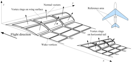
Figure 1.
Vortex rings on mean camber surface of wing–tail combination.
2.2. Grid Generation on Wing-Tail Combination
As shown in Figure 1, the origin point is located on the leading edge of the wing root and a spatial coordinate system is established. A grid with certain number of rows and columns is assigned. The wing and horizontal tail are divided by dozens of rectangular vortex rings. Please refer to Appendix A for grid arrangement and further geometric parameters computation. The wing on one side is divided by rows chord-wise and columns span-wise, and the horizontal tail on one side is divided by chord-wise and span-wise. Since the circulation distribution changes greatly at the wingtip, wing root and leading edge, the neighboring lattices can be redesigned according to the semicircle division method [28]. In addition, the geometric boundary of the control surface is close to the boundary of each vortex ring since elevators and spoilers can be deflected by pilot’s manipulation or automatic flight control system.
As shown in Figure 2a, rectangular vortex rings are arranged on each lattice panel. The leading edge of the vortex ring is located at the 1/4 chord of the grid, the collocation point is located at the midpoint of the 3/4 chord of the grid and the trailing edge is located at the 1/4 chord of the grid in the next row. The trailing edge of the vortex in the last row coincides with the grid boundary. In order to approximate the mean camber surface, the vortex filaments of Section AE and BD are further divided by Section AF and FE, BC and CD, respectively.
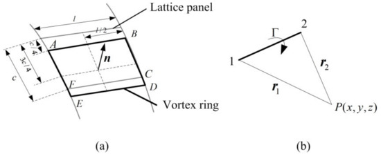
Figure 2.
(a) Vortex ring and (b) induced velocity.
In Figure 2b, according to Biot–Savart law, the velocity induced by a vortex filament at arbitrary point P in space is [16]
In Equation (1), is the induced velocity, is the strength of the vortex filament, is the vector of the vortex filament. and are the position vectors of both ends to an arbitrary point in space. Based on Equation (1), a coefficient vector of induced velocity is defined as
Except for the trailing edge, the induced velocity of a vortex ring to arbitrary point in space can be expressed as the vector sum of the induced velocity by six vortex filaments:
2.3. Vertical Acceleration Computation in Turbulent Flight
2.3.1. Local Velocity Induced by Aircraft’s Unsteady Motion
The nonplanar and unsteady vortex ring method (VRM) is applied to study the aerodynamic characteristics in turbulent flight. Local velocity induced by aircraft’s unsteady motion at arbitrary point can be divided by three parts. The first part is the far-field free flow . The second part is the angular rate effects of the aircraft. The third part is the instantaneous turbulence effects. The local velocity of arbitrary point at any time can be described by Equation (4), with the coordinate of arbitrary point,
2.3.2. Unsteady Aerodynamics in Turbulence
At any collocation point, the boundary condition of zero normal flow through the airfoil’s surface is satisfied, which can be described by Equation (5):
where is the potential function of the flow field. Velocity components at any collocation point are described as .
At any time , as shown in Figure 3, the aircraft moves along the flight path, vortices on the trailing edge fall off at local velocity, generating a series of wake vortices. Local velocity at the trailing edge is defined by
where is the induced velocity of airfoil-attached vortices at trailing edge points m at time . is the induced velocity of wake vortices. The trailing edge continues to move forward with the aircraft and the corner points determined before each time step move forward along the airflow. By determining a new couple of corner points corresponding to the trailing edge points, a new wake vortex ring is constructed. The corner points determined at move forward by . This is repeated at each time step to establish a series of wake vortices. The latest wake vortex ring has the same strength as the trailing edge vortex at . In other word, it is not affected by aerodynamic force. The wake vortices move at local velocity, which is achieved by modifying the positions of the corner point n at each time step:
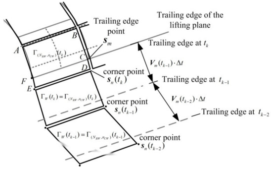
Figure 3.
Nonplanar unsteady vortex ring modeling.
As a result, the induced velocity of wake vortices at collocation points at is obtained. The boundary condition of zero normal flow is adjusted by
By further expanding the above equation, the following linear algebraic equation is obtained:
By solving Equation (9), the circulation of each vortex ring is acquired. It should be noted that there is no vortex ring at . At the first time step , the circulation of each vortex ring is also obtained without wake effects.
Here is an analysis about the boundary condition on each vortex ring. Figure 4a shows the decomposition of boundary condition along the wing chord. In turbulence, the boundary condition at the collocation point is expressed as
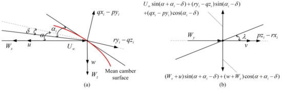
Figure 4.
(a) Boundary condition decomposition along the wing chord and (b) along the wingspan.
As shown in Figure 4b, with the dihedral angle, the boundary condition is further modified by
where stands for the incretion of angle of attack due to control-surface deflection. It can be omitted if there is no deflection. Moreover, shows the camber effects. represents the induced velocity decomposition along each axis.
After obtaining the circulation of each vortex ring, aerodynamic force is further computed according to Kutta–Joukowski theorem [16]. As shown in Figure 5, any vortices and their adjacent vortices need to be superposed on the lattice panel to get actual circulation distribution. Taking the right half wing as an example, the aerodynamic force at the collocation point is
where is air density, is the total induced velocity of airfoil-attached vortex at the collocation point. Since there is no vortex ring in front of the leading edge, equals zero in Equation (12). At the trailing edge, the third item of does not exist because the second half of the vortex ring is not on the panel. At each time step , the aerodynamic force with and without turbulence effects are solved, respectively, which are recorded as and .
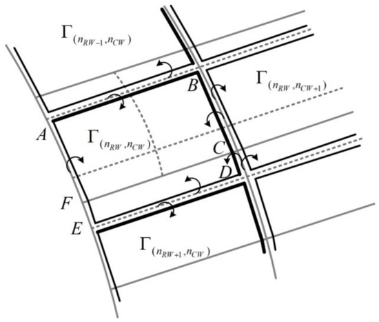
Figure 5.
Neighboring rings for a general vortex ring.
2.3.3. Solution of Vertical Acceleration
Since the lifting surface of the aircraft was simplified to the wing–tail combination, there may exist a gap between computing results and actual aerodynamic force. We try to develop the incremental aerodynamic derivatives induced by turbulence and add them into existing aerodynamic model. The incremental derivatives function as a supplement to the aerodynamic model, rather than replacement. For each collocation point, with the aerodynamic force in turbulence and the force without turbulence effects , the force increment is obtained by . After summing the whole vortex rings, the turbulence-induced incremental aerodynamic force is obtained by
Furthermore, the incremental pitching moment around the gravity center is
The turbulence-effected incremental aerodynamic derivatives are described by Equation (15). Since plunge and pitching motion are the main cause of aircraft bumpiness, the lift incremental derivative and pitching moment incremental derivative are computed by
where is the dynamic pressure, c is the mean chord length. and function as one of the derivative terms in lift and pitching moment coefficients, respectively. Due to the limitation of panel method, the incremental aerodynamic derivatives including side force, rolling and yawing moment cannot be computed accurately. However, it is of less importance to compute lateral motion accurately in the vertical-acceleration estimation. The plunge and pitching motion which mainly lead to aircraft bumpiness can be solved by VRM with a satisfactory precision. Moreover, CFD method can be adopted to obtain more accurate solutions. However, it cannot be solved in real time and needs a complete set of aircraft’s geometric and airfoil parameters. With the nonplanar and unsteady VRM, the real-time change of aerodynamic force caused by turbulence can be acquired accurately. Based on the modified aerodynamic model, flight parameters required in Equation (4) can be obtained by numeric integration [29] or states estimation in flight dynamic model [30]. Here only the differential equation of vertical acceleration and pitching moment are listed:
where and are the pitching and rolling angle at , stands for the inertia matrix. Vertical acceleration at any position on the longitudinal plane is obtained by
where represent the location of gravity center.
2.4. Vertical-Acceleration Based EDR Estimation
The goal of the EDR algorithm, whether based on vertical acceleration or vertical wind, is to recover the same turbulence severity with acceptable accuracy. While the aircraft is flying through turbulence, the intensity and spatial frequency of turbulence are actually obtained by measuring the temporal frequency and acceleration response of aircraft. It is required to recover the objective EDR value which is independent of aircraft’s airspeed, mass and vertical acceleration. As mentioned before, although the wind-based EDR estimation is much easier, there exist deviations in measured air data and empirically selected parameters. In this paper, a new acceleration-based EDR estimation algorithm is proposed.
Given the power spectral density (PSD) of the input vertical turbulence component as and the frequency response function from turbulence input to vertical acceleration , we get the PSD of the acceleration response by
Equation (18) is built up in temporal-frequency domain since the measurements are made by aircraft flying through turbulence with airspeed V. According to Taylor’s frozen-field hypothesis, the length scale of the vertical turbulence component can be obtained by . The estimation is conducted in frequency domain, and the above equation is integrated between the frequency segments and to obtain the acceleration response energy:
For flight conditions of civil aviation aircraft, a bandpass filter should be cascaded to eliminate the influence of aircraft maneuvering and high-frequency structural vibration, where and correspond to the filter’s half-power points. In practice, the lower cutoff frequency must be greater than the phugoid response frequencies, while high-end cutoff frequency is made to lie below the elastic response mode of the given aircraft. For the typical flight conditions of civil aviation aircraft, the frequency band within which most vertical acceleration response occurs corresponds to the inertial sub-range of atmospheric turbulence, and and are chosen as 0.1 and 1.0 Hz, respectively in Equation (19) [10]. The above equation is modified by
To estimate the response energy, the bandpass filter is transformed to time domain first, by Inverse Fourier transform (IFT) as follows:
After this, Parseval’s theorem (assuming local stationary) and the convolution theorem are adopted to yield the approximation [31]:
where is a curve equation obtained by fitting the acceleration calculated by Equation (16). This states that the frequency-limited response mean-square value is obtained by computing a running mean-square value of the bandpass filtered acceleration sequence. Before been discretized, nonzero mean value must be removed in computing the outer integration in Equation (22). The averaging integral 2T () is selected to satisfy the local-stationarity assumption and provide enough data values for statistical stability. The time constant is chosen such that for .
Dryden and von Karman turbulence model are commonly used in describing the stochastic behavior of high-altitude turbulence, while the latter can describe the turbulence characteristics with better accuracy [32]. The energy spectrum of von Karman model is built up according to large amounts of measuring and has a roll-off rate of −5/3 in high frequency section. As an approximation of von Karman model, the roll-off rate of Dryden model is −2 in high frequency section. Since most of the energy responsible for aircraft bumpiness is in the inertial sub-range, EDR estimation is generally based on an underlying turbulence model. In addition, faster-moving aircraft will also be responsive to larger scales that are typically outside the inertial sub-range. Von Karman turbulence model, representing both the inertial sub-range and the larger scales beyond it, has been widely used in both aerodynamics and meteorological field [10]. As a logical choice in describing the turbulence characteristics, von Karman model has been integrated into commonly used EDR estimation algorithm.
In addition, according to the Von Karman and Kolmogorov energy spectrum theory, the PSD of vertical turbulence is approximated by [10]:
The energy spectrum of turbulence depends on the parameter . According to turbulence model, the theoretical EDR value, generally defined as and commonly used to verify the severity estimation algorithm, is obtained. By inserting Equation (23) into Equation (20),
If in Equation (24) is known, the EDR value can be estimated. To estimate the acceleration response, Fourier transform is performed on the vertical acceleration and vertical wind sequence in the period T. After that, the results are converted from time domain to frequency domain to obtain and respectively. The value of forms a new sequence. According to Wiener–Khinchin theorem, the autocorrelation function R of the new sequence by IFT is obtained with as the estimation results. After this, the acceleration response can be acquired. Finally, EDR value is estimated by the following equation:
To summarize, an integrated computation flow for vertical acceleration and turbulence severity estimation is shown in Figure 6. The grid on wing–tail combination is generated beforehand. In the algorithm loop, external turbulence and flight parameters are used to compute local velocity by Equation (4) firstly. After that, the aerodynamic force is computed by nonplanar and unsteady VRM which has been assembled in the dashed box. In each cycle, by toggling the Flag, total aerodynamic force and the force without turbulence effects are computed, respectively to obtain the force increment . Based on the latest incremental derivatives, vertical acceleration is obtained by solving the FDM. Next, the time series of acceleration data are used to estimate by Equation (22). In addition, after fast Fourier transform (FFT), the acceleration series in frequency domain are used to obtain the transfer function together with the frequency–domain vertical turbulence. At the end of each iteration, the estimated EDR value is output by solving Equation (25). It should be noted that the flight parameters including airspeed, attitude and angular velocity can be input by dynamic model integration or by state estimation with airborne measurements.
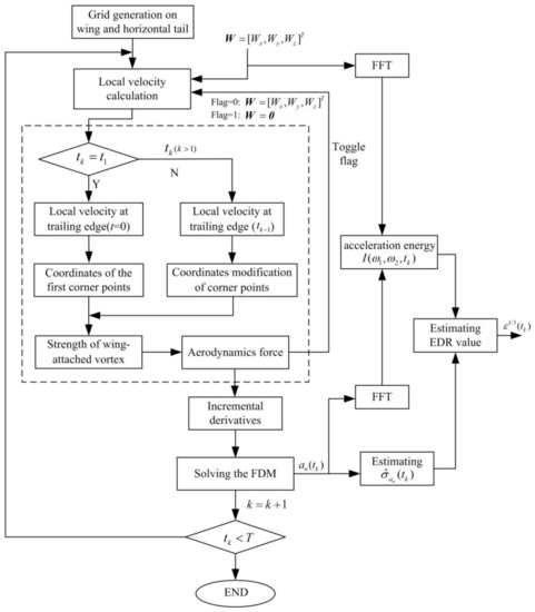
Figure 6.
Computation flow.
3. Experiments and Discussion
In this section, the experimental verification is divided into two parts. First, steady VRM was used to analyze and verify the aerodynamic force of several lifting surfaces in the absence of turbulence. In addition, with the wing–tail combination, the pitching moment change due to control-surface deflection is computed and further compared with aircraft-modeling data. Second—based on nonplanar and unsteady VRM—the changes of aerodynamic force, location of pressure center and incremental aerodynamic derivatives of aircraft in turbulence are explored. After this, four kinds of turbulent wind fields with different intensities are used to analyze the change of acceleration spectra at typical locations of fuselage. Furthermore, the accuracy of the proposed EDR algorithm compared with theoretical EDR value is analyzed. The suppression ability of the new EDR algorithm to maneuvering flight is studied by a climbing-flight simulation.
3.1. Experiments on VRM
3.1.1. Analysis of Grid Convergence
The grid resolution should be first studied to improve the computing efficiency on the premise of ensuring the accuracy. Further experiments are based on the optimized grid level. Here a test was done using geometric and experimental data from NACA Technical Note 1270, in which several NACA-44 series airfoils were tested [33]. The test was to verify the influence of grid resolution on the convergence of aerodynamic coefficients. Based on the NACA-4412 airfoil, four wing geometries were studied, covering low aspect ratio–low sweep angle, low aspect ratio–high sweep angle, high aspect ratio–low sweep angle and high aspect ratio–high sweep angle. Details on the geometries of four test wings are presented in Table 1. Further airfoil parameters are shown in ref [33].

Table 1.
Details of test wings used for grid convergence study.
VRM requires a sufficiently refined grid to achieve results that are grid-independent. Ten different surface grids of increasing mesh density were generated for each of the geometries. Each grid had a constant spacing in both chord-wise and span-wise directions. The lattice number of chord-wise and span-wise are presented in Table 2.
Table 2.
Number of cells included at each grid level used for convergence study.
Vortex rings were all assigned on the mean camber surface. In Figure 7, the changes of the lift coefficient , drag coefficient and pitching moment coefficient about the 1/4 chord point of the root chord are presented, for the four test wings, as a function of the grid refinement level. All the coefficient values were normalized using the value obtained for the finest grid, Grid 10. When it comes to the eighth refinement level, the results for all three aerodynamic coefficients and for all four wing geometries were within 1% of the values obtained with the most refined grid. Thus, satisfactory accuracy can be obtained by adopting Grid 8 configuration.
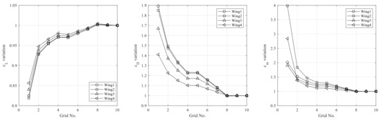
Figure 7.
Convergence of aerodynamic coefficients with grid refinement level.
3.1.2. Computation of Aerodynamic Performance
With the refined grid, the aerodynamic performance of lifting surface computed by nonplanar VRM was compared with wind tunnel test data. The NACA series airfoil data obtained by wind tunnel test are often used as the comparison validation of panel method. The asymmetric NACA-44 series airfoils were chosen for the following experiment. Based on NACA-4424-12 airfoil, a highly swept back, high aspect ratio wing was designed to compare the nonplanar VRM results with wind tunnel test data [33]. Table 3 shows the geometric parameters of the test wing.
Table 3.
Geometric parameters of NACA-4424-12 test wing.
The test airspeed , angle of attack and Reynolds number of . In Figure 8, the changes of , and quarter chord were compared with the wind tunnel test data. It was found that both planar VRM and nonplanar VRM approximate the test data, while nonplanar VRM had higher accuracy. According to ref [33], the aerodynamic characteristics of seven kinds of wings based on NACA-44 series airfoils were further analyzed (Figure 8 shows the first kind of wing). The mean square error (MSE) of both nonplanar and planar VRM was analyzed as shown in Figure 9. The MSE obtained by planar VRM had been reduced to 0.0254, 0.0073 lower than the MSE of planar VRM. It can be concluded that the nonplanar VRM better approximated the wind tunnel test data. If the nonplanar VRM was applied to the analysis of symmetric airfoils, the nonplanar VRM was simplified to traditional planar VRM.
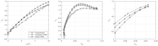
Figure 8.
Comparison of computation and experimental longitudinal aerodynamic coefficients.
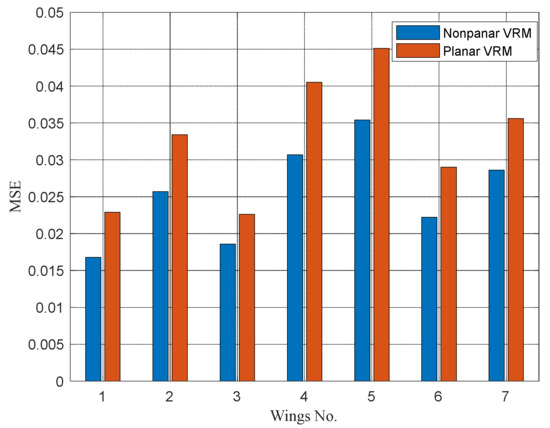
Figure 9.
Mean square error (MSE) of nonplanar and planar vortex ring method (VRM).
3.1.3. Computation of Pitching Moment Coefficient
There exists a gap of longitudinal aerodynamic characteristics between the whole aircraft and the wing–tail combination. Thus, the incremental aerodynamic derivatives and as the supplement to existing aerodynamic model are developed in this paper. However, since the pitching moment change is mainly caused by the deflection of elevator or stabilizer, the computing results based on wing–tail combination should be comparable with authentic aerodynamic data. The modeling data of B737-800 aircraft provides longitudinal pitching moment changes caused by elevator and stabilizer deflections [34,35]. According to the geometric parameters of wing and horizontal tail listed in ref [34], a nonplanar vortex ring model was built. Figure 10 shows the comparison results between computing results and the modeling data in three flight conditions. stands for the pitching moment change due to stabilizer deflection and represents the moment change due to elevator deflection. It should be noted that the flight condition M = 0.76, α = 2°, H = 10,0000 m approximates the cruising flight condition of civil aviation aircraft.
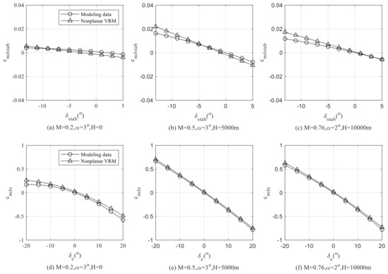
Figure 10.
Comparison of computation and experimental pitching moment coefficients.
Compared with modeling data, the MSE of is 0.0045 and the MSE of is 0.0055. This shows that the pitching moment change caused by the deflection of stabilizer or elevator approximates the modeling data under the above flight conditions. Since the geometric boundary of the control surface approaches the boundary of each vortex ring, VRM can be used to accurately describe the pitching moment change.
The experiments in Section 3.1 prove that the VRM has satisfactory computing accuracy—which provides a good basis for further estimation of aircraft acceleration and turbulence intensity. In particular, the accurate computation of pitching moment coefficient is significant to separate maneuvering flight effects on EDR estimation.
3.2. Experiments on Vertical Acceleration and EDR Estimation
In order to verify the positive effect of the new method on vertical acceleration and turbulence severity estimation, an aircraft flying through turbulence with different intensities was simulated. The time history of vertical acceleration was obtained according to the computation flow shown in Figure 6. Different from Section 3.1, the nonplanar and unsteady VRM was adopted, in which the boundary condition caused by instantaneous turbulence changes in each time step. After the simulation, the estimated EDR value was compared with that of input turbulence.
A 3D turbulence field based on von Karman model was generated according to ref [32]. The wind field generated by time–frequency domain transformation and symmetric expansion conform well to the von Karman turbulence model. Four turbulence cases (TC) were used for experiment. The intensity, vertical scale and input are shown in Table 4. A B737-800 aircraft with was initially trimmed at and , with .
Table 4.
Theoretical input turbulence cases.
The theoretical EDR value is obtained according to ref [10] by:
where and . and represent the intensity and vertical scale of turbulence, respectively. As shown in Figure 6, the generated turbulence components according to von Karman model function as the algorithm input. In addition, the vertical turbulence was also used for computing . After the vertical acceleration was obtained, the response energy was computed. With computed and , the estimated was obtained by Equation (25).
3.2.1. Analysis of Vertical Acceleration Response
A time-history of a control-fixed B737-800 aircraft flying through severe turbulence (TC3) was studied. The vertical acceleration response was obtained according to the computation flow shown in Figure 6, instead of transfer function-based method. As shown in Figure 11, aerodynamic force, pressure center and incremental aerodynamic derivatives changed significantly in turbulence.
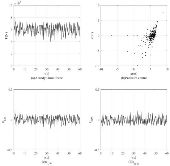
Figure 11.
Time-series of vertical wind and acceleration response.
Under the influence of turbulence, the total aerodynamic force changes between 398~810 kN and the vertical acceleration value changes between 0.66 and 1.35 g. The position of the pressure center, as the acting point of aerodynamic force, changes with the angle of attack. The increment aerodynamic derivative and also change rapidly. According to the small perturbation linearization theory, the transfer function model could only be effective near the equilibrium state. The serious deviation of dynamic model from the equilibrium state brought by the transient turbulence will lead to an increase in the computing error of acceleration response. However, compared with the transfer function-based method, the fluctuation of aerodynamic force was more intense and there were more peak points.
One of the prominent features of the algorithm is that the acceleration on different positions of the fuselage can be obtained. Different locations were identified for investigation. Point A was chosen at the gravity center and point B located at cockpit position, about five meters from point A. Point C located at the aircraft’s tailgate—about 20 m away from the gravity center. The Welch spectral density estimation with the Hamming window function was used [31]. Compared with common spectrum estimation, Welch estimation performs better in frequency resolution and estimation variance [36]. The spectra of acceleration at three locations under TC1–TC4 are shown in Figure 12. For each curve, a 640 s acceleration series was analyzed. This resulted in a total of 10,240 points at a sampling rate of 16 Hz. The length of Hamming window was set as 160; the overlapping rate was selected as 50%.
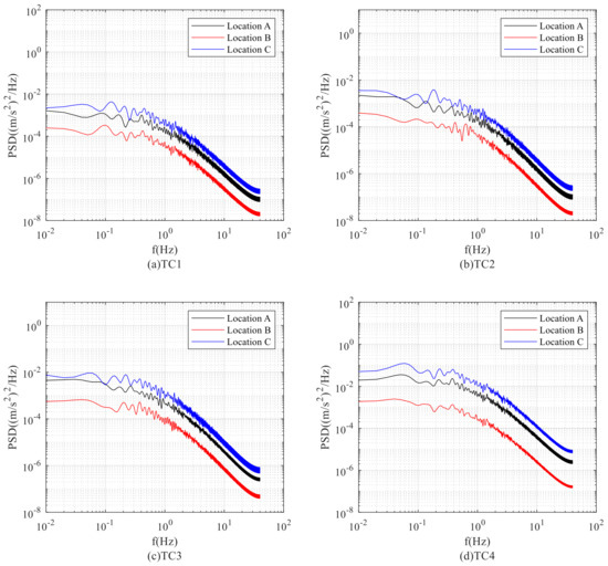
Figure 12.
Acceleration spectrum of different locations.
It was found that the bumpiness at the tail of the fuselage was always stronger than that at the gravity center, while the bumpiness at the nose was the least. This was consistent with the analysis resulted in ref [14]. In moderated turbulence, there was little difference in magnitudes of vertical acceleration between locations A, B and C. However, with the increase of intensity, the difference of acceleration magnitudes increased.
3.2.2. Analysis of EDR Estimation
This section further explores the estimation accuracy by comparing the estimated EDR and input EDR value. Taking the B737-800 aircraft as an example, the EDR values under different intensities were estimated, respectively, and the results were compared with the transfer function-based algorithm. Using the stability derivatives given in the modeling data, a linear-transfer function model similar to the Model 4 in ref [12] was established for comparison, because the Model 4 followed the acceleration transients with the best accuracy [12].
The choice of input-data-length and EDR update was a compromise between having enough resolution to capture instantaneous aircraft bumping and having enough samples in the window to provide stable computational statistics. For aircraft in cruise, a nominal one-minute EDR reporting interval was used. Within the reporting window, sub-windows were chosen for the computation of EDR value. Since a 10 s sub-window was used in EDR estimation, the square root of median values were computed in one-minute period. Here, the estimated EDR values were both generated every 10 s.
Figure 13a shows the 100 times experiment results of the two algorithms. Under the four TCs, the estimated EDR values were all neighboring to the theoretical values. However, with the increase of intensity, the variance of EDR value by transfer function-based method increased, and the number of outliers increased. Figure 13b shows the statistical results of the two algorithms. We found that the performance of the transfer function-based method based on single equilibrium point deteriorated in severe turbulence. The actual flight state seriously deviated from equilibrium point, resulting in increasing deviation in acceleration computation. On the contrary—benefitted from accurately obtained vertical acceleration—the EDR estimation accuracy was still satisfactory. Compared with the transfer function-based method, the variance of EDR value by the recommended method was smaller, and there were few outliers.
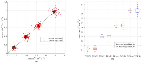
Figure 13.
(a) input and recovered EDR value (b) statistics of two algorithms.
With the Grid 8 refinement, the CPU time of one-time complete EDR estimation was 3.17 s under MATLAB 2018a software environment with i7-9700 processor. The CPU time of vertical acceleration computation was 2.79 s, which mainly contributed to the algorithm complexity. As a result, the algorithm was capable to output the EDR value every 10 s. If the code was converted to C/C++, it could be further optimized and embedded into a real-time system onboard the aircraft. Furthermore, it should be noted that real atmospheric turbulence conforms to von Karman model in a probabilistic sense. The proposed EDR estimation algorithm was still effective by real input of turbulence measurements.
A major problem of the commonly used EDR algorithm is that the control-surface deflection has adverse effects on EDR estimation [15]. As far as the traditional acceleration-based EDR algorithm is concerned, there is no control input in transfer function. With the recommended method in this paper, the vertical acceleration induced by aircraft control or vertical turbulence can be effectively distinguished. The effect of turbulent wind on the vertical acceleration is effectively separated from the aerodynamic force . Therefore, the change of incremental aerodynamic derivatives is only decided by turbulent wind.
A simulation was designed in which the aircraft was approved to climb to the altitude above 11,000 m after encountering turbulence. As shown in Figure 14, during this process, the elevator deflected, and the aircraft kept climbing at a pitch angle of 5 degrees. In order to explore the dynamic process of EDR estimation, the EDR value was given per second in a sliding window of 10 s. The change of aerodynamic force and vertical acceleration caused by turbulence and elevator deflection were obtained. Through the computation of incremental derivatives, the influence of elevator-induced maneuvering was eliminated. Therefore, this new method only improved the accuracy of acceleration response calculation, but also effectively separated the adverse effects of aircraft maneuvering flight on EDR estimation.
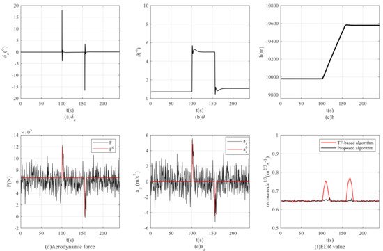
Figure 14.
Eddy dissipation rate (EDR) calculation under elevator deflection.
4. Conclusions
The accurate estimation of turbulence severity is important to flight safety of civil aviation aircraft. This paper proposes a new method for aircraft vertical acceleration and EDR estimation. Some innovations are as follows:
- (1)
- Based on the combination of wing and horizontal tail, an unsteady vortex ring method was introduced to compute the aerodynamic force induced by turbulence. In addition, three innovative operations were proposed to improve the calculation accuracy. First, vortex rings were distributed on the mean camber surface. Second, the semicircle division method was adopted to refine the lattices neighboring to wingtip, wing root and leading edge. Third, the divided lattices were as close as possible to the structural boundary of the control surface. Through the comparison of wind tunnel test data and aircraft-modeling data, we showed that with the proposed method, the aerodynamic force of the lifting surface was computed with high accuracy. The pitching moment change of real commercial aircraft was obtained accurately by the wing–tail combination.
- (2)
- An integrated computation flow for estimating vertical acceleration and turbulence severity was proposed. The fluctuation of vertical acceleration at arbitrary longitudinal locations of aircraft was computed. By the separation of turbulence-induced and maneuvering-induced aerodynamic force, lift and pitching incremental aerodynamic derivatives were developed. Compared with traditional transfer function-based algorithm, the new acceleration-based EDR algorithm showed higher accuracy and stability. In addition, the adverse influence of aircraft maneuvering on EDR estimation could be effectively eliminated.
This paper is the first attempt to apply the unsteady panel method on the estimation of vertical acceleration and turbulence severity, and some preliminary conclusions are obtained. In the future, the vortex ring model and related algorithm will be refined to further improve the accuracy of acceleration and EDR estimation.
Author Contributions
Conceptualization, Z.G.; methodology, Z.G. and D.W.; software, Z.G. and D.W.; validation, D.W. and Z.X.; formal analysis, Z.X.; investigation, Z.G.; resources, Z.G.; data curation, Z.G.; writing—original draft preparation, Z.G.; writing—review and editing, Z.G. and Z.X.; visualization, Z.X.; supervision, Z.G.; project administration, Z.G.; funding acquisition, Z.G. All authors have read and agreed to the published version of the manuscript.
Funding
This research was funded by Natural Science Foundation of China, Grant Number [NSFC: U1733122, U1533120].
Conflicts of Interest
The authors declare no conflict of interest.
Appendix A
This appendix shows the method of grid arrangement and further geometric parameter computations. Wing and horizontal tail on the right side are taken as an example as shown in Figure A1.

Figure A1.
Grid distribution on wing and horizontal tail.
Figure A1.
Grid distribution on wing and horizontal tail.

The ith grid number is defined as
In Figure A1, for
and row, and represent the interception point on the root chord and tip chord, respectively. is the span length of the and grid boundary. The specific coordinate is described as.
As a result, the coordinate of the starting point of the grid which locates in row and column is
. The coordinate of the end point of the grid is .
Accordingly, the coordinate position of corresponded grid on horizontal tail is calculated as follows
As a result, the coordinate of the starting point of the grid which locates in row and column is . The coordinate of the end point of the grid is .
References
- Gao, Z.X.; Fu, J. Research on robust LPV modeling and control of aircraft flying through wind disturbance. Chin. J. Aeronaut. 2019, 32, 1588–1602. [Google Scholar] [CrossRef]
- Schaffarczyk, A.P. Measurements of high-frequency atmospheric turbulence and its impact on the boundary layer of wind turbine blades. Appl. Sci. 2018, 8, 1417. [Google Scholar] [CrossRef]
- Boeing Jeppesen Company. JetPlan User’s Manual; Boeing Jeppesen Company: Englewood, CO, USA, 2014. [Google Scholar]
- Ellrod, G.; Knapp, D. An Objective Clear-Air Turbulence Forecasting Technique: Verification and Operational Use. Weather Forecast. 1992, 7, 150–165. [Google Scholar] [CrossRef]
- Wu, Y.; Zhou, L.; Liu, K.; Huang, C.; Shu, Z. AMDAR based statistical analysis on the features of cross-ocean airplane turbulence over china’s surrounding sea areas. J. Meteorol. Sci 2014, 34, 17–24. [Google Scholar]
- Kim, S.H.; Chun, H.Y.; Chan, P.W. Comparison of turbulence indicators obtained from in situ flight data. J. Appl. Meteorol. Climatol. 2017, 56, 1609–1623. [Google Scholar] [CrossRef]
- Cornman, L.B.; Meymaris, G.; Limber, M. An update on the FAA aviation weather research program’s in situ turbulence measurement and reporting system. In Proceedings of the 11th Conference on Aviation, Range, and Aerospace Meteorology, Hyannis, MA, USA, 4–8 October 2004. [Google Scholar]
- WMO. Aircraft Meteorological Data Relay (AMDAR) Reference Manual; World Meteorological Organization: Geneva, Switzerland, 2003. [Google Scholar]
- Sharman, R.D.; Corman, L.B.; Meymaris, G. Description and derived climatologies of automated in situ eddy-dissipation rate reports of atmospheric turbulence. J. Appl. Meteorol. Climatol. 2014, 53, 1416–1432. [Google Scholar] [CrossRef]
- Larry, B.C.; Corinne, S.M.; Gary, C. Real-time estimation of atmospheric turbulence severtity from in-situ aircraft measurements. J. Aircr. 1995, 32, 171–177. [Google Scholar]
- Huang, R.S.; Sun, H.B.; Wu, C. Estimating eddy dissipation rate with QAR flight big data. Appl. Sci. 2019, 9, 5192. [Google Scholar] [CrossRef]
- Billy, K.B.; Brett, A.N. Aircraft Acceleration prediction due to atmospheric disturbances with flight data validation. J. Aircr. 2006, 43, 72–81. [Google Scholar]
- Atilla, D.; Timothy, A.L. Flight data analysis and simulation of wind effects during aerial refueling. J. Aircr. 2008, 45, 2036–2048. [Google Scholar]
- Nicholas, B.; Christiaan, R. Tentative study of passenger comfort during formation flight within atmospheric turbulence. J. Aircr. 2013, 50, 886–900. [Google Scholar]
- Paul, A.R.; Bill, K.B.; Roland, L.B. Optimization of the NCAR in situ turbulence measurement algorithm. In Proceedings of the 38th Aerospace Sciences Meeting and Exhibit, Reno, NV, USA, 10–13 January 2000; AIAA: Reston, VA, USA. [Google Scholar]
- Katz, J.; Plotkin, A. Low Speed Aerodynamics, 2nd ed.; Cambridge University Press: Cambridge, UK, 2001. [Google Scholar]
- Joseba, M.; Rafael, P.J.; Michael, R. Graham. Applications of the unsteady vortex-lattice method in aircraft aeroelasticity and flight dynamics. Prog. Aerosp. Sci. 2012, 55, 46–72. [Google Scholar]
- Xu, B.; Wang, T.G.; Yuan, Y.; Zhao, Z.Z.; Liu, Z.M. A Simplified Free Vortex Wake Model of Wind Turbines for Axial Steady Conditions. Appl. Sci. 2018, 8, 866. [Google Scholar] [CrossRef]
- Robert, J.S.S.; Rafael, P.; Joseba, M. Induced-drag calculations in the unsteady vortex lattice method. AIAA J. 2013, 51, 1775–1779. [Google Scholar]
- Oliviu, S.G.; Andreea, K.; Ruxandra, M.B. A new non-linear vortex lattice method: Applications to wing aerodynamic optimizations. Chin. J. Aeronaut. 2016, 29, 1178–1195. [Google Scholar]
- Liu, Y.; Xie, C.C.; Yang, C.; Cheng, J. Gust response analysis and wind tunnel test for a high-aspect ratio wing. Chin. J. Aeronaut. 2016, 29, 91–103. [Google Scholar] [CrossRef]
- Luke, H.P.; Ruben, E.P.; Peter, W.J. Wake modelling for aerial refueling using aerodynamic adjoints. In Proceedings of the 2018 AIAA Atmospheric Flight Mechanics Conference, Kissimmee, FL, USA, 8–12 January 2018; AIAA: Reston, VA, USA. [Google Scholar]
- Luke, H.P.; Ruben, E.P.; Peter, W.J. Wake modelling with embedded lateral and directional stability sensitivity analysis for aerial refuelling or formation flight. In Proceedings of the AIAA Scitech 2019 Forum, San Diego, CA, USA, 7–11 January 2019; AIAA: Reston, VA, USA. [Google Scholar]
- Jan, L.; Alexander, M.; Eike, S. Flight dynamics of CS-25 aircraft in formation flight with atmospheric disturbances. In Proceedings of the 2018 AIAA Aerospace Sciences Meeting, Kissimmee, FL, USA, 8–12 January 2018; AIAA: Reston, VA, USA. [Google Scholar]
- Ezra, T.; Nhan, N. Unsteady aeroservoelastic modeling of flexible wing generic transport aircraft with variable camber continuous trailing edge flap. In Proceedings of the AIAA Aviation: 33rd AIAA Applied Aerodynamics Conference, Dallas, TX, USA, 22–26 June 2015; AIAA: Reston, VA, USA. [Google Scholar]
- Dan, D.V.; Roland, L.B. Effect of spatial wind gradients on airplane aerodynamics. J. Aircr. 1989, 26, 523–530. [Google Scholar]
- Daniel, C.; Gustavo, E.C.F.; Eric, T. Transonic and viscous models for vortex lattice method applied to transport aircraft. In Proceedings of the 35th AIAA Applied Aerodynamics Conference, Denver, CO, USA, 5–9 June 2017; AIAA: Reston, VA, USA. [Google Scholar]
- Brenden, P.E.; David, S.G. A quasi-continuous vortex lattice method for unsteady aerodynamics analysis. In Proceedings of the AIAA Aerospace Sciences Meeting, Kissimmee, FL, USA, 8–12 January 2018; AIAA: Reston, VA, USA. [Google Scholar]
- Stevens, B.L. Aircraft Control and Simulation, 3rd ed.; Wiley: New York, VY, USA, 2015. [Google Scholar]
- Jategaonkar, R.V. Flight Vehicle System Identification: A Time Domain Methodology, 2nd ed.; Progress in 199Astronautics and Aeronautics; AIAA: Reston, VA, USA, 2015. [Google Scholar]
- Stoica, P.; Moses, R. Spectral Analysis of Signals; Pearson Education: Upper Saddle River, NJ, USA, 2005. [Google Scholar]
- Gao, Z.X.; Gu, H.B. Generation and application of spatial atmospheric turbulence field in flight simulation. Chin. J. Aeronaut. 2009, 22, 9–17. [Google Scholar]
- Robert, H.N.; Thomas, V.B.; Gertrude, C.W. Experimental and Calculated Characteristics of Several NACA 44-Series Wings with Aspect Ratios of 8, 10, and 12 and Taper Ratios of 2.5 and 3.5; NACA TN-1270; National Aeronautics and Space Administration: Washington DC, USA, 1947. [Google Scholar]
- Boeing Company. Aerodynamic Data and Flight Control System Description for the 737-600/-700/-800/-900 Training Simulator; D611A001-vol1, rev H; Boeing Company: Chicago, IL, USA, 2003. [Google Scholar]
- Boeing Company. Aerodynamic Data and Flight Control System Description for the 737-600/-700/-800/-900 Training Simulator; D611A001-vol3, rev H; Boeing Company: Chicago, IL, USA, 2003. [Google Scholar]
- Lichota, P.; Tischler, M.B.; Szulczyk, J.; Berger, T. Frequency Responses Identification from Multi-axis Multisine Manoeuvre. In Proceedings of the AIAA Scitech 2019 Forum, San Diego, CA, USA, 7–11 January 2019; AIAA: Reston, VA, USA. [Google Scholar]


© 2020 by the authors. Licensee MDPI, Basel, Switzerland. This article is an open access article distributed under the terms and conditions of the Creative Commons Attribution (CC BY) license (http://creativecommons.org/licenses/by/4.0/).