Abstract
Safety is a major concern for autonomous vehicle driving. The autonomous vehicles relying solely on ego-vehicle sensors have limitations in dealing with collisions. The risk can be reduced by communicating with other vehicles sharing sensed information. In this paper, we study a real-time multisource data fusion scheme based on Dempster–Shafer theory of evidence (DS) through cooperative vehicle-to-vehicle (V2V) communications. The classical DS can produce erroneous outputs when confidences are highly conflicting. In particular, a false negative error on object detection may lead to serious accidents. We propose a novel metric to measure distance between confidences on the collected data taking the asymmetry in the importance of sensed events into account. Based on the proposed distance, we consider the weighted DS combination in order to fuse multiple confidences. The proposed scheme is simple, and enables the vehicles to combine confidences in real-time. From real-world experiments, we show that it is feasible to lower the false negative rate by the proposed data fusion scheme, and to avoid accidents using the proposed collision warning system.
1. Introduction
Autonomous vehicles have been considered as a key technology for intelligent transportation systems. According to the research by National Highway Traffic Safety Administration (NHTSA) in 2015, human error causes around 94% traffic crashes [1], and autonomous vehicles are expected to reduce traffic crashes drastically by minimizing drivers’ mistakes [2]. The design of operating software as well as diagnostics tool for autonomous driving have been actively investigated [3]. In particular, a proper anti-collision system is one of the most crucial components of autonomous vehicle systems.
The information including location, distance between adjacent vehicles, and the vehicle velocity can be obtained by the equipped sensors such as radar, Global Positioning System (GPS), and cameras. Collision avoidance systems based on sensing data are actively studied [4,5], including systems to fuse the sensing data obtained from multiple sensors, e.g., combining data from radar and cameras [6]. However, autonomous vehicle systems relying solely on ego-vehicle sensors have limitations in dealing with the collisions due to reasons such as bad weather, sensor malfunctioning, or blind spots, etc. [7,8,9]. The risk can be reduced by utilizing sensed information from the neighboring vehicles through Vehicle-to-Vehicle (V2V) communication [10,11] such as Dedicated Short Range Communications (DSRC) [12] which can support safety applications in high data rates [13,14].
In order to leverage sensed data from multiple vehicles in real-time, we require a data fusion system with low complexity and high reliability. In multisensor systems, there is uncertainty caused by inaccuracy of sensors or complicated sensing environment [15]. In this respect, the “Dempster–Shafer theory of evidence (DS)” [16,17] is a widely used evidence theory to comprehensively fuse multisource information including uncertainty. It does not require any priori information and requires a simple calculation where the outcome can be reinforced as more data become available [18,19,20].
Although DS has many advantages, the classical DS combination may yield unreasonable outputs when evidences are highly conflicting [18,19,20]. This is critical for autonomous vehicle safety, i.e., vehicles may have erroneous sensing results. Data fusion can cause either false positive or false negative errors. The former is a false alarm, i.e., the vehicle falsely identifies a nonexisting object as an existing one. The latter represents misdetection of an existing object or obstacles. In the context of autonomous vehicle safety, false negatives are significantly dangerous [21] according to the case studies on autonomous vehicle accidents [22]. Therefore, we would like to put more emphasis on the confidence in existence rather than nonexistence of objects, and this necessity results in an asymmetry in the importance of sensed events. However, most of existing works do not consider this aspect. Although there are many works which incorporate the degree of conflict into a fusion method [23,24,25,26,27], the studies on evidence distance taking the aforementioned issue into account are rare. In this paper, we develop a novel metric for evidence distance to measure conflict by assigning asymmetric weights to sensed results and propose a real-time data fusion scheme based on the new metric. In addition, we outline a V2V communication method for anti-collision systems in which the proposed data fusion scheme can be effectively applied.
We summarize the main contributions of this paper as follows.
- (1)
- A new metric for evidence distance for real-time data fusion. We propose a novel metric for autonomous vehicle to measure distance between confidences on detected events of asymmetric importance. Next, we propose real-time data fusion scheme based on the new distance, which combines multiple sensing data from adjacent vehicles. We show that the proposed scheme has low complexity, and one can obtain consistent output irrespective of the order of the data to be combined, which is beneficial in the autonomous vehicle environment. In other words, the method is insensitive to external factors that may affect data arrival time such as channel states or vehicle speed.
- (2)
- An integrated collision warning protocol for autonomous vehicles. We propose a cooperative collision warning protocol integrating the proposed data fusion scheme. For real-time operation, the system is composed of technologies in various fields that can guarantee low latency and high reliability. By experiments, we show that the method takes only a few milliseconds to return credible detection of nearby objects.
- (3)
- Experiments with real-world data. By simulation, we show that the proposed scheme reduces false negative errors as compared to the existing methods. In addition, we conduct real-world experiments and show that the proposed system not only prevents collision from blind spots, but also compensates for inaccurate sensing information.
A comprehensive evaluation of the proposed data fusion shows that our scheme reduces fault diagnosis compared to the baseline methods. In addition, the proposed scheme has low complexity, which enables combining gathered data in real-time. Next, experiment results reveal that the proposed collision warning system with data fusion can successfully detect and avoid imminent collisions.
The rest of this paper is organized as follows. In Section 2, we present related works. In Section 3, we introduce background evidence theory and propose the data fusion schemes based on a new metric for evidence distance. The collision warning system that involves the proposed data fusion processes is proposed in Section 4. Section 5 shows the performance evaluation and experiment results with real-world data, and Section 6 concludes this paper.
2. Related Work
There have been several works which implement DS-based multisource data fusion for autonomous vehicle safety. In [28], a method for calculating the probabilities of existence of nearby objects was proposed. From the local sensing results at ego-vehicle, the existence probability is obtained by the DS fusion. A trajectory selection problem was considered in [29], which proposed a decision-making algorithm based on multicriteria such as safety, comfort, and energy consumption. The DS is used for risk assessment, which combines multiple local risk levels obtained from the predefined multiple criteria. However, as their schemes rely only on ego-vehicle’s information, it has limitations on collisions predictions. In [30,31], collision avoidance schemes based on occupancy grid for autonomous vehicle were considered. The state of cells in occupancy grid is determined by the DS that combines the Light Detection And Ranging (LiDAR) data. In [32], the authors proposed a real-time object detection algorithm. The DS is used to fuse the features extracted from sparse point clouds, and experimental results showed good efficiency in the urban traffic environments. However, most of these works focus on the classical DS combination scheme, which may result in erroneous output when the input confidences are highly conflicting.
To overcome the shortcoming of classical DS dealing with conflicting confidences, several distance metrics for evidence and improved DS fusion schemes were proposed. The metric called the Jaccard index, which is based on the cardinalities of the union and intersection of two subsets, is widely used [24]. In [27], a new distance measure which is more sensitive to change of evidence was presented. A pignistic probability transformation based distance measures were studied in [33,34]. Despite many attempts, distance metrics accounting for the asymmetry in the importance of sensed events were not fully studied. To incorporate new distance metrics in DS, modified DS fusion methods were proposed. In [25], a new weighted DS combination scheme was proposed where weights are calculated by distance measure. Moreover, in order to manage confidence conflicting, weighted combination schemes based on conventional distance with uncertainty [26] or ambiguity measures [35,36] were also proposed. However, the above state-of-the-art DS fusion schemes use a distance metric which assumes the evidences are of equal importance. Therefore, it is difficult to apply those fusion methods directly to the autonomous vehicle environment in which the evidences and related events potentially differ in their importance.
In [37], collision avoidance at intersections was studied with real-world experiments. V2V communication is used to share each vehicle’s information such as velocity, and then vehicle trajectories are estimated by Kalman filter. Based on trajectory estimation, each vehicle controls its velocity to avoid collision. In [38], a system for cooperative collision avoidance for overtaking scenario was proposed. For forward (rear-end) collision avoidance, the work in [5] uses deep learning, and the authors of [39] presented a collision avoidance scheme considering the measurement uncertainty in sensors. Although there exist many studies on collision prediction and avoidance, in-depth studies on data fusion for cooperative sensing in autonomous vehicles are necessary.
3. Proposed Real-Time Data Fusion Method Based on a New Distance Metric
Autonomous vehicles can exchange sensing data acquired from various sensors through V2V communication. In order to leverage sensing data from multiple sources in real-time, we require a data fusion system with low complexity and high reliability. In this section, we introduce an inter-vehicle data fusion method for identifying nearby objects.
We classify the type of sensing data into two categories: “object” and “trajectory”. The former is associated with the existence of an object and, given that the object exists, the class of the object. The latter is related with trajectory of an object such as position and velocity. According to these data types, we will adopt different data fusion schemes. We first discuss data fusion associated with “object” type data.
3.1. Data Fusion for Object Information
3.1.1. Dempster–Shafer Theory of Evidence
In general, with more data available, higher credibility in the prediction can be achieved. At the same time, under the autonomous vehicle environment, the decision should be made in real-time. In a multisensor environment, there exists uncertainty due to limited accuracy of sensor measurements or complicated sensing environment [15]. To address these issues, we adopt Dempster–Shafer theory of evidence, in short DS [17], as a tool for combining gathered data in order to improve detection accuracy by reinforcing the output based on the sensed data from peer vehicles. Misdetection of objects due to erroneous sensing can be avoided by fusing the data obtained from peers. Moreover, DS is effective in managing uncertainty in multisensor environments [15]. We begin by summarizing the mathematical framework of DS [16,19,20,40,41].
In DS, the frame of discernment [17] is the set of all possible mutually exclusive and complete states of system denoted by . A Basic Probability Assignment (BPA) function is a mass function which assigns confidence in each subset of , i.e., . The BPA function satisfies the following conditions,
In this paper, we will use term of confidences to indicate BPAs. The elements of the power set having a non-zero mass are called focal elements.
We combine multiple confidences into a single output using the DS rule of combination. Let us consider two confidences, and , which believe X is true. The DS fuses these confidences [17], denoted by , as follows,
We determine the existence and class of an object by two consecutive stages of DS. Prior to classifying objects, we identify whether a detected object indeed exists or not, i.e., an inaccurate sensor can report that an object is detected even if there is nothing, and vice versa. Thus, we first identify the existence, and, if the existence of an object positively identified, second determine the class of the object. The process of the object information data fusion is depicted in Figure 1.
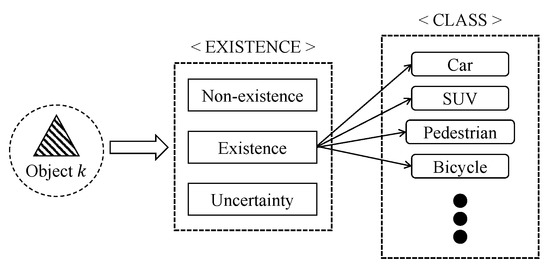
Figure 1.
Determining the object type information.
3.1.2. Data Fusion for the Existence of Objects
For the problem of determining existence, the frame of discernment is given by . In this paper, we use notation to represent the powerset of , i.e., {existence}, {non-existence}, {uncertainty (=existence or non-existence)}} where the elements are denoted by E, N, and U, respectively. Let us define as the confidence at vehicle i about object k that is committed to , and is defined to be the set of confidences. For two vehicles i and j, we can calculate for each element from (3) as follows,
where . For instance, given and , is given by .
Below we define U or the “uncertainty” element, in a rigorous manner. There are two types of uncertainty. The first type is the uncertainty due to inherent limitation of a sensor. For example, a vision sensor cannot detect objects behind obstacles. As shown in Figure 2, the vehicle cannot recognize the existence of the completely occluded object unless a peer vehicle reports the object to that vehicle even if the object is within the sensing area. In this case, the confidence assignments by vehicle i about k is given by
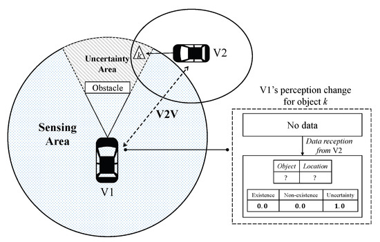
Figure 2.
Definitions of sensing and uncertainty areas. The object in uncertainty area can be perceived through V2V communication.
The second type of uncertainty is from the limited accuracy of sensors. The accuracy of a sensor may be known in advance from its manufacturer [42]. In addition, the confidence can be adjusted for the environment such as weather condition or the distance to the object [16]. For example, we can set the BPAs for clear and rainy days to and , respectively, where is a system parameter.
However, the classical DS combination may yield unreasonable outputs when evidences are highly conflicting. This problem is due to combining in (3) which ignores the conflicts in evidence. In order to illustrate this problem, let us consider the following example [19,40,43]. Given 3 events and 2 Observers, Observer 1 and 2 assign and as confidences in Z, respectively. Although Observers are quite certain that either event A or C has occurred, the combination assigns the highest confidence to event B as . Therefore, in order to deal with highly conflicting evidences, we consider the evidence of distance in order to measure the degree of conflict among evidences [24,33].
3.1.3. Proposed Metric for Evidence Distance
Based on the confidence assignment, in Jousseleme’s approach [24], the similarity between two subsets is measured by their cardinality using the Jaccard index, , and the distance increases with the degree of conflict between two sets of confidences. Specifically, given two confidences and on the same frame of discernment , the Jousselme distance between them is defined as follows [24],
where and are vectors associated with and , respectively, and P is matrix whose elements are defined by
The underlying premise of this approach is that elements of the frame of discernment are equally important. However, in navigational safety, false negative is significantly dangerous [44,45]. That is, the sensor did not report the existence of an object although the object existed. Therefore, we would like to put more emphasis on the confidence of E than the other elements. This results in an asymmetrical importance among the elements in the frame of discernment. In this paper, we propose a novel distance metric to measure conflict by applying asymmetric weights to each element in the frame of discernment, and the weighted DS combination [15,25,26,35] is considered to fuse the confidences according to the proposed conflict distance.
Definition 1.
For the proposed distance metric, we define the weighted cardinality for as follows,
where is a weight function .
Through , we can flexibly adjust the weights depending on the importance of the associated elements, i.e., a larger weight indicates a higher importance. By doing so, we can put asymmetric emphasis on the elements in the frame of discernment. Our approach generalizes the similarity measure used by the existing methods in which the volume of similarity is determined by the number of elements in subsets having identical weight [24,27]. We compute the weighted similarity matrix Q as follows,
For , given the confidences of vehicle i and j about object k, the distance between them is defined by
where is vector of . We show that the proposed distance in (10) satisfies all four conditions on distance metrics, which are non-negativity, nondegeneracy, symmetry, and triangle inequality [24].
Proposition 1.
The proposed distance is a distance metric on .
Proof of Proposition 1.
For , we have 3 elements given by . Let us denote the weighted cardinalities corresponding to each element as , , and , respectively, i.e., . We can compute the weighted similarity matrix Q by (9), and suppose that the matrix Q is partitioned into the form such that
Let be the Schur complement of A in Q, which is defined by . Then, Q is positive definite if and only if the following properties hold,
is satisfied by property of identity matrix A. can be expressed as
The relation (13) can be derived by Definition 1 in (8) and . Inequality (14) holds due to , and . Thus, (10) is an induced norm [24,46], which implies that it satisfies all of four conditions on the metric distance. □
We illustrate an example of the proposed distance metric in Figure 3. In both cases, Observers 1 and 2 have the same Jousselme distance given by 0.7649 due to the symmetry of confidences of E and N. In our approach, given the weights as , , and , we obtain new distance for each case as 0.7147 and 0.8124, respectively. The result can be explained as follows. We assign high importance to “existence” by . For the case of and , the level of conflict between confidences is high, but Observer 1 is highly confident of existence, i.e., . In this case, it is regarded that two confidence vectors have a shorter distance than that by the conventional metric. Contrary to this, Observer 1 in case 2 has relatively low confidence in existence than case 1, i.e., . In spite of the same degree of conflict, by putting more emphasis on E, the dissimilarity between the confidences become greater. Therefore, we obtain the distance in case 2 given by , which will affect the result of data fusion. Next, we explain how the existence of the object is determined based on the proposed distance.
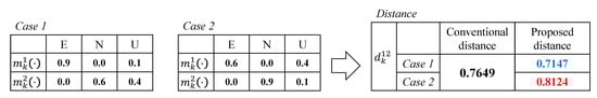
Figure 3.
Example of the proposed distance given , and .
3.1.4. Proposed Data Fusion for Determining Existence
Based on the proposed distance, we leverage technique of the weighted DS combination rule for data fusion [15,23,26,35]. Let us define as the set of vehicles who can communicate with vehicle i and i itself, and as the set of detected objects which are located in vehicle i’s sensing area. Denote the set of vehicles associated with vehicle i who can detect object k by . Suppose the vehicle i currently receives n-th data point. Define the set of vehicles from which vehicle i has received sensing data on object k including i as . We have that . Without loss of generality (WLOG), we assume that j-th data is transmitted from vehicle . Vehicle i calculates distances by (10) between and , and we define similarity matrix [23,25,26], which is given by
where is all-ones matrix. Due to symmetry property from Proposition 1, we have , and thus is a symmetric matrix. Based on (15), we can construct n-th block matrix such that
Let us denote element of as . We define supplementary matrix and credibility matrix [23,26], respectively, where p-th elements are defined by
Note that represents the values from vehicle i, and the derived can be regarded as the weights on -th received confidence for all . Let us define weighted confidence vector about object k at vehicle i as . We calculate based on (17) such that
The elements in (18) are the weighted confidences of E, N, and U. We define the set of elements of as . Next, we can apply the classical DS procedure in (3) to fuse for times [25,26,35,47]. The algorithm for existence calculation is presented in Algorithm 1.
| Algorithm 1 Existence calculation for i about object k |
|
Note that the proposed scheme has polynomial time complexity, which enables its real-time data fusion. The DS rule in general has high computation complexity for data fusion, , which is a main drawback. However, we have 3 elements in , and thus the complexity of calculating the DS rule is . Specifically, the vehicles which detect object k participate in the data fusion, thus vehicle i can obtain the fused output with complexity for each time instant, which in turn we have complexity in the worst case due to . Furthermore, the considered data fusion scheme is valid irrespective of the order of data arrivals as well.
Proposition 2.
Given a set of data points, let and be the arbitrary order of data points where for , and we denote corresponding outputs as and , respectively. Then, we have .
Proof of Proposition 2.
Suppose that vehicle i receives n-th data. We suppose that there are different data arrival orders which are denoted by and , . The hat and check symbols denote the notations related to and , respectively, e.g., and are similarity block matrices in (16) corresponding to and . WLOG, we focus on the data comes from vehicle j. Let us define the order of this data in and as and , respectively. For -th data in , we can express the associated element in supplementary matrix such that
The equalities in (19) and (20) come from the definitions in (15) and (17), respectively. The third equality in (21) holds due to the symmetry of the proposed distance. Finally, we can derive the last equality, as the both -th and -th data refer to the same information from vehicle j. Therefore, we have that
We can apply this process to all the data points, which results in the same weighted output irrespective of any arrival order. □
We can extend Proposition 2 for any order of data points, which results in that given a set of data points, we have the same final output irrespective of the order of fusion. This property guarantees an independence of the data fusion scheme. In other words, as it is a data-driven fusion method, we can focus on the data synthesis rather than external influence such as channel condition, etc. Finally, we determine the existence of object if the calculated result from Algorithm 1 is greater than the predefined threshold , . Next, we proceed to the decision-making for object classification.
3.1.5. Proposed Data Fusion for Object Classification
Next, we consider the object classification process. The frame of discernment for classification is given by the set of objects in the roads, e.g., ={Sedan, SUV, Pedestrian, Bicycle,. Let be the output from object detectors of vehicle i using about class X for object k. We define the set of outputs as . Any object detector providing confidence value for each element in can be applied, e.g., deep neural networks [48], classified vector quantization [49], and k-nearest neighbor [50]. In general, the outputs from the object detection system are not suitable for direct use as confidences [51]. Instead, we apply temperature scaling technique [51] to classifier output, and the calibrated result is defined by
where temperature T is a control parameter. We can tune the deviation among confidences by adjusting the parameter T. This adjustment allows the result to be “soft” while preserving the existing confidence [52]. The classifier assigns confidence (BPA) to each element of , and it satisfies the conditions in (1) and (2). It is reasonable for a classifier to produce distinct probabilities for each candidate class instead of a single output across multiple classes. Therefore, we have the same number of focal elements to .
Next, we will calculate the distance of confidences as in (10) using calibrated confidences. Assume that vehicle i receives n-th data point. Note that only the vehicles who identify “existence” with respect to object k can have the corresponding class confidences, which is defined by . The same procedure in (15)–(18) is applied to obtain the weighted confidences, and the DS combination is performed with respect to the weighted confidences for times. Let us denote the obtained DS combination results for classification as . Finally, we choose the class with the highest confidence in the estimated class given by
where is the class decided at vehicle i about object k. The classification process is presented in Algorithm 2.
| Algorithm 2 Classification fusion for vehicle i about object k |
|
We can show that the data fusion for classification also has polynomial time complexity as follows. Under the classification fusion, as explained previously, we have independent confidences for each class. Consequently, the valid power set of is equal to , which results in complexity to calculate the distance between confidences. Therefore, in total, the complexity of the class fusion process is .
The integrated decision-making is outlined in Algorithm 3. The algorithm uses functions of Existence and Class from Algorithms 1 and 2. Given the collected data, vehicle i first validates the existence of the reported object (step 3). If the existence is confirmed (step 4), the algorithm determines the class of the detected object by fusing the shared confidences (step 5). An example is illustrated in Figure 4. There are 3 vehicles, V1–V3, and an object k which is within the sensing ranges of them, e.g., . Unlike V2 and V3, it is impossible for V1 to detect k, as the object is located in the uncertainty area of V1. Moreover, we assume that V3 fails to detect the object due to, e.g., bad weather or sensor malfunctioning. We set the confidences for each vehicle as in the tables in Figure 4. As only V2 recognizes the object, it has class confidences, i.e., . In this case, through inter-vehicle communications, V1 receives the detection results, then verify the existence of the object. From Algorithm 3, V1 can derive the final outputs for existence and class as and , respectively. We set , thus V1 is able to not only indirectly detect the presence of the object, but also find the class of the object.
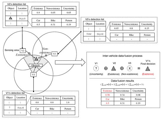
Figure 4.
Example of multisource inter-vehicle data fusion process.
From the experiments in Section 5, we will show that the proposed method operates in real-time, and thus is suitable for the autonomous vehicle environment. Next, we discuss data fusion algorithm for “trajectory” type data.
| Algorithm 3 Decision-making for vehicle i about object k |
|
3.2. Data Fusion for Trajectory Information
The fusion of trajectory information of the object requires a different approach from object type information. The trajectory information for the detected object consists of the measured position, velocity, and the measurement accuracy of the sensor. As explained previously, sensors have an inherent limitation in accuracy. We will use a “multisensor weighted data fusion” technique [53,54,55] so as to combine the reported sensing results and accuracy. The technique provides a fast and robust scheme to overcome the dynamic changes in the vehicular environment.
Let us define and as the velocity of object k measured by vehicle j and the associated accuracy, respectively. These data are transmitted to nearby vehicles through V2V communications. We denote as the fused output based on the data gathered at vehicle i about object k. As in the case of classification, only the vehicles with have the data on object k. Thus, we have that
where is the weight of , and . We assume that the sensor measurements are independent and follow a normal distribution with standard deviation (measurement accuracy) [56,57]. According to the extreme value theory of multivariate function [54,55,58], we can obtain the weights corresponding to the minimum mean square error as below.
The weights in (27) can be interpreted that large variance (low accuracy) results in low weight on measurements. Note that this scheme does not require any prior information, and computing (26) has polynomial time complexity, . In our experiment, on Intel(R) Core(TM) Xeon 2.4 GHz, it takes only s on average in combining 1000 points of velocity data, which is a negligible delay. Likewise, we can combine the location data as well, which are used to estimate the object trajectories.
4. Proposed Collision Warning System and V2V Communications
In this section, we propose a collision warning system and V2V communications integrated with the proposed multisource inter-vehicle data fusion methods.
4.1. Overall System Model
For autonomous vehicles, it is necessary for the embedded collision warning system to quickly perceive the surrounding environment and make decisions. In Figure 5, we illustrate an overall architecture of the proposed collision warning system. We summarize the components of the system as follows. Each vehicle obtains raw data from the equipped sensors such as cameras and radars. Through the object detection process, the object class and its confidences are extracted from the raw data. The trajectory information such as location and velocity are tagged to the object information in real-time. Next, we propose a compact message format for communications to achieve low latency. The encapsulated messages is shared via V2V communication, which provides high data rates and reliability such as DSRC. Next, the aforementioned data fusion algorithms are applied to determine the states of the detected objects. Based on them, the future trajectories of the detected objects are estimated by Kalman filter with cosine effect compensation [59,60]. From the estimated trajectories, the proposed system warns an imminent collision. In this paper, we mainly consider collision warning protocol of the system in detail.
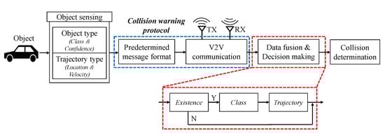
Figure 5.
Proposed collision warning system.
4.2. Object Sensing
Let us consider methods to obtain object type data. Recently, LiDAR-based autonomous vehicle systems have been investigated [31,32,61]. However, due to its high cost [62], most of commercial vehicles such as Tesla and Mercedes-Benz adopt the computer vision as primary object detection rather than LiDAR [45]. Therefore, in this paper, we mainly consider the vision-based object detection system [63,64].
In addition to object type data, trajectory data including location and velocity can be obtained through the radar [42]. However, to obtain precise measurements, the system requires a supplemental calibration process to compensate measurement errors caused by “cosine effect” [59,60,65]. The radar can measure relative speed of the object precisely if the target moves directly in a direction of radar signal. Otherwise, the measured value does not coincide with the actual velocity. Let be the angle between the direction of vehicle i’s radar signal and moving direction of object k. Note that information about object k can be obtained by utilizing historic trajectories. We denote the the measured and compensated velocities about object k for i as and , respectively. Then, we can calculate the compensated value by . In the following, we describe how to transmit these data.
4.3. Message Format
The proposed data format is shown in Figure 6. It is composed of the number of detected objects (N), sensor accuracies (A), confidence (L), and trajectory data. The sensor accuracy is in 4-byte floating point format which contains vision sensor accuracy. The rest are used to set uncertainty of confidences and calculate (26) and (27). Next, the size of confidence part varies depending on the predetermined list of classes, , and we allocate 2 bytes of short data type for each class. The position of the detected object is 24 bytes long consisting of longitude , latitude , and height , which follows the GPS coordination. We use the float data type of 4 bytes for conveying velocity information. The aforementioned field is repeated for N times, thus the size of the entire packet is given by bytes.
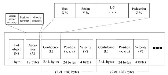
Figure 6.
Proposed message format.
Next, we consider the latency of transmitting vehicle information in the proposed message format. Suppose we use a standard SAE 2735 Basic Safety Message (BSM) format [66] which contains ID, position, speed, heading, etc. We will set the basic BSM to be 500 bytes long, which consists of 300 bytes for the default size of BSM [67,68] plus reserved space for other application such as high-end security. If the system classifies 16 categories and detects 20 objects , the proposed entire safety message is about 1.7 Kbytes, which takes only a few milliseconds in existing V2V communications such as DSRC [11].
4.4. V2V Communication Systems
In this section, we investigate V2V communication system to share the data. Specifically, we define a V2V communication process to maintain the information up to date as possible, and take full advantage of the previously presented data fusion scheme.
Each vehicle is equipped with cameras that record surroundings in F frame-per-second (FPS). We denote k-th video frame as . For a general video, F is fixed, e.g., . In each frame, the vehicle performs object detection, and the result is broadcast periodically every 100 ms according to the standard [69]. Likewise, the detection results of other vehicles arrive periodically. For vehicle i, the data fusion output with respect to k-th frame and set of vehicles from which the data is successfully received, X, is denoted by . We describe the proposed data communication process with an example presented in Figure 7 as follows.
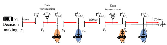
Figure 7.
Example of the considered data communication system and real-time data fusion process. V1 can receive several data within the predetermined cycle (100ms), and a decision-making algorithm updates the fused output in real-time.
- (i)
- Data transmission: at each round, the vehicle transmits the most recently obtained result rather than the combined one, i.e., for the second transmission, V1 sends instead of . This is because of protecting originality and avoiding data contamination.
- (ii)
- Data fusion and update: for every frame, as soon as the vehicle acquires the sensing result, the data combination between the acquired and received data is performed using the data fusion method proposed in Section 3. In this process, note that every received data has an expiration time of 100 ms, i.e., if a new data is not received within 100 ms from the same vehicle, the data is deleted. This case implies that either the transmitted message is obstructed or the vehicle has left the area of interest. In both cases, it can be considered that the data is invalid. For instance, between and , V1 updates its data fusion output as rather than as there is no new data from V2 and the stored data is expired.
In order to implement this procedure in practice, data fusion should be completed within a short time. Nevertheless, the proposed data fusion method is feasible due to low complexity. Furthermore, from Proposition 2, the vehicle no longer has to consider the order of fusion.
4.5. Collision Determination
The fused output of the trajectory information can be applied to estimate the future trajectory of the detected objects. However, in practice, as the measurement has certain level of noise, it is hard to predict trajectories of vehicles correctly. Therefore, we employ a Kalman filter for noise mitigation and precise estimation [70]. We assume that the sensors monitor nearby objects with time interval which is identical to regular video frame. For simplicity, we consider 2-dimensional case mainly in this section, and it can be extended to 3-dimension simply with the same manner. The state and control input of Kalman filter at time t are defined by and , respectively, which consists of x-y coordinates of positions , velocities , and accelerations such that
Let us denote the measurements of position and velocity at time t as . Then, the process dynamics can be expressed as
where and represent process and measurement noises which are white and independent normal distributions with zero mean and noise covariance matrices Q and R, respectively, i.e., and . From (28) and (29), we can estimate trajectory of objects precisely [71].
Next, in order to determine collision, we define the “safety area” of the objects [31,72,73], which is a circle of radius as depicted in Figure 8. Note that under the proposed system, we can determine collisions precisely by utilizing class information. We decide an accident when safety areas of objects and ego-vehicle are overlapped. In other words, along with the estimated trajectories, vehicles examine whether the safety areas overlap, and the anti-collision system would be triggered if an collision is predicted.
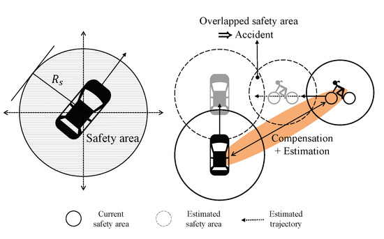
Figure 8.
Safety area and collision determination.
5. Simulation and Experimental Results
In this section, we evaluate the performance of the proposed systems. First, we investigate the latency and improvement of the proposed data fusion schemes. Second, we test for accident scenarios using real-world data. The first scenario concerns predicting accidents caused by blind spots, which can be avoided using V2V communications. The second scenario shows how an erroneous detection can be corrected.
5.1. Simulation Results: Performance Evaluation of Data Fusion Schemes
We first evaluate the delays for the proposed data fusion schemes in Section 3. The simulations are performed on Intel(R) Core(TM) Xeon 2.4 GHz using MATLAB R2014a. We calculate average latency of performing Algorithms 1 and 2, and trajectory data fusion in (26) and (27) to synthesize randomly generated 10 data points for 1000 iterations. Specifically, to satisfy conditions in (1) and (2), the confidence for existence, , is modeled by normal distribution , and the rest are divided into equally for “nonexistence” and “uncertainty”, i.e., . We consider 16 classes, and the corresponding confidences are also generated according to . As a representative, velocity is mainly considered for trajectory type data, which follows [74]. The results are presented in Table 1.

Table 1.
Time consumptions of the proposed data fusion schemes for 10 data points.
Obviously, the data fusion for object type data takes larger calculation time compared to that of trajectory type. Nevertheless, the latency is only about 1 ms for entire data fusion processes, which demonstrates that the proposed data fusion scheme can operate in real-time.
Next, we compute the performance of the proposed scheme in terms of the false negative rate (FNR) defined by
where “true positive” and “false negative” are existence and nonexistence decisions conditional on the existence of object, respectively. We assume that there is an object and 10 vehicles. Each vehicle has one sensor which is in either normal or defective state. Depending on the state of the sensor, vehicles allocate the confidence in existence or nonexistence according to normal distribution with . The rest are divided into other elements uniformly to satisfy the condition in (2), e.g., a vehicle i with normal sensor can have .
In Figure 9, we plot the average FNR values for 10,000 iterations by changing the number of normal sensors. We compare the proposed scheme with classic DS, the weighted DS based on Jousselme distance [25], and the modified DS scheme presented in [26]. As shown in Figure 9, in all cases, the proposed schemes outperform the other data fusion methods in terms of reducing FNR. Specifically, for five normal sensors case, our method can reduce FNR about 18% compared to all the baselines. In addition, the proposed scheme achieves FNR reductions over classic DS (64.8%), Ref. [25] (50.9%), and [26] (65.5%) for seven normal sensors case. This result shows that we can improve the driver’s safety, even if there are high conflicts among confidences. In the following, we experiment how the proposed collision warning scheme can prevent from predicted accidents in real-world.
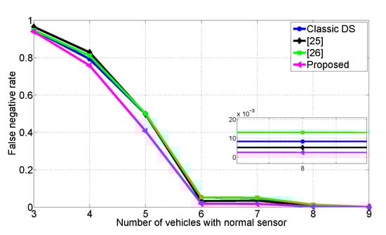
Figure 9.
Comparisons of the false negative rates.
5.2. Experimental Parameters
The two different image sensors (camera) supporting HD (1280 × 720) and full HD (1920 × 1080) resolutions videos with 30 FPS are used to capture real-time vehicular environment. A YOLOv3 [48] is exploited to object detection and classification. We consider 5.9 GHz DSRC network for V2V communication. For compatibility, we consider the proposed packet header contains detection results encapsulated with the basic payload of 500 bytes [75]. The packet is transmitted in 10 Hz period, which is applicable for safety message formats such as Cooperative Awareness Message (CAM), Decentralized Environmental Notification Message (DENM), and BSM used in DSRC. We consider the weighted similarity matrix which has elements such that . The collision occurrence scenarios are modeled by MATLAB on Intel(R) Core(TM) Xeon 2.4 GHz with NVIDIA GeForce 1080Ti GPU. The detailed experimental parameters are presented in Table 2.
Table 2.
Experimental parameters.
5.3. Experimental Result 1: Anti-Collision via V2V
In this scenario, we perform experiments of the proposed anti-collision system with real-world data. As shown in Figure 10a–c, V1 cannot recognize the pedestrian who suddenly appears from an uncertainty area caused by parking cars in a narrow street. However, V2, which comes from the opposite site, is able to detect the pedestrian. The actual images of vehicles’ front view are presented in Figure 10a,b including detection results. A top-view illustration is depicted in Figure 10c. V1 with 36 km/h and V2 with 47 km/h speed drive and a distance between them is about 20 m. A pedestrian walks westwards as 5.5 km/h in 15 m away from V1.
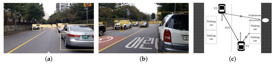
Figure 10.
Collision scenario: (a) Front image of V1 which cannot detect a pedestrian. (b) Front image of V2 which can detect a pedestrian. (c) Top-view illustration of this scenario.
In Figure 11, we plot the measured and estimated values of position, velocity, and calculated acceleration of the pedestrian. In Figure 11b, it is shown that the cosine effect compensation can have a high impact on measurements. As pedestrian and V2 come closer, the angle between them increases, which causes the measured velocities to be smaller than actual values. It can be seen that the estimated values are quite close to ground truth values. The precise estimations in Figure 11a,b result in correct acceleration values (direction) as in Figure 11c.
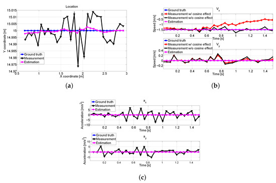
Figure 11.
The received measurement and estimated trajectory about pedestrian at V1: (a) Position comparison. (b) Measured and estimated velocities about x and y axes with and without cosine effect compensation. (c) Comparisons of the calculated acceleration (direction).
Next, we explore how confidences of V1 change over time. We assume that the current frame of V1 and V2 starts at . In this frame, V2 detects seven objects including the pedestrian, which takes 22.46 ms. The detection outcome is encapsulated as the proposed format with 1053 bytes. The delay is only 4.68 ms. As soon as V1 receives data from V2 at ms, the data fusion is performed. As the pedestrian is located in the uncertainty area of V1, we set confidences to . V1 takes 0.88 ms of processing time in the decision-making, prediction, and the decision to issue warning. In addition, the data fusion system returns the highest confidence on the detection of a person. The whole decision process takes only about 27.9 ms. During the process, the confidence on existence changes from 0.0 to 0.66. We impose 0.5 threshold to determine existence of object. The detailed changes in confidences are illustrated in Figure 12; it shows that V1 can start to decelerate after moving by the distance of only 0.27 m even if V1 cannot directly recognize the pedestrian. The detailed results are addressed in Table 3.
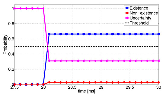
Figure 12.
Changes of confidences about for V1.
Table 3.
Experimental results for the anti-collision case.
Finally, we investigate a collision scenario through the environment modeling as shown in Figure 13. Each object has own safety area, e.g., car has 4.8 m and human is set to 0.5 m. Prediction line indicates future trace until 7 s later, and star dots imply that the accident is expected to happen when moving objects reach those locations. Vehicles are assumed to decelerate with 5 m/ [76]. Figure 13b,c shows the locations of objects without and with the proposed system only after 1.2 s, respectively. In Figure 13b, we can find that an accident occurs between V1 and pedestrian. On the other hand, V1 can slow down its speed by receiving data from V2, and avoids the predicted collision as shown in Figure 13c. From experimental results, we show that the proposed inter-vehicle data fusion takes less than 30 ms from object detection to decision-making. In addition, the existence of the pedestrian in blind spot can be identified by the proposed data fusion scheme. These results demonstrate that we can prevent from the predicted accident in real-time.
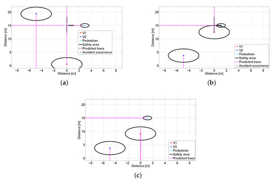
Figure 13.
Snapshots of the scenario modeling: (a) Traces at s. (b) Traces at s without the proposed system. (c) Traces at s with the proposed system.
5.4. Experimental Result 2: Sensing Failover
The next scenario concerns a detection failover through V2V cooperation. As shown in Figure 14, V1 with constant speed of 50 km/h is moving in a narrow space. However, V2 driving in 5 m/ cannot obtain a clear video of V1 due to broken sensor. Therefore, in this case, V1 is regarded as “nonexistence” rather than “uncertainty” by V2, which represents a false negative error [44]. In addition, we assume that V1 cannot communicate with other vehicles due to a malfunction of the communication tools or lack of communication capability. We assume that there are similar problem at V3, i.e., it is hard to obtain clear image on V1. Under this set-up, V2 cannot perceive the movement of V1 at all, and the crash of V1 and V2 is imminent. However, the other cars (V4, V5) located at nearby V1 can recognize the movement of V1 as presented in Figure 14e,f. They transmit this information to the V2 from which the accident can be avoided. The cameras equipped at V2–V5 record V1’s movement simultaneously. We manipulated cameras at V2 and V3 so that they produce blurred videos. Figure 14a,c shows the original clear front views, and Figure 14b,d shows the blurred images at the same time.
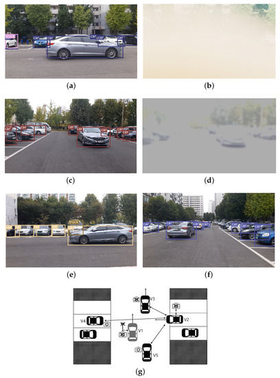
Figure 14.
The video images captured at vehicles and detection results: (a) The original image at V2. (b) The blurred image at V2. (c) The original image at V3. (d) The blurred image at V4. (e) The front view of V4. (f) The front view of V5. (g) Top view illustration.
We compare the measurements and estimation of V1 in Figure 15. Due to the dynamics of V1, the angles between nearby vehicles are changed, which results in inaccurate measurements as shown in Figure 15b. However, Figure 15a–c demonstrates that we obtain precise estimation values by the proposed scheme, and the predicted collisions are avoided.
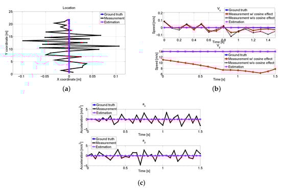
Figure 15.
V2’s combined measurement and estimated trajectory results about V1: (a) Position comparison. (b) Measured and estimated velocities with respect to x and y axes with and without compensation. (c) Calculated acceleration comparisons.
We demonstrate how the confidences change as data sources are added in Figure 16. Especially, we compare the performance of the proposed scheme with the conventional weighted data fusion method exploiting Jousselme’s distance. For abnormal states of V2 and V3, we assume that they have high confidence in “nonexistence” about V1, and the other vehicles are set to have confidence in existence of V1 as 0.7 and 0.9, respectively. In Figure 16a,b, we plot changes of confidences for the proposed and existing weighted DS schemes, respectively. The detailed parameters and experimental results are presented in Table 4. As the data are received sequentially, we can find that the confidence in existence is changed in both figures. However, under the baseline scheme, the final confidence on existence is 0.48, which in turn makes V2 decide “nonexistence”. Contrary to this, the proposed scheme shows 0.58 confidence in existence, thus V2 can recognize V1 successfully. From this result, it is shown that the proposed scheme can reduce the false negative error as compared to the conventional data fusion method.

Figure 16.
Confidence comparison: (a) Changes of the confidences based on the proposed data fusion scheme. (b) Changes of the confidences under the weighted data fusion scheme.
Table 4.
Experimental results for the sensing failover case.
Next, we consider latency. The maximum packet length is 993 bytes, which requires only 4.4 ms to receive the packet, and we have 21 ms processing delay for detection. It takes 0.85 ms on average for V2 to perform decision-making including the estimation of future trajectory of V1. Moreover, V2 decides that the target object is a car. In total, only 29.36 ms is required until V2 begins decelerating, which is much shorter than human reaction time.
An environment modeling for this scenario is shown in Figure 17. As shown in Figure 17b, it is predicted that the accident will happen after 0.7 s. However, under the proposed system, V2 can stop as soon as recognizing movement of the V1 as in Figure 17c.
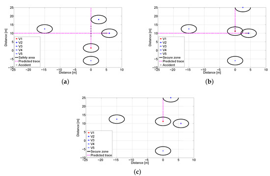
Figure 17.
Environment modeling: (a) Traces at s. (b) Traces at s without the anti-collision system. (c) Traces at s with the proposed system.
6. Conclusions
In this paper, we studied a real-time inter-vehicle data fusion scheme for autonomous vehicle safety which combines multiple sensing results transmitted by adjacent vehicles through V2V communication. First, we proposed a novel metric to measure distance between conflicting confidences on the detected event. We considered a new similarity matrix which takes asymmetric weights of the existence of an object which can be flexibly adjusted depending on its importance. Our approach is applicable to autonomous vehicle by reducing fault diagnosis in vehicular environment, especially false negative errors. According to the proposed distance measure, the weighted DS combination was used to fuse multiple confidences. It was shown that the proposed data fusion scheme has polynomial time complexity, which enables real-time combination of confidences. From simulation, we also show that the proposed scheme can work in real-time and achieve a lower false negative rate compared to both the classical and existing weighted DS fusion schemes. By conducting real-world experiments, we show that the accidents can be prevented by our method. Moreover, even when the ego-vehicle measurements are incorrect, the proposed system can overcome sensing failures through the real-time data fusion via inter-vehicle cooperation.
For future work, we plan to investigate collision avoidance maneuver based on vehicle kinematic model which can be utilized in real-world scenarios such as overtaking and lane changing. As an application of this technique, we will consider a compensation method for trajectory estimation errors by comparing possible maneuvers and estimated movement. Moreover, precise mapping of the surrounding environment is required for reliable maneuver. We also plan to use the data obtained from the vision sensors with the deep learning-based Simultaneous Localization and Mapping (SLAM) method for future research.
Author Contributions
Conceptualization, I.-S.C. and S.J.B.; formal analysis, I.-S.C. and S.J.B.; methodology, I.-S.C. and S.J.B.; investigation, I.-S.C. and S.J.B.; validation, I.-S.C. and S.J.B.; software, I.-S.C. and Y.L.; data curation, I.-S.C. and Y.L.; project administration, S.J.B.; writing—original draft preparation, I.-S.C. and Y.L.; writing—review and editing, S.J.B. All authors have read and agreed to the published version of the manuscript.
Funding
This research was supported by the Korean MSIT (Ministry of Science and ICT), under the National Program for Excellence in SW (2015-0-00936) and under the ICT Creative Consilience program (IITP-2020-0-01819) supervised by the IITP (Institute for Information & communications Technology Planning & Evaluation). This research was also supported by the National Research Foundation of Korea (NRF) grant funded by the Korea government (MSIT) (No. 2018R1A2B6007130).
Conflicts of Interest
The authors declare no conflict of interest.
References
- Singh, S. Critical reasons for crashes investigated in the national motor vehicle crash causation survey. In Traffic Safety Facts-Crash Stats; NHTSA: Washington, DC, USA, 2015. [Google Scholar]
- Fagnant, D.J.; Kockelman, K. Preparing a nation for autonomous vehicles: Opportunities, barriers and policy recommendations. Transp. Res. Part A Policy Pract. 2015, 77, 167–181. [Google Scholar] [CrossRef]
- Betz, J.; Heilmeier, A.; Wischnewski, A.; Stahl, T.; Lienkamp, M. Autonomous Driving-A Crash Explained in Detail. Appl. Sci. 2019, 9, 5126. [Google Scholar] [CrossRef]
- Lee, K.; Kum, D. Collision avoidance/mitigation system: Motion planning of autonomous vehicle via predictive occupancy map. IEEE Access 2019, 7, 52846–52857. [Google Scholar] [CrossRef]
- Aghav, J.; Hirwe, P.; Nene, M. Deep Learning for Real Time Collision Detection and Avoidance. In Proceedings of the International Conference on Communication, Computing and Networking, Chandigarh, India, 23–24 March 2017. [Google Scholar]
- Nobis, F.; Geisslinger, M.; Weber, M.; Betz, J.; Lienkamp, M. A Deep Learning-based Radar and Camera Sensor Fusion Architecture for Object Detection. In Proceedings of the 2019 Sensor Data Fusion: Trends, Solutions, Applications (SDF2019), Bonn, Germany, 15–17 October 2019; pp. 1–7. [Google Scholar]
- Fukatsu, R.; Sakaguchi, K. Millimeter-Wave V2V communications with cooperative perception for automated driving. In Proceedings of the 2019 IEEE 89th Vehicular Technology Conference (VTC2019-Spring), Kuala Lumpur, Malaysia, 28 April–1 May 2019; pp. 1–5. [Google Scholar]
- Perfecto, C.; Del Ser, J.; Bennis, M.; Bilbao, M.N. Beyond WYSIWYG: Sharing contextual sensing data through mmWave V2V communications. In Proceedings of the 2017 European Conference on Networks and Communications (EuCNC), Oulu, Finland, 12–15 June 2017; pp. 1–6. [Google Scholar]
- Jung, C.; Lee, D.; Lee, S.; Shim, D.H. V2X-Communication-Aided Autonomous Driving: System Design and Experimental Validation. Sensors 2020, 20, 2903. [Google Scholar] [CrossRef]
- Yang, X.; Liu, L.; Vaidya, N.H.; Zhao, F. A vehicle-to-vehicle communication protocol for cooperative collision warning. In Proceedings of the First Annual International Conference on Mobile and Ubiquitous Systems: Networking and Services, Boston, MA, USA, 26 August 2004; pp. 114–123. [Google Scholar]
- MacHardy, Z.; Khan, A.; Obana, K.; Iwashina, S. V2X access technologies: Regulation, research, and remaining challenges. IEEE Commun. Surv. Tutor. 2018, 20, 1858–1877. [Google Scholar] [CrossRef]
- IEEE 1609 Working Group. IEEE Standard for Wireless Access in Vehicular Environments (WAVE)-Multi-Channel Operation; IEEE Std 1609.4-2016; IEEE Standards Associations: New York, NY, USA, 2016. [Google Scholar]
- Azzaoui, N.; Korichi, A.; Brik, B.; Fekair, M.E.A.; Kerrache, C.A. Wireless communication in internet of vehicles networks: DSRC-based Vs cellular-based. In Proceedings of the 4th International Conference on Smart City Applications, Casablanca, Morocco, 2–4 October 2019; pp. 1–6. [Google Scholar]
- Mahmood, A.; Zhang, W.E.; Sheng, Q.Z. Software-defined heterogeneous vehicular networking: The architectural design and open challenges. Future Internet 2019, 11, 70. [Google Scholar] [CrossRef]
- Chen, J.; Ye, F.; Jiang, T. Numerical analyses of modified DS combination methods based on different distance functions. In Proceedings of the 2017 Progress in Electromagnetics Research Symposium-Fall (PIERS-FALL), Singapore, 19–22 November 2017; pp. 2169–2175. [Google Scholar]
- Fragkiadakis, A.G.; Siris, V.A.; Petroulakis, N.E.; Traganitis, A.P. Anomaly-based intrusion detection of jamming attacks, local versus collaborative detection. Wirel. Commun. Mob. Comput. 2015, 15, 276–294. [Google Scholar] [CrossRef]
- Shafer, G. A Mathematical Theory of Evidence; Princeton University Press: Princeton, NJ, USA, 1976; Volume 42. [Google Scholar]
- Ma, W.; Jiang, Y.; Luo, X. A flexible rule for evidential combination in Dempster-Shafer theory of evidence. Appl. Soft Comput. 2019, 85, 105512. [Google Scholar] [CrossRef]
- Chen, Q.; Aickelin, U. Anomaly detection using the Dempster-Shafer method. In Proceedings of the International Conference on Data Mining 2006, Las Vegas, NV, USA, 26–29 June 2006; pp. 232–240. [Google Scholar]
- Siaterlis, C.; Maglaris, B. Towards multisensor data fusion for DoS detection. In Proceedings of the 2004 ACM Symposium on Applied Computing, Nicosia, Cyprus, 14–17 March 2004; pp. 439–446. [Google Scholar]
- Sakr, A.H.; Bansal, G. Cooperative localization via DSRC and multisensor multi-target track association. In Proceedings of the 2016 IEEE 19th International Conference on Intelligent Transportation Systems (ITSC), Rio de Janeiro, Brazil, 1–4 November 2016; pp. 66–71. [Google Scholar]
- Li, T.; Choi, M.; Guo, Y.; Lin, L. Opinion mining at scale: A case study of the first self-driving car fatality. In Proceedings of the 2018 IEEE International Conference on Big Data (Big Data), Seattle, WA, USA, 10–13 December 2018; pp. 5378–5380. [Google Scholar]
- Khan, N.; Anwar, S. Improved Dempster-Shafer Sensor Fusion using Distance Function and Evidence Weighted Penalty: Application in Object Detection. In Proceedings of the ICINCO 2019, Prague, Czech Republic, 29–31 July 2019; pp. 664–971. [Google Scholar]
- Jousselme, A.L.; Grenier, D.; Bosse, E. A new distance between two bodies of evidence. Inf. Fusion 2001, 2, 91–101. [Google Scholar] [CrossRef]
- Yong, D.; Shi, W.; Zhu, Z.; Qi, L. Combining belief functions based on distance of evidence. Decis. Support Syst. 2004, 38, 489–493. [Google Scholar] [CrossRef]
- Chen, L.; Diao, L.; Sang, J. Weighted evidence combination rule based on evidence distance and uncertainty measure: An application in fault diagnosis. Math. Probl. Eng. 2018, 2018, 5858272. [Google Scholar] [CrossRef]
- Cheng, C.; Xiao, F. A New Distance Measure of Belief Function in Evidence Theory. IEEE Access 2019, 7, 68607–68617. [Google Scholar] [CrossRef]
- Aeberhard, M.; Paul, S.; Kaempchen, N.; Bertram, T. Object existence probability fusion using dempster-shafer theory in a high-level sensor data fusion architecture. In Proceedings of the 2011 IEEE Intelligent Vehicles Symposium (IV), Baden-Baden, Germany, 5–9 June 2011; pp. 770–775. [Google Scholar]
- Claussmann, L.; O’Brien, M.; Glaser, S.; Najjaran, H.; Gruyer, D. Multi-criteria decision making for autonomous vehicles using fuzzy dempster-shafer reasoning. In Proceedings of the 2018 IEEE Intelligent Vehicles Symposium (IV), Suzhou, China, 26–30 June 2018; pp. 2195–2202. [Google Scholar]
- Mouhagir, H.; Cherfaoui, V.; Talj, R.; Aioun, F.; Guillemard, F. Trajectory planning for autonomous vehicle in uncertain environment using evidential grid. In Proceedings of the 20th International Federation of Automatic Control World Congress, Toulouse, France, 9–14 July 2017; pp. 12545–12550. [Google Scholar]
- Laghmara, H.; Boudali, M.-T.; Laurain, T.; Ledy, J.; Orjuela, R.; Lauffenburger, J.-P.; Basset, M. Obstacle Avoidance, Path Planning and Control for Autonomous Vehicles. In Proceedings of the 2019 IEEE Intelligent Vehicles Symposium (IV), Paris, France, 9–12 June 2019; pp. 529–534. [Google Scholar]
- Xu, F.; Liang, H.; Wang, Z.; Lin, L.; Chu, Z. A Real-Time Vehicle Detection Algorithm Based on Sparse Point Clouds and Dempster-Shafer Fusion Theory. In Proceedings of the 2018 IEEE International Conference on Information and Automation (ICIA), Fujian, China, 11–14 August 2018; pp. 597–602. [Google Scholar]
- Liu, W. Analyzing the degree of conflict among belief functions. Artif. Intell. 2006, 170, 909–924. [Google Scholar] [CrossRef]
- Zhu, J.; Wang, X.; Song, Y. A new distance between BPAs based on the power-set-distribution pignistic probability function. Appl. Intell. 2018, 48, 1506–1518. [Google Scholar] [CrossRef]
- Wang, J.; Hu, Y.; Xiao, F.; Deng, X.; Deng, Y. A novel method to use fuzzy soft sets in decision making based on ambiguity measure and Dempster-Shafer theory of evidence An application in medical diagnosis. Artif. Intell. Med. 2016, 69, 1–11. [Google Scholar] [CrossRef]
- Jousselme, A.L.; Liu, C.; Grenier, D.; Bosse, E. Measuring ambiguity in the evidence theory. IEEE Trans. Syst. Man Cybern. Part A Syst. Hum. 2006, 36, 890–903. [Google Scholar] [CrossRef]
- Hafner, M.; Cunningham, D.; Caminiti, L.; Del Vecchio, D. Automated vehicle-to-vehicle collision avoidance at intersections. In Proceedings of the World Congress on Intelligent Transport Systems, Orlando, FL, USA, 16–20 October 2011. [Google Scholar]
- Deng, R.; Di, B.; Song, L. Cooperative Collision Avoidance for Overtaking Maneuvers in Cellular V2X-Based Autonomous Driving. IEEE Trans. Veh. Technol. 2019, 68, 4434–4446. [Google Scholar] [CrossRef]
- Chen, M.; Zhan, X.; Tu, J.; Liu, M. Vehicle-localization-based and DSRC-based autonomous vehicle rear-end collision avoidance concerning measurement uncertainties. IEEJ Trans. Electr. Electron. Eng. 2019, 14, 1348–1358. [Google Scholar] [CrossRef]
- Aparicio-Navarro, F.J.; Kyriakopoulos, K.G.; Parish, D.J. An on-line wireless attack detection system using multi-layer data fusion. In Proceedings of the 2011 IEEE International Workshop on Measurements and Networking Proceedings (M&N), Anacapri, Italy, 10–11 October 2011; pp. 1–5. [Google Scholar]
- Yu, D.; Frincke, D. Alert confidence fusion in intrusion detection systems with extended Dempster-Shafer theory. In Proceedings of the 43rd Annual Southeast Regional Conference, Kennesaw, GA, USA, 18–20 March 2005; Volume 2, pp. 142–147. [Google Scholar]
- Folster, F.; Rohling, H.; Lubbert, U. An automotive radar network based on 77 GHz FMCW sensors. In Proceedings of the IEEE International Radar Conference, Arlington, VA, USA, 9–12 May 2005; pp. 871–876. [Google Scholar]
- Sentz, K.; Ferson, S. Combination of evidence in Dempster-Shafer Theory; Sandia National Laboratories: Albuquerque, NM, USA, 2002; Volume 4015.
- Saxena, S.; Isukapati, I.K.; Smith, S.F.; Dolan, J.M. Multiagent Sensor Fusion for Connected & Autonomous Vehicles to Enhance Navigation Safety. In Proceedings of the 2019 IEEE Intelligent Transportation Systems Conference (ITSC), Auckland, New Zealand, 27–30 October 2019; pp. 2490–2495. [Google Scholar]
- Van Brummelen, J.; O’Brien, M.; Gruyer, D.; Najjaran, H. Autonomous vehicle perception: The technology of today and tomorrow. Transp. Res. Part C Emerg. Technol. 2018, 89, 384–406. [Google Scholar] [CrossRef]
- Gentle, J.E. Matrix Algebra: Theory, Computations, and Applications in Statistics; Springer: New York, NY, USA, 2007. [Google Scholar]
- Murphy, C.K. Combining belief functions when evidence conflicts. Decis. Support Syst. 2000, 29, 1–9. [Google Scholar] [CrossRef]
- Redmon, J.; Farhadi, A. Yolov3: An incremental improvement. arXiv 2018, arXiv:1804.02767. [Google Scholar]
- Zhang, B.; Zhou, Y.; Pan, H. Vehicle classification with confidence by classified vector quantization. IEEE Intell. Transp. Syst. Mag. 2013, 5, 8–20. [Google Scholar] [CrossRef]
- Amato, G.; Falchi, F.; Gennaro, C. Geometric consistency checks for kNN based image classification relying on local features. In Proceedings of the Fourth International Conference of Similarity Search and Application, Lipari, Italy, 30 June–1 July 2011; pp. 81–88. [Google Scholar]
- Guo, C.; Pleiss, G.; Sun, Y.; Weinberger, K.Q. On calibration of modern neural networks. In Proceedings of the 34th International Conference on Machine Learning, Sydney, Australia, 6–11 August 2017; pp. 1321–1330. [Google Scholar]
- Kull, M.; Nieto, M.P.; Kangsepp, M.; Silva Filho, T.; Song, H.; Flach, P. Beyond temperature scaling: Obtaining well-calibrated multi-class probabilities with Dirichlet calibration. In Proceedings of the 33rd Conference on Neural Information Processing Systems (NeurIPS 2019), Vancouver, BC, Canada, 8–14 December 2019; pp. 12295–12305. [Google Scholar]
- Alotibi, F.; Abdelhakim, M. Anomaly Detection in Cooperative Adaptive Cruise Control Using Physics Laws and Data Fusion. In Proceedings of the 2019 IEEE 90th Vehicular Technology Conference (VTC2019-Fall), Honolulu, HI, USA, 22–25 September 2019; pp. 1–7. [Google Scholar]
- Yan, Z.-Z.; Yan, X.-P.; Xie, L.; Wang, Z. The research of weighted-average fusion method in inland traffic flow detection. In Proceedings of the International Conference on Information Computing and Applications, Qinhuangdao, China, 28–31 October 2011; pp. 89–96. [Google Scholar]
- Wang, Y.; Chen, H.; Zhang, Q.; Lv, H. The application of multiple wireless sensor data fusion algorithm in temperature monitoring system. In Proceedings of the WCSE, Bangkok, Tahiland, 28–30 June 2018; pp. 227–231. [Google Scholar]
- Li, D.; Shen, C.; Dai, X.; Zhu, X.; Luo, J.; Li, X.; Chen, H.; Liang, Z. Research on data fusion of adaptive weighted multisource sensor. CMC Comput. Mater. Contin. 2019, 61, 1217–1231. [Google Scholar]
- Shin, S.-J. Radar measurement accuracy associated with target RCS fluctuation. Electron. Lett. 2017, 53, 750–752. [Google Scholar] [CrossRef]
- Zhang, Z.; Nan, X.; Wang, C. Real-Time Weighted Data Fusion Algorithm for Temperature Detection Based on Small-Range Sensor Network. Sensors 2019, 19, 64. [Google Scholar] [CrossRef] [PubMed]
- Mandava, M.; Gammenthaler, R.S.; Hocker, S.F. Vehicle Speed Enforcement Using Absolute Speed Handheld Lidar. In Proceedings of the 2018 IEEE 88th Vehicular Technology Conference (VTC-Fall), Chicago, IL, USA, 27–30 August 2018; pp. 1–52. [Google Scholar]
- Weil, C.M.; Camell, D.; Novotny, D.R.; Johnk, R.T. Across-the-road photo traffic radars: New calibration techniques. In Proceedings of the 15th International Conference on Microwaves, Radar and Wireless Communications, Warsaw, Poland, 17–19 May 2004; pp. 889–892. [Google Scholar]
- Shahian Jahromi, B.; Tulabandhula, T.; Cetin, S. Real-Time Hybrid Multi-Sensor Fusion Framework for Perception in Autonomous Vehicles. Sensors 2019, 19, 4357. [Google Scholar] [CrossRef]
- Liu, S.; Tang, J.; Zhang, Z.; Gaudiot, J.L. Computer architectures for autonomous driving. Computer 2017, 50, 18–25. [Google Scholar] [CrossRef]
- Bechtel, M.G.; McEllhiney, E.; Kim, M.; Yun, H. Deeppicar: A low-cost deep neural network-based autonomous car. In Proceedings of the 2018 IEEE 24th International Conference on Embedded and Real-Time Computing Systems and Applications (RTCSA), Hakodate, Japan, 28–31 August 2018; pp. 11–21. [Google Scholar]
- Islam, M.; Chowdhury, M.; Li, H.; Hu, H. Vision-based navigation of autonomous vehicles in roadway environments with unexpected hazards. Transp. Res. Rec. 2019, 2673, 494–507. [Google Scholar] [CrossRef]
- Castro, M.; Iglesias, L.; Sanchez, J.A. Vehicle speed measurement: Cosine error correction. Measurement 2012, 45, 2128–2134. [Google Scholar] [CrossRef]
- SAE. Dedicated Short Range Communications (DSRC) Message Set Dictionary; SAE International: Warrendale, PA, USA, 2009. Available online: https://one.nhtsa.gov/DOT/NHTSA/NRD/Multimedia/PDFs/Crash%20Avoidance/2008/811073.pdf (accessed on 28 September 2020).
- Ahmed-Zaid, F.; Carter, A. Vehicle Safety Communications-Applications VSC-A; First Annual Report December 7, 2006 through December 31, 2007; NHTSA: Washington, DC, USA, 2009.
- Javed, M.A.; Khan, J.Y. Performance analysis of a time headway based rate control algorithm for VANET safety applications. In Proceedings of the 7th International Conference on Signal Processing and Communication Systems (ICSPCS), Gold Coast, Australia, 16–18 December 2013; pp. 1–6. [Google Scholar]
- Huang, X.; Zhao, D.; Peng, H. Empirical study of DSRC performance based on safety pilot model deployment data. IEEE Trans. Intell. Transp. Syst. 2017, 18, 2619–2628. [Google Scholar] [CrossRef]
- Graf, M.; Speidel, O.; Dietmayer, K. Trajectory Planning for Automated Vehicles in Overtaking Scenarios. In Proceedings of the 2019 IEEE Intelligent Vehicles Symposium (IV), Paris, France, 9–12 June 2019; pp. 1653–1659. [Google Scholar]
- Kim, Y.; Bang, H. Introduction to Kalman Filter and Its Applications. In Kalman Filter; IntechOpen: London, UK, 2018; pp. 1–6. [Google Scholar]
- Lee, J.; Kim, G.; Kim, B. Study on the Improvement of a Collision Avoidance System for Curves. Appl. Sci. 2019, 9, 5380. [Google Scholar] [CrossRef]
- Yang, A.; Naeem, W.; Fei, M.; Tu, X. A cooperative formation-based collision avoidance approach for a group of autonomous vehicles. Int. J. Adapt. Control Signal Process. 2017, 31, 489–506. [Google Scholar] [CrossRef]
- Hasch, J.; Topak, E.; Schnabel, R.; Zwick, T.; Weigel, R.; Waldschmidt, C. Millimeter-wave technology for automotive radar sensors in the 77 GHz frequency band. IEEE Trans. Microw. Theory Tech. 2012, 60, 845–860. [Google Scholar] [CrossRef]
- Liu, X.; Jaekel, A. Congestion control in V2V safety communication: Problem, analysis, approaches. Electronics 2019, 8, 540. [Google Scholar] [CrossRef]
- Bokare, P.; Maurya, A. Acceleration-deceleration behaviour of various vehicle types. Transp. Res. Procedia 2017, 25, 4733–4749. [Google Scholar] [CrossRef]


© 2020 by the authors. Licensee MDPI, Basel, Switzerland. This article is an open access article distributed under the terms and conditions of the Creative Commons Attribution (CC BY) license (http://creativecommons.org/licenses/by/4.0/).