An Efficient Radio Frequency Interference (RFI) Recognition and Characterization Using End-to-End Transfer Learning

Abstract

Radio Frequency Interference (RFI) detection and characterization play a critical role in ensuring the security of all wireless communication networks. Advances in Machine Learning (ML) have led to the deployment of many robust techniques dealing with various types of RFI. To sidestep an unavoidable complicated feature extraction step in ML, we propose an efficient Deep Learning (DL)-based methodology using transfer learning to determine both the type of received signals and their modulation type. To this end, the scalogram of the received signals is used as the input of the pretrained convolutional neural networks (CNN), followed by a fully-connected classifier. This study considers a digital video stream as the signal of interest (SoI), transmitted in a real-time satellite-to-ground communication using DVB-S2 standards. To create the RFI dataset, the SoI is combined with three well-known jammers namely, continuous-wave interference (CWI), multi- continuous-wave interference (MCWI), and chirp interference (CI). This study investigated four well-known pretrained CNN architectures, namely, AlexNet, VGG-16, GoogleNet, and ResNet-18, for the feature extraction to recognize the visual RFI patterns directly from pixel images with minimal preprocessing. Moreover, the robustness of the proposed classifiers is evaluated by the data generated at different signal to noise ratios (SNR).

1. Introduction

Recent advances in Software-Defined Radios (SDR) and cognitive networking technologies, as well as increasing the accessible low-cost hardware, have led to most applications becoming dependent on the wireless networks [1]. It provides adversaries with an opportunity to deploy the jamming attacks (also known as the intentional Radio Frequency Interference—RFI) and harm systems that rely on wireless networks [1]. Jamming attacks cause Denial-of-Service (DoS) problems such as slowing browsing websites and downloading files, intensively limiting the number of active voice users, and as a result, network latency [2]. Although the jammers can be launched using simple and cheap technologies, they are hard to defeat due to the large variety of available jammers completely [3].

To guarantee the Quality of Service (QoS) and security of the wireless communication system, a robust RFI detection strategy is required to produce an effective mitigation process [3]. Besides, it is essential to precisely determine the modulation type of SoI combined by any type of RFI. Since Automatic Modulation Classification (AMC) is a significant procedure in communication networks to facilitate the demodulation process at the receiver side [4].

To address this concern, Machine Learning (ML) based techniques have shown promising results in the area of multiclass RFI recognition [5,6] and Automatic modulation classification (AMC) [6]. However, the complex nature of preprocessing tasks such as feature extraction and feature selection in classical ML techniques highly degrades the classification performance regarding efficiency [7]. To tackle this issue, deep learning (DL)-based approaches, as a subfield of ML, have presented outstanding RFI detection results. DL-based techniques include numerous information processing layers in a hierarchical design for either pattern classification or feature extraction [8]. One of the most successful types of DL is Convolutional Neural Networks (CNN), which has been typically used for object detection in computer vision fields, without any prior knowledge regarding the object’s location [9].

The main challenge of DL in supervised learning applications could be the lack of enough data to train the model from scratch. To address this issue, the image-based transfer learning method has gained attraction in the case of an insufficient dataset to create models [10,11]. Transfer learning refers to reuse the pretrained CNN architectures on a prebuild large dataset, such as the ImageNet project [10]. Hence, transfer learning leads to minimizing the training time by considering the pretrained layers of a model [10].

The main contribution of this work is not only specifying the type of received signals but also determining different schemes of digital modulation in the presence of jamming signals in a real-time digital video broadcasting based on DVB-S2 standard using transfer learning. To this end, we propose a hierarchical classification design for RFI classification and AMC by leveraging the benefits of transfer learning technology using pretrained CNNs such as AlexNet, VGG16, GoogleNet, and ResNet18 for feature learning, followed by a fully-connected classifier. This study provides a comparative analysis of these pretrained CNNs with respect to accuracy in the context of transfer learning and consumed training time. We have generated visual representations of the received signals in the time-frequency domain as the input data, which is the magnitude squared of the wavelet transform known as scalogram [12].

In this work, SoI is a video stream transmitted in a digital video broadcasting scenario based on DVB-S2 standard in a real-time Satellite communication (Satcom). We have assumed that SoI is combined with three well-known types of jammers, namely, continuous-wave interference (CWI), multi-CWI (MCWI), and chirp interference (CI), to increase the scenarios complexity and to simulate the realistic situations [5]. As a result, the proposed methodology can precisely determine the type of the received signal, either SoI or a combination of SoI with any other jammers, and also the modulation type of SoI. We have investigated four different types of modulation due to their more applicable in DVB-S2 standard, namely, quadrature phase-shift keying (QPSK), 8-array asymmetric phase-shift keying (8-APSK), 16-array APSK (16-APSK), and 32-array APSK (32-APSK).

The rest of this paper presents the related works in Section 2, the proposed methodology in Section 3, and the simulation results are provided in Section 4. Finally, the paper is concluded in Section 5.

2. Related Works

With the rapid advances of AI technology, DL is also increasingly being applied to the field of RFI and modulation classification. To name a few, in [13], a robust Dl-based technique is proposed known as faster region-based convolutional neural networks (Faster R-CNN) for interference and clutter detection in a high-frequency surface wave radar (HFSWR). To this end, the Range-Doppler (RD) spectrum image is used as the input of the designed network. As a result, the proposed method has a high classification accuracy and a decent detection performance [13].

Z. Yang and et al. have proposed a CNN-based strategy named RFI-Net to detect interference in a five-hundred-meter Aperture Spherical radio Telescope (FAST) [14], that can outperform other techniques such as the U-Net model based on a CNN architecture, k-nearest neighbors (KNN), as well as Sum-Threshold. In [15], two DL-based strategies are used for jamming attack detection, namely deep convolutional neural networks (DCNN) and deep recurrent neural networks (DRNN). In this research, two different jamming attacks, namely, classical wide-band barrage jamming and reference signal jamming, have been analyzed [15]. The results show that the classification accuracy reaches up to 86.1% under a realistic test environment [15].

In [16], three methods, including a Convolutional Long Short-term Deep Neural Network (CLDNN), a Long Short-Term Memory neural network (LSTM), and a deep Residual Network (ResNet) have been proposed to recognize ten different modulation types. The results indicate that the classification accuracy is increased by up to 90% at high SNRs.

Further Principal Component Analysis (PCA) has been deployed to optimize the classification process by minimizing the size of the training dataset [16]. A combination of the transfer learning and a pretrained Inception-ResNetV2 has been presented in [17] to recognize three modulation types, namely Binary Phase Shift Keying (BPSK), QPSK, and 8PSK at SNR equal to 4 dB. As the results illustrate, the classification accuracies to recognize BPSK, QPSK, and 8PSK are 100%, 99.66%, and 96.33% respectively [17].

In [18], a robust hierarchical DNN architecture is presented that performs a hierarchical classification to estimate data type (analog or digital modulation), modulation class, and modulation order. To this purpose, spectrogram snapshots computed from baseband signal in-phase and Quadratic (I/Q) components of the signal are used as the input of the CNN and reach out the performance of 90% at high SNR for most modulation schemes [18]. Yang et al. present an efficient methodology using CNN and Recurrent Neural Networks (RNN) to classify six modulation types under two-channel distortions such as Additive White Gaussian noise (AWGN) and Rayleigh fading [19]. According to the experimental results, the classification precision of the CNN is always close to 100% in AWGN channel [19].

Even in the Rayleigh channel, the minimum classification accuracy still approaches 84%, whereas the maximum value is near 96%. Ref. [20] proposes a robust CNN-based approach that can precisely classify four types of modulation, including BPSK, QPSK, 8PSK, and 16QAM in an orthogonal frequency division multiplexing (OFDM) system under the presence of Phase offset (PO). In [21], CNN and LSTM have been used to solve the AMC problem.

Furthermore, the proposed classifiers that are based on the fusion model in serial and parallel modes are highly beneficial to improving classification accuracy when the SNR is ranging from 0 dB to 20 dB [21]. As is shown, the serial fusion mode has the best performance compared with other modes.

3. Proposed Methodology

This study proposes a DL-based approach for RFI recognition and AMC by benefiting from the transfer learning strategy. The general framework is based on the hierarchical classification in which the first and second levels determine the type of the received signal that is either SoI or a combination of SoI with any of the jamming signals and the modulation type of SoI, respectively [6]. To this end, in the first classification level, a classifier is trained to determine the type of received signals. Further, a classifier is trained per each type of received signal to recognize the modulation type of the combined SoI. Figure 1 demonstrates the proposed methodology, which follows four steps: (1) data acquisition, (2) scalogram computation, (3) Feature extraction using pretrained CNN, and (4) classification. Each step will be fully elaborated in the rest of this section.

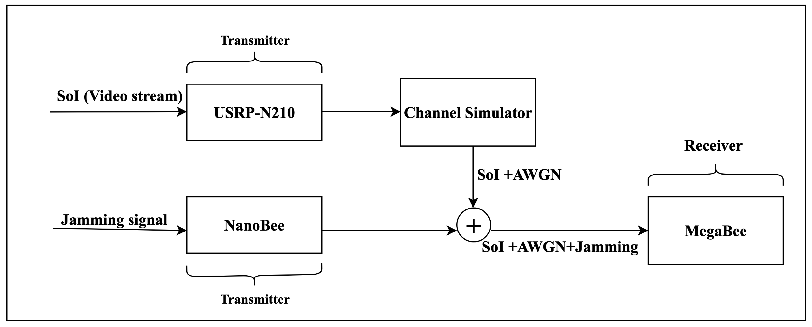
3.1. Data Acquisition Set-Up

As fully explained in [5,6], the desired signal is a video stream, which is modulated and processed by GNU radio and transmitted using a Universal Software Radio Peripheral (USRP-N210) [22]. For modeling a real-time Satcom, the channel simulator (RTLogic T400) [23] is used. Further, the generated jamming signals are combined to SoI by a combiner. Finally, the combined signal is received by a MegaBee modem [5]. Notably, AWGN power can be manually adjusted in the range of −168 to −125 dBm, which is approximately equal to SNR 5 to 12 dB. Figure 2 shows the Real-time RFI data acquisition set-up.

Table 1. Real-time dataset specification.

Characteristic	Value
Total number of observations	4800
Length of each generated signal	32,448 (8 ms)
Sampling frequency	40 × 10${}^6$ Hz
Modulation types	QPSK, 8APSK, 16APSK, and 32APSK
AWGN power	140 dBm ($SNR\cong$ 9 dB)
No. of each class of signals per modulation type	300

presents a summary of the dataset specification generated in [5].

This study analyzes the efficiency of the proposed classification technique in the presence of three jamming signals, such as continuous-wave interference (CWI), multi-CWI (MCWI), and chirp interference (CI) [5].

(1)

Continuous Wave Interference (CWI):

$$CW=exp\left(j2\pi f_{cw}t\right)$$

(1)

where $f_{cw}$ and t represent the center frequency and the duration of interference respectively.

(2)

Multi Continuous Wave Interference (MCWI): In this study, we have considered two-tone CW, which is defined as:

$$MCW=exp\left(j2\pi f_{c_1}t\right)+exp\left(j2\pi f_{c_2}t\right)$$

(2)

where $f_{c_1}$ and $f_{c_2}$ are the center frequencies of each wave.

(3)

Chirp Interference (CI): The CI has been generated according to [24] as follows:

$$Chirp=exp(2\pi \frac{k}{2}{t}^2+2\pi f_{0}t)$$

(3)

where $k=\frac{f_1-f_0}{T}$ so that the signal sweeps from $f_0$ to $f_1$ and T is the sweeping duration.

Note: the center frequencies have been considered to be changed randomly.

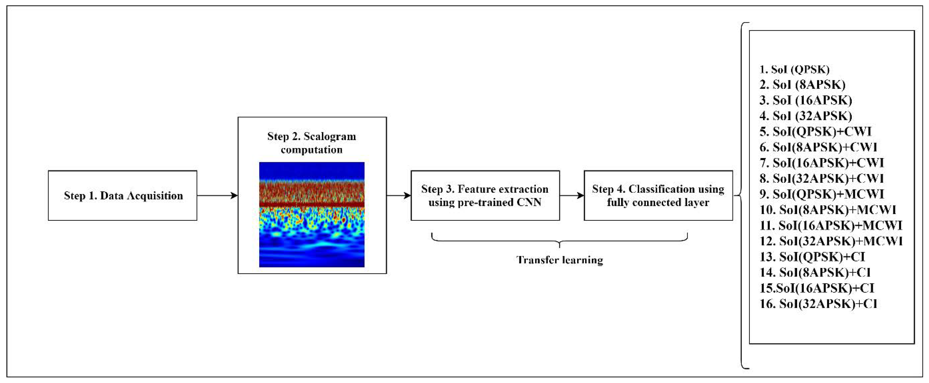
Dataset Generation

This study has considered a visual representation of the received signals in the time-frequency domain using a scalogram as the input data. The scalogram is the squared magnitude of Continuous Wavelet Transform (CWT) and mathematically is defined as [25]:

$$z_x(\alpha ,\tau )=|\frac{1}{\sqrt{\alpha }}{\int }_{-\infty }^{+\infty }x\left(t\right){\mathrm{\Phi }}^{*}(\frac{t-\tau }{\alpha })dt{\left)\right|}^2$$

(4)

where z and ${\mathrm{\Phi }}^{*}$ denote scalogram and the complex conjugate of the mother wavelet function, $\alpha$, and $\tau$ are the oscillatory frequency and shifting position of the wavelet, respectively [25]. CWT is widely applied for nonstationary and transient signal analysis, mainly through its scalogram [26]. The main difference between wavelet transform and short-time Fourier transform (STFT) is that STFT has a fixed signal analysis window whereas the wavelet transform utilizes short windows at high frequencies and long windows at low frequencies [12].

Therefore, the wavelet transform provides superior time and frequency resolution at high and low frequencies [12]. Hence, the wavelet-based analysis is considered an appropriate choice when the signal at hand has high-frequency components for a short duration and low-frequency components for a longer period, as is considered in this study [12]. As shown in Figure 3, the scalogram of SoI and its combination with CWI, CI, and MCWI jammers is computed using the Morse wavelet [27] to calculate the wavelet transform as well as the coherence analysis of the time series. For further processing, the computed scalogram is converted to an RGB image.

3.2. Transfer Learning Process

One of the main applications of transfer learning is feature extraction [28]. In the feature extraction approach, the output from one or more than one layer in the pretrained CNN is used as the input feature vector for the classification phase [29]. Since the deeper layers extract the higher-level features, the layer right before the classification phase can be an appropriate choice for feature extraction [30].

A typical CNN structure consists of two parts; (1) convolutional layers, composed by a stack of the convolutional and the pooling layers to extract the features from the image-based input. (2) a classification part including a set of fully-connected (FC) layers followed by an activation function, like Soft-Max, to classify the images using the extracted features [11]. In the transfer learning process, the classification part can be replaced by a new classifier that fits the application in hand and the model can be tuned using one of the following strategies [11]:

• Training the entire dataset: The pretrained CNN can be trained from scratch using a new dataset. Therefore, a large dataset and lots of computational power are required.
• Training some layers and leaving the others frozen: As the lower layers extract the general features while higher layers represent the most specific features, it can be decided how many layers need to be retrained depending on the application. For a small dataset with a large number of parameters, it is efficient to leave more layers frozen. Because the frozen layers are kept unchanged during the training process to avoid overfitting. On the other hand, for a large dataset with a small number of parameters, training more layers would be reasonable to the new task, since overfitting is not an issue.
• Freezing the convolutional part: In this scenario, the convolutional part can be kept unchanged, and its output can be fed to a new classifier. In other words, the pretrained model is considered as a fixed feature extraction basis, which is beneficial in case of having a small dataset and suffering from a lack of computational power. Notably, in this study, we have applied this strategy.

Notably, the first two strategies highly depend on the learning rate, which defines how much the weights of a network can be adjusted. A small value learning rate can be chosen over a high-value to reduce the risk of losing previous knowledge [11].

3.2.1. Pretrained CNNs

As presented in the previous section, transfer learning refers to the reuse of pretrained CNN architectures on a large dataset. In this study, we have analyzed the efficiency of four well-known CNN architectures, namely, AlexNet [9], GoogleNet [31], ResNet18 [32], and VGG16 [33] regarding classification precision and training time, as you can see below:

• AlexNet: In 2012, AlexNet could outperform other prior architectures in ImageNet LSVRC-2012 competition, designed by the SuperVision group [9]. AlexNet includes five convolutional layers and three FC layers in which Relu is applied after every convolutional and FC layer. In addition, the dropout technique is applied before the first and the second FC layer [9].
• GoogleNet: GoogleNet won ILSVRC 2014 competition with a high precision close to human perception. Its architecture has taken benefits of several small convolutions to reduce the number of parameters drastically. It consists of a 22-layer deep CNN, but it decreased the number of parameters from 60 million (in AlexNet) to 4 million [31].
• VGG: Visual Geometry Group (VGG) is a CNN proposed by the University of Oxford [33] to improve AlexNet by replacing large kernel-sized filters with multiple 3 by 3 kernel-sized filters one after another. VGG16 was trained for weeks and was using NVIDIA Titan Black GPU [33].
• ResNet: Residual Neural Network (ResNet) presented an outstanding performance in ILSRVC 2015 [32]. The Residual network directly copies the input matrix to the second transformation output and sums up the output in final ReLU function [32].

It should be taken into account that the output of the last layer of the convolutional structure before the classification layer has been used as the feature set for the designed classification; “fc8” for AlexNet and VGG16, “loss3-classifier,” and “fc1000” for GoogleNet and ResNet18, respectively. Notably, the input image size for AlexNet is 227 by 227 and 224 by 224 for the three other CNNs.

3.2.2. Fully Connected (FC) Layer

In CNN, the convolutional and pooling layers can be followed by a set of FC layers that perform like any ANN, such as MLP. The purpose of the FC layers is to combine all the features (local information) learned by the previous layers to recognize the larger patterns. For classification problems, the number of neurons at the last FC layer is equal to the number of classes [34]. In image classification problems, the standard method is to use a stack of FC layers, followed by a Soft-Max activation function [11]. The output of Soft-Max is a set of probability distributions of different classes, where the neuron with the maximum probability is considered as the classification result [35]:

$$P_{label}=\frac{exp\left(formerlayeroutput\right)}{{\sum }_{i=1}^k\left(formerlayeroutput\right)}$$

(5)

where $P_{label}$ presents the predicted label, the former layer output refers to the last fully connected layer, and k represents the number of fully connected layers. The fundamental of the training phase is like MLP—that after defining the CNN layers, the training phase is started by determining the optimization technique first. There are two well-known optimizers to minimize the loss function Equation (6), such as adaptive moment estimation and Stochastic Gradient Descent (SGD) [36]. In this research, the loss function is the cross-entropy, which is mathematically defined as:

$$loss=\sum _{i=1}^N\sum _{j=1}^M{t}_{ij}ln{P}_{labe{l}_{ij}}$$

(6)

where, N and M refer to number of samples and classes respectively. $t_{ij}$ is an indicator that ith sample belongs to jth class [36].

4. Results And Discussion

This section illustrates the simulation results of the proposed methodology for both RFI recognition and AMC, using MATLAB. For this purpose, we evaluate the performance of the four pretrained CNNs (AlexNet, GoogleNet, VGG 16, and ResNet18) in the classification phase using the deep learning toolbox. The results show a comparative analysis of these pretrained CNNs with respect to the accuracy in transfer learning and the consumed training time. The architecture of the FC for each classifier includes a layer with four neurons, followed by a Soft-Max classifier. The highest classification results are achieved in the experiments using SGD with momentum (SGDM) and Adam optimizer for the RFI classification and AMC phases, respectively.

4.1. Simulation Results for RFI Classification

Figure 4 presents the confusion matrix of RFI classification using four different pretrained CNNs. As is vivid, the classification accuracy is above 90% for all the techniques, but the ResNet18 has a more accurate result with a precision of 98.3% comparatively.

Figure 5 illustrates a comparative result of the elapsed running time using each pretrained CNN architecture. The consumed time has been computed using the “tic-toc” function of MATLAB. It is clear that AlexNet is comparatively less time-consuming and more efficient.

4.2. Simulation Results of AMC

For the AMC phase, we have trained another classifier per each received type of signal to specify the modulation type of the combined SoI. As was already mentioned, the SoI is transmitted using four modulation types: QPSK, 8APSK, 16APSK, and 32APSK. The following figures illustrate the AMC results for each type of received signal. As can be seen, the presence of jammers highly degrades the classification accuracy. As Figure 6 indicates, AMC is more efficient using AlexNet in the absence of jamming signals, with a comparative classification precision of 95.00%.

Figure 7 shows the AMC results in the presence of CWI, in which the highest accuracy was achieved using ResNet18 with a precision of 92.2%.

As the AMC results in the presence of MCWI show in Figure 8, the highest accuracy is obtained using VGG16, with a precision of 71.90%.

Figure 9 demonstrates the AMC results in the presence of CI. As is clear, the highest precision is 81.90%, using ResNet18.

According to the AMC results, ResNet18 is more efficient because it shows a higher average accuracy comparatively.

4.3. Prediction Phase

The performance of the trained classifiers is assessed on new unseen datasets generated at different AWGN powers ranging from −140 to −125 dBm, which is approximately equal to an SNR range from 5 to 9 dB.

Table 2. Prediction results of the trained CNNs for RFI classification at different noise powers.

AWGN Power (dBm)	−140	−135	−130	−125
AlexNet	89.80%	79.13%	76.44%	74.55%
VGG16	95.51%	80.90%	78.77%	77%
GoogleNet	90%	78.80%	74.53%	72.80%
ResNet18	91.90%	80.88%	76%	74.32%

shows the robustness of the trained CNNs in predicting new unseen data at different SNRs for RFI classification in the first classification level.

According to the results, VGG16 shows a more precise performance in detecting the type of unseen RFI at different noise levels.

Table 3. The prediction result for AMC1.

AWGN Power (dBm)	−140	−135	−130	−125
AlexNet	94%	84%	52%	45.50%
VGG16	85.50%	53%	48.70%	42.25%
GoogleNet	87%	56.25%	38.25%	36.50%
ResNet18	92.41%	56.25%	42.25%	40.70%

,

Table 4. The prediction result for AMC2.

AWGN Power (dBm)	−140	−135	−130	−125
AlexNet	90.03%	58.50%	40%	37.50%
VGG16	85.83%	52%	41%	31.50%
GoogleNet	87.88%	55.60%	44.13%	39.50%
ResNet18	91.03%	69%	50%	40.50%

,

Table 5. The prediction result for AMC3.

AWGN Power (dBm)	−140	−135	−130	−125
AlexNet	70.25%	58.50%	31.50%	24.90%
VGG16	71.91%	69.50%	50.50%	40%
GoogleNet	67.50%	62%	41%	31%
ResNet18	70.91%	64%	45%	37%

and

Table 6. The prediction result for AMC4.

AWGN Power (dBm)	−140	−135	−130	−125
AlexNet	78.60%	55%	52%	45%
VGG16	77%	56%	53%	44%
GoogleNet	76.70%	56.50%	50.50%	43%
ResNet18	80%	59.50%	58%	47%

illustrate the prediction results for each AMC (SoI, SoI+CWI, SoI+MCWI, and SoI+CI ) using the trained classifiers for RFI recognition and AMC.

As it was shown, in the absence of jamming signals, AlexNet performs more efficiently to recognize the modulation types in different noise powers.

As Table 4 shows, ResNet18 performs more accurately compared to the other classifiers for AMC in the presence of CWI.

In the presence of MCWI, VGG16 is more robust in recognizing four different modulation types.

As Table 6 indicates, ResNet18-based classification slightly outperforms three other techniques. In addition, it presents that the effect of each pretrained CNN on the prediction performance varies depending on the type of data. To sum up, ResNet-18 shows more promising results; however, the presented techniques are highly sensitive to AWGN power. As is shown, the classifiers are less reliable by increasing AWGN power.

5. Conclusions

In this work, we presented a transfer learning-based approach for RFI recognition and modulation classification. In this approach, the pretrained CNN analyzes the scalogram of the received signal to extract more informative features, which will be further used in the classification phase using a fully-connected layer. This work presented a comparative analysis of using four well-known pretrained CNNs such as AlexNet, GoogleNet, VGG16, and ResNet18. As the results show, the classification accuracy highly depends on the type of input data and the feature extraction technique. More importantly, the dataset used as the input in this study includes the scalogram of the signals transmitted in a satellite-to-ground video broadcasting scenario based on DVB-S2 standards. Further, the robustness of each trained classifier in predicting unseen data was thoroughly evaluated. To sum up, in terms of classification, all the pretrained architectures perform relatively similarly, although AlexNet and VGG16 lead to the least and the most elapsed training times, respectively.

6. Materials

The generated dataset in this study is available at https://doi.org/10.5281/zenodo.3958266. This dataset includes the scalogram of the RFI signals such as SoI and its combination with CWI, MCWI, and CI in four digital modulation schemes including QPSK, 8APSK, 16APSK, and 32APSK.

References

- Weerasinghe, S.; Alpcan, T.; Erfani, S.M.; Leckie, C.; Pourbeik, P.; Riddle, J. Deep learning based game-theoretical approach to evade jamming attacks. In Proceedings of the International Conference on Decision and Game Theory for Security, Seattle, WA, USA, 29–31 October 2018; Springer: Cham, Switzerland, 2018; pp. 386–397. [Google Scholar]
- Geier, J. Wireless LAN Implications, Problems, and Solutions. Available online: http://www.ciscopress.com/articles/article.asp?p=2351131&seqNum=2 (accessed on 10 February 2020).
- Grover, K.; Lim, A.; Yang, Q. Jamming and anti-jamming techniques in wireless networks: A survey. Int. J. Ad Hoc Ubiquitous Comput. 2014, 17, 197–215. [Google Scholar] [CrossRef] [Green Version]
- Dobre, O.A.; Abdi, A.; Bar-Ness, Y.; Su, W. Survey of automatic modulation classification techniques: Classical approaches and new trends. IET Commun. 2007, 1, 137–156. [Google Scholar] [CrossRef] [Green Version]
- Ujan, S.; Same, M.H.; Landry, R., Jr. A Robust Jamming Signal Classification and Detection Approach Based on Multi-Layer Perceptron Neural Network. Int. J. Res. Stud. Comput. Sci. Eng. (IJRSCSE) 2020, 7, 1–12. [Google Scholar] [CrossRef]
- Ujan, S.; Navidi, N. Hierarchical Classification Method for Radio Frequency Interference Recognition and Characterization. Appl. Sci. 2020, 10, 4608. [Google Scholar] [CrossRef]
- Khan, S.; Islam, N.; Jan, Z.; Din, I.U.; Rodrigues, J.J.C. A novel deep learning based framework for the detection and classification of breast cancer using transfer learning. Pattern Recognit. Lett. 2019, 125, 1–6. [Google Scholar] [CrossRef]
- Lateef, A.A.A.; Al-Janabi, S.; Al-Khateeb, B. Survey on intrusion detection systems based on deep learning. Period. Eng. Nat. Sci. 2019, 7, 1074–1095. [Google Scholar]
- Krizhevsky, A.; Sutskever, I.; Hinton, G.E. Imagenet classification with deep convolutional neural networks. In Advances in Neural Information Processing Systems; NIPS: Lake Tahoe, NV, USA, 2012; pp. 1097–1105. [Google Scholar]
- Hagos, M.T.; Kant, S. Transfer Learning based Detection of Diabetic Retinopathy from Small Dataset. arXiv 2019, arXiv:1905.07203. [Google Scholar]
- Marcelino, P. Transfer Learning from Pre-Trained Models. Towards Data Science. Available online: https://towardsdatascience.com/transfer-learning-from-pre-trained-models-f2393f124751 (accessed on 15 January 2020).
- Stevens, D.L.; Schuckers, S.A. Low probability of intercept frequency hopping signal characterization comparison using the spectrogram and the scalogram. Glob. J. Res. Eng. 2016, 16, 1–12. [Google Scholar] [CrossRef]
- Zhang, L.; You, W.; Wu, Q.; Qi, S.; Ji, Y. Deep learning-based automatic clutter/interference detection for HFSWR. Remote Sens. 2018, 10, 1517. [Google Scholar] [CrossRef] [Green Version]
- Yang, Z.; Yu, C.; Xiao, J.; Zhang, B. Deep residual detection of radio frequency interference for FAST. Mon. Not. R. Astron. Soc. 2020, 492, 1421–1431. [Google Scholar] [CrossRef] [Green Version]
- Gecgel, S.; Goztepe, C.; Kurt, G.K. Jammer detection based on artificial neural networks: A measurement study. In Proceedings of the ACM Workshop on Wireless Security and Machine Learning, Miami, FL, USA, 15–17 May 2019; pp. 43–48. [Google Scholar]
- Ramjee, S.; Ju, S.; Yang, D.; Liu, X.; Gamal, A.E.; Eldar, Y.C. Fast deep learning for automatic modulation classification. arXiv 2019, arXiv:1901.05850. [Google Scholar]
- Jiang, K.; Zhang, J.; Wu, H.; Wang, A.; Iwahori, Y. A Novel Digital Modulation Recognition Algorithm Based on Deep Convolutional Neural Network. Appl. Sci. 2020, 10, 1166. [Google Scholar] [CrossRef] [Green Version]
- Karra, K.; Kuzdeba, S.; Petersen, J. Modulation recognition using hierarchical deep neural networks. In Proceedings of the 2017 IEEE International Symposium on Dynamic Spectrum Access Networks (DySPAN), Piscataway, NJ, USA, 6–9 March 2017; pp. 1–3. [Google Scholar]
- Yang, C.; He, Z.; Peng, Y.; Wang, Y.; Yang, J. Deep Learning Aided Method for Automatic Modulation Recognition. IEEE Access 2019, 7, 109063–109068. [Google Scholar] [CrossRef]
- Shi, J.; Hong, S.; Cai, C.; Wang, Y.; Huang, H.; Gui, G. Deep Learning-Based Automatic Modulation Recognition Method in the Presence of Phase Offset. IEEE Access 2020, 8, 42841–42847. [Google Scholar] [CrossRef]
- Zhang, D.; Ding, W.; Zhang, B.; Xie, C.; Li, H.; Liu, C.; Han, J. Automatic modulation classification based on deep learning for unmanned aerial vehicles. Sensors 2018, 18, 924. [Google Scholar] [CrossRef] [PubMed]
- National Instruments. USRP N210 Kit. Available online: http://www.ettus.com/all-products/un210-kit/ (accessed on 15 January 2020).
- Solutions, K.D.S. T400CS Channel Simulator. Available online: http://www.rtlogic.com/products/rf-link-monitoring-and-protection-products/t400cs-channel-simulator (accessed on 28 August 2019).
- Smyth, T. CMPT 468:Frequency Modulation (FM) Synthesis; School of Computing Science, Simon Fraser University: Burnaby, BC, Canada, 2013. [Google Scholar]
- Yuan, Y.; Xun, G.; Jia, K.; Zhang, A. A multi-context learning approach for EEG epileptic seizure detection. BMC Syst. Biol. 2018, 12, 107. [Google Scholar] [CrossRef] [PubMed] [Green Version]
- Lenoir, G.; Crucifix, M. A general theory on frequency and time–frequency analysis of irregularly sampled time series based on projection methods–Part 1: Frequency analysis. Nonlinear Process. Geophys. 2018, 25, 145. [Google Scholar] [CrossRef] [Green Version]
- Lilly, J.M.; Olhede, S.C. Generalized Morse wavelets as a superfamily of analytic wavelets. IEEE Trans. Signal Process. 2012, 60, 6036–6041. [Google Scholar] [CrossRef] [Green Version]
- Pan, J.; Yang, Q. Feature-Based Transfer Learning with Real-World Applications; Hong Kong University of Science and Technology: Hong Kong, China, 2010. [Google Scholar]
- Raykar, V.C.; Krishnapuram, B.; Bi, J.; Dundar, M.; Rao, R.B. Bayesian multiple instance learning: Automatic feature selection and inductive transfer. In Proceedings of the 25th International Conference on Machine Learning, Helsinki, Finland, 5–9 July 2008; pp. 808–815. [Google Scholar]
- MathWorks. Image Category Classification Using Deep Learning. Available online: https://www.mathworks.com/help/vision/examples/image-category-classification-using-deep-learning.html (accessed on 25 March 2020).
- Szegedy, C.; Liu, W.; Jia, Y.; Sermanet, P.; Reed, S.; Anguelov, D.; Erhan, D.; Vanhoucke, V.; Rabinovich, A. Going deeper with convolutions. In Proceedings of the IEEE Conference on Computer Vision and Pattern Recognition, Boston, MA, USA, 7–12 June 2015; pp. 1–9. [Google Scholar]
- He, K.; Zhang, X.; Ren, S.; Sun, J. Deep residual learning for image recognition. In Proceedings of the IEEE Conference on Computer Vision and Pattern Recognition, Las Vegas, NV, USA, 27–30 June 2016; pp. 770–778. [Google Scholar]
- Simonyan, K.; Zisserman, A. Very deep convolutional networks for large-scale image recognition. arXiv 2014, arXiv:1409.1556. [Google Scholar]
- MathWorks. Convolution2dLayer. Available online: https://www.mathworks.com/help/deeplearning/ref/nnet.cnn.layer.convolution2dlayer.html (accessed on 15 January 2020).
- Pokharna, H. The Best Explanation of Convolutional Neural Networks on the Internet! Available online: https://medium.com/technologymadeeasy/the-best-explanation-of-convolutional-neural-networks-on-the-internet-fbb8b1ad5df8 (accessed on 15 January 2020).
- Reddy, S.; Reddy, K.T.; ValliKumari, V. Optimization of Deep Learning Using Various Optimizers, Loss Functions and Dropout. Int. J. Recent Technol. Eng. 2018, 7, 448–455. [Google Scholar]