Fontan Hemodynamics Investigation via Modeling and Experimental Characterization of Idealized Pediatric Total Cavopulmonary Connection

Abstract

Simulation of the human body normal operating conditions is the important issue in the engineering process of designing biomedical devices intended for implantation. As an example of such process the Fontan procedure aims to support the human body function. It is a standard palliative treatment method for patients with a functionally univentricular heart. Nevertheless, this procedure has significant drawbacks. For instance, overload of the only functional ventricle leads to the inevitability of the heart transplantation. Herein, we perform simulation and experimental characteristics of the pediatric total cavopulmonary connection (TCPC) influence on the blood flow. We investigate and design three different types of pediatric TCPC configurations; we detect fluorescent particles via a high-speed camera in order to analyze distribution of the blood flow velocity modulus in different types of TCPCs. Finally, we evaluate hydraulic power losses for various cases. This work is particularly relevant for the improvement of existing TCPCs quality that can extend the life of Fontan patients. Moreover, it also applies to the reduction of morbidity and mortality of the patients waiting for a heart transplantation.

1. Introduction

Nowadays, the Fontan procedure, initially introduced to treat patients with atresia of the tricuspid valve, is applied for many complex congenital heart diseases [1]. Due to the absence of donor hearts, this procedure gives a chance for life to thousands of patients. However, a principle of this approach—the Fontan procedure—is just a palliation, although well-functioning [2]. Fontan operation, i.e., the final stage of surgical treatment cannot be called a “radical correction” of the patient’s heart. The “permanent palliation” is a more suitable term in this case. This is not a direct correction of the defect, but the last possibility to normalize the circulation. In order to form a connection typically known as total cavopulmonary connection (TCPC) during the Fontan procedure, the superior vena cava (SVC) and inferior vena cava (IVC) are anastomosed directly to the left pulmonary artery (LPA) and right pulmonary artery (RPA).

Understanding of the hemodynamics in the TCPC can lead to improved surgical procedures that will result in a more efficient modified circulation. Reduced energy loss will lead to less work for a single ventricle. Although univentricular physiology is very complex, this improvement can help to obtain better postoperative outcomes. Therefore, to conserve energy, an important surgical goal is to find out the best out of existing TCPC geometry. The passive geometry of a four-way connector that can be used for such improvement was investigated by Mack and Untaroiu in 2018 [3]. Techniques described in modern studies [4,5] allow to analyze the blood flow behavior and improve the geometry of the TCPC. It was shown that 3D and 4D blood flow data received from computational fluid dynamics (CFD) and magnetic resonance imaging can be used for measuring the adverse energetics [6].

The multiscale modeling can be used for the simulation of the hemodynamic effects of the Fontan circulation [7]. In theory, an optimal TCPC should decrease the load level of a single ventricle and extend the life of the Fontan patients. It was shown that optimization of the passive flow in the TCPC by altering its geometry leads to reduction of head losses. Migliavacca et al. (2003) [8] investigated a right and left offset between the IVC and SVC. Soerensen et al. (2007) [9] and Marsden et al. (2009) [5] studied solutions which split the IVC and/or SVC, in order to prevent direct colliding of converging blood flows.

Our group is pursuing a solution that would simultaneously reduce systemic venous pressure and increase pulmonary arterial pressure. Previously, we have already analyzed the TCPC influence on the blood. We performed the CFD simulation of four different types of TCPC configurations, analyzed blood pressure and different flow rates, studied the turbulent kinetic energy distribution, and evaluated hydraulic and power losses for various cases [10]. Previously presented studies [6] were either performed only with computer simulation or with bench tests based on real physiological parameters. Herein, we report on the CFD simulation and experimental characterization of three different pediatric TCPCs and their influence on the blood flow. Based on the results presented in the previous article, in this work we studied in detail characteristics of three different connection types: (i) ‘Flared’, (ii) ‘Offset’, and (iii) ‘Y-graft’. Thus, via obtaining novel results for the idealized model we will be able to perform an in-depth investigation of the pediatric Fontan connection.

We designed an experimental setup where we can detect fluorescent particles via a high-speed camera in order to analyze distribution of the blood flow velocity modulus in different types of TCPCs. We demonstrate among other things power losses for various TCPCs. The aim of the present study is to investigate the flow hemodynamics via the CFD simulation and studies on three pediatric physical TCPC models.

2. Experimental Setup

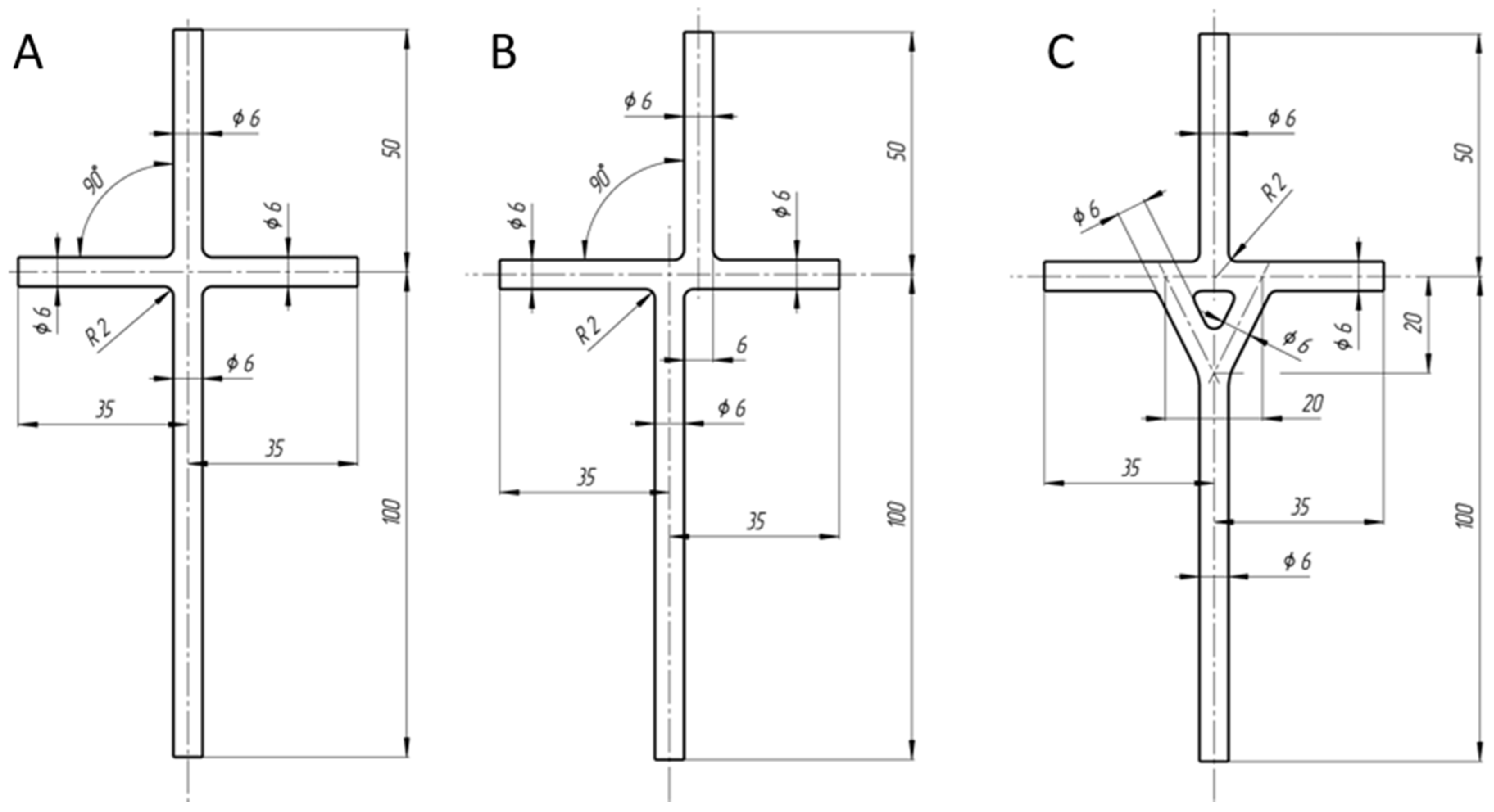
2.1. TCPC Models CFD

In this work we introduce flow simulation in a hydraulic system of the patient circulation with a Fontan connection. Herein, we show TCPC models in three various configurations: TCPC-1, TCPC-2, and TCPC-3, which simulate different options for connecting pulmonary arteries and vena cava. Geometric models with the major dimensions are shown in Figure 1. Figure 1A demonstrates the first TCPC-1 configuration. It represents a straight cross-shaped connection of vena cava and pulmonary arteries at angle of 90°. In this type of connection, a fluid flows from the superior and inferior vena cava towards each other, mixing together in the center, and then they are distributed between the pulmonary arteries. Figure 1B shows the configuration of TCPC-2 that differs from the first one by the 6 mm displacement of the vena cava relative to each other along the central line of the pulmonary arteries. The third TCPC-3 configuration is shown in Figure 1C and represents a so-called Y-connection. It is known that the diameter of the veins and arteries is not constant, but varies depending on the cardiac cycle state [11,12].

The diameters for all flow tubes were chosen equal to 6 mm, since this value is the most physiologically common for the group of five years old children.

2.2. TCPC Models Preparation

In order to perform bench tests, we manufactured three TCPC samples of various shapes. Their dimensions and geometry are shown in Figure 1. The finalized TCPC model is shown Figure 2C. The manufacturing process of the Fontan compound consists of several stages. ABS plastic blanks that repeat the geometry of the TCPCs were prepared via the Fortus 450mc (Stratasys Ltd., Rehovot, Israel) 3D printer. In order to connect TCPC to the hydraulic circuit, we used fittings with an inner diameter of 6 mm (Camozzi 2601 9-1/4, Camozzi Automation S.p.A., Brescia, Italy), which were installed in a transparent plexiglass base. To visualize the fluid flow, the layout is poured with Clear Flex 50 transparent polyurethane (Smooth-On, Inc., Macungie, PA, USA). After complete hardening, the product is placed in acetone that dissolves the 3D layout, forming a cavity inside the polyurethane form. The upper and lower surfaces of the model are completely transparent and allow us to visually observe the fluid flow profile.

The transparency of the side faces contributes to minimal loss of laser beam power when passing from the outer walls to the internal cavity of the TCPC model.

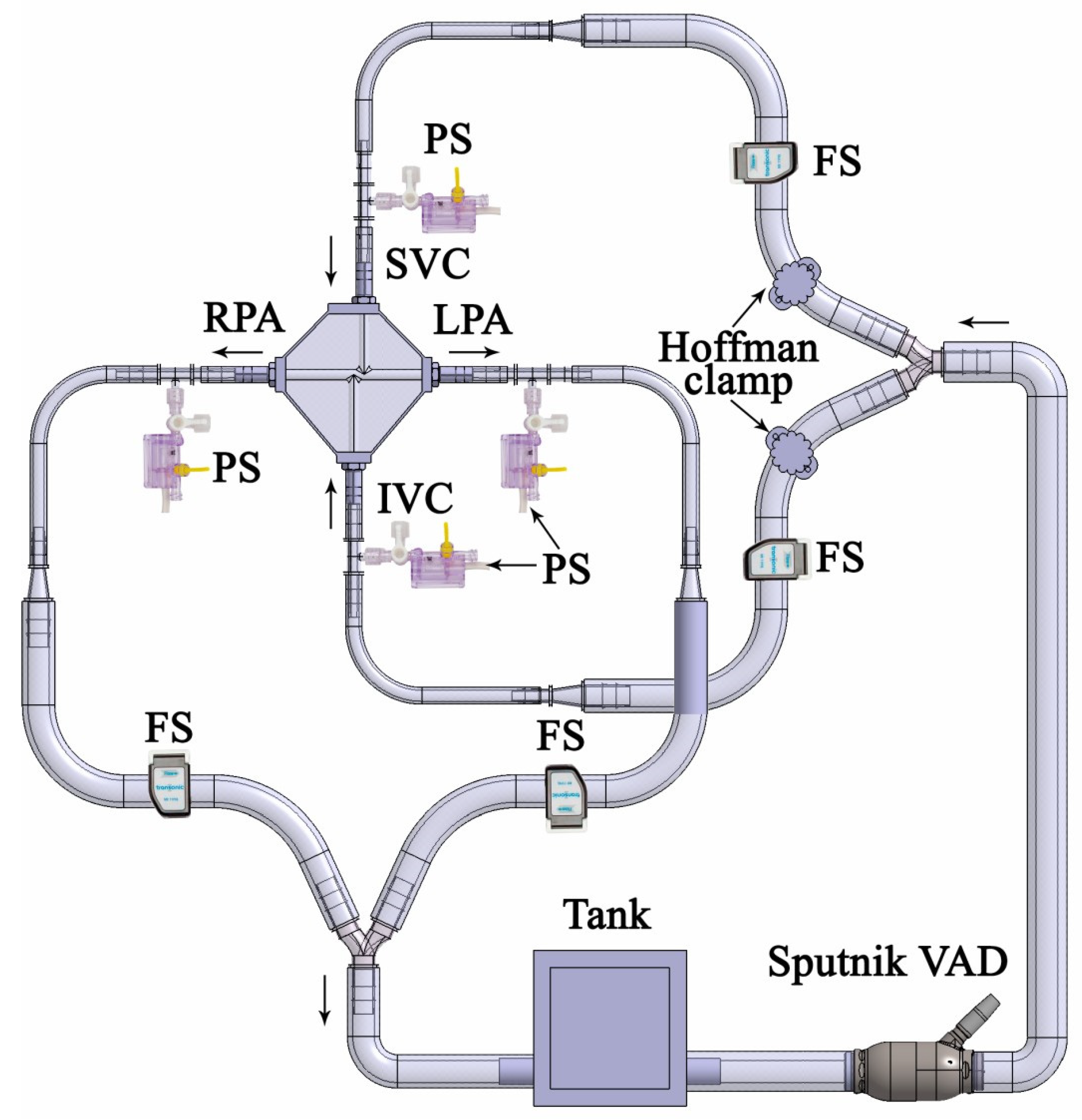
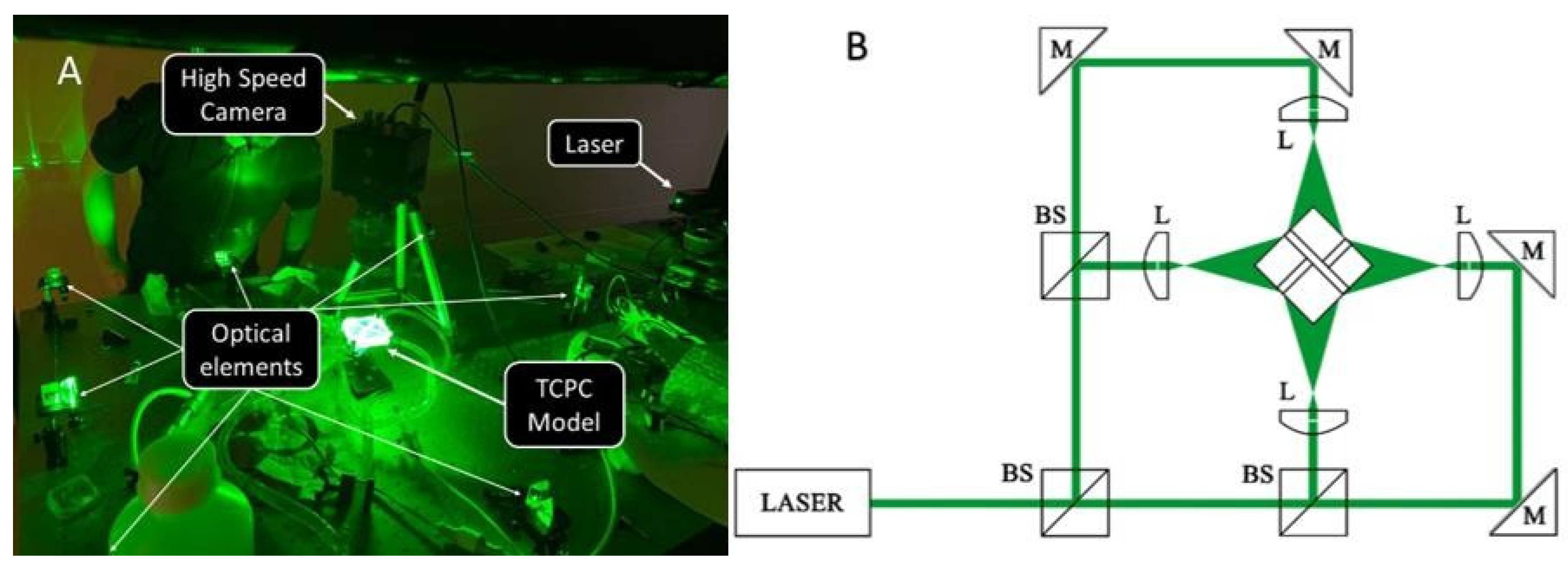
2.3. Mock Circulation Loop and Flow Visualization Setup

The hydraulic circuit of the bench is shown in Figure 3 and consists of a ventricular assist device (VAD) Sputnik pump [13], an open reservoir, and a Tygon transparent laboratory tube system (Tygon S3 E-3603, Saint-Gobain Performance Plastics, Courbevoie, France) with an internal diameter of ¼ and ½ inch. VAD “Sputnik” is a continuous type rotary blood pump. At a rotation speed of 6800 rpm, the pump provides the necessary range of fluid flow in the circuit from 0.5 to 3 L/min with 0.5 L/min step.

An aqueous solution of glycerol (57% distilled water and 43% glycerol by weight) was used as a model fluid. The working fluid density is 1104 kg/m³, the dynamic viscosity is 0.0035 Pa·s at 25 °C. The temperature of the used fluid corresponded to the ambient temperature. During all experiments, the temperature did not vary more than by 0.5 °C, which apparently does not have a significant effect on the working fluid viscosity.

Changes in fluid flow to LPA, RPA, IVC, and SVC were recorded using ultrasonic flow meters (ME-11PXL Clamp-on Tubing Flowsensors, Transonic System Inc., Ithaca, NY, USA), two modules for recording flow through tubes (TS410 Tubing Flow Module, Transonic System Inc., Ithaca, NY, USA), connected to a multichannel terminal (T402 Multi-Channel Research Console, Transonic System Inc., Ithaca, NY, USA). Hoffmann clamps were used to regulate the fluid flow through IVC and SVC in a proportion of 63%–37%. Four pressure port adapters were inserted into the hydraulic circuit of the bench for the connection of pressure sensors (TruWave disposable pressure transducers, Edwards Lifesciences Corporation, Al bay, CA, USA), which were connected directly at the inlet and outlet of the Fontan connection.

A particle image velocimetry (PIV) system was assembled to implement 2D fluid imaging. The motion path was recorded via the high-speed camera FASTCAM Mini AX 100 (Photron Limited, Tokyo, Japan), located perpendicularly to the laser beams. This camera allows us to get 4000 frames per second at a resolution of 1024 × 1024 pixels. The used lens was a Nikon 60 mm f/2.8G ED AF-S Micro-Nikkor (Nikon Corporation, Tokyo, Japan). The Fontan surface was illuminated by the DPSS laser (MGL-F- 532, Changchun New Industries Optoelectronics Technology Co., Ltd., Changchun, China) with a wavelength of 532 nm. The laser beam had a Gaussian profile shape. A long wavelength pass filter was installed in front of the camera lens to block the scattered laser radiation. The blood model fluid was seeded with neutral pink microspheres with a diameter of 20 µm (DiagPol Plain Fluorescent PMMA Particles, Creative Diagnostics, Upton, NY, USA). These particles luminesce in the yellow spectral range and are registered by the camera.

The optical scheme (Figure 4) consists of three beam splitters (NP 50:50 Beamsplitter Cube 400–700 nm, Thorlabs, Inc, Newton, NJ, USA), four dielectric mirrors (MRA20- E02-Right-Angle Prism Dielectric Mirror, 400–750 nm, Thorlabs, Inc, Newton, NJ, USA), and four cylindrical lenses (LJ1622L1-A Plano-Convex Cylindrical Lens, f = 25 mm, 350–700 nm, Thorlabs, Inc, Newton, NJ, USA). Cylindrical lenses are equidistant with respect to the TCPC model. In order to illuminate the full side surface of the model, the laser beam was divided into four similar beams. The diameter of the output laser beam was 2 mm.

The camera control, the data collection, and parameter settings were performed via the PFV software (Photron FASTCAM Viewer software, Photron, Tokyo, Japan).

To process images from a high-speed camera, the PIV lab toolbox [14] developed for MATLAB (MathWorks, Natick, MA, USA) was used.

A direct Fourier transform correlation with multiple passes and deforming windows was used for the data analysis. In most cases, this algorithm gives more accurate results. The algorithm analyzes the data in several stages: the first pass uses relatively large interrogation areas to calculate the displacement of image data reliably. The larger the interrogation areas, the better the signal-to-noise ratio, and the more robust the cross correlation. However, large interrogation areas will only give a very low vector resolution (“vectors per frame”). Therefore, in the following passes a smaller window size was used. The displacement information of the first pass is used to offset the interrogation areas in the second pass and so on (Figure 5). This procedure yields a high vector resolution, a high signal-to-noise ratio, and a high dynamic velocity range.

With the high-speed camera resolution and the height of the camera above the model of 200 mm, 1 pixel is equal to 60 microns of the real distance. Particles have a size of 1–2 pixels. The estimated maximum particle velocity can reach 2 m/s or 9 pixels per frame.

Thus, the minimum window of the first pass should be at least 18 pixels. For the faster algorithm operation, a window of 32 pixels was selected (Figure 5).

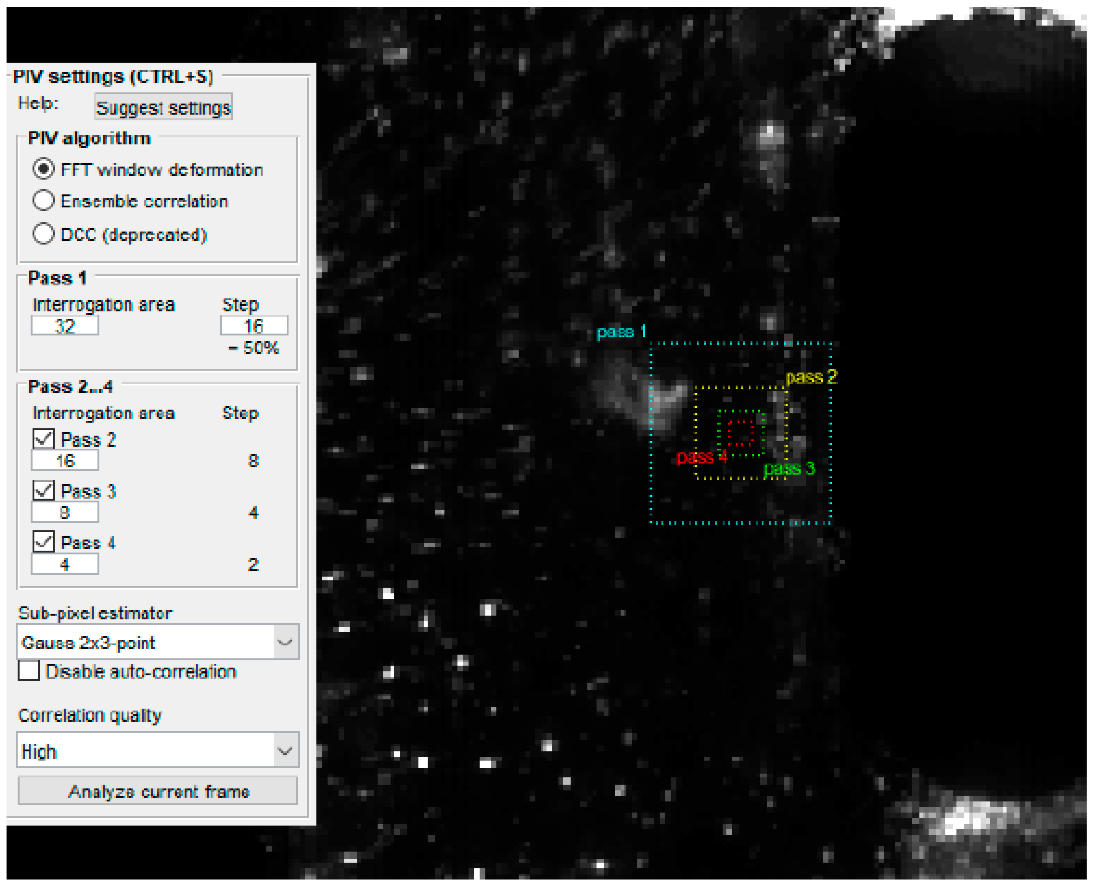
3. Measurement Techniques

CFD Study

Numerical simulation was carried out via the ANSYS 19.0 software package. The mesh preparation and generation was carried out via the Meshing module. Simulation of the fluid flow took place in the Fluent module. Based on three-dimensional models, three computational regions were obtained, consisting of unstructured grids with a total number of cells of about 250,000. The grids mainly consisted of the hexahedron families in the bulk and prismatic cells near the physical walls of the geometric model. The characteristic cell size lies in the range of 0.001–1 mm, depending on the local thickening of the grid. The parietal region consists of six layers of prismatic cells with the size of 0.005 mm or more.

Simulation of the flow process is based on the Navier–Stokes equations solutions. In this paper, we considered the stationary flow of a viscous fluid in a hydraulic system consisting of tube cross-sections located in a horizontal plane. Due to the action of viscous friction forces, the velocity of a fluid particle varies depending on its distance R to the axis of symmetry of each section of the hydraulic system. Due to the fact that the expected flow type in the tubes will be mainly laminar, the value determination of the Reynolds number dimensionless coefficient can be obtained via the equation:

$$Re=\frac{\rho VR}{\mu }$$

(1)

where, ρ is the fluid density, V is an average velocity, R is a tube radius, μ is a fluid viscosity.

In general, the fluid flow in this case is described by the Bernoulli equation, expressed in terms of pressure:

$${\frac{V}{2g}}^2+\frac{P}{\rho g}=H,$$

(2)

where P is a static pressure and H is the total head.

The flow simulation was based on the stationary condition, since the nonfunctional right ventricle is excluded for the circulation. For healthy patients from the age group of five years old children, the venous blood flow distribution between the superior and inferior vena cava is characterized by a ratio of 37%–63%, respectively. The cardiac output value is of 2.2 L/min [15]. The mean arterial pressure in the pulmonary arteries corresponds to 11 mmHg [16]. The efficiency of TCPCs was estimated via hydraulic power losses magnitude (see Equation (3)). Since there is no heat transfer, the hydraulic power losses magnitude is the only criterion for evaluating the efficiency of the hydraulic system. As a result, it is determined only by the flow part geometry. Hydraulic power losses are equal to the difference of total pressure at the inlet and outlet of the system. The total pressure is the sum of the average static and dynamic pressures in the cross-section of the tube. Hydraulic losses are determined by the difference in static pressures at the system inlet and outlet.

$$Power Loss=F_{IVC}·U_{IVC}·{\left(P_{static}+P_{dynamic}\right)}_{IVC}+F_{SVC}·U_{SVC}·{\left(P_{static}+P_{dynamic}\right)}_{SVC}-F_{LPA}·U_{LPA}·{\left(P_{static}+P_{dynamic}\right)}_{LPA}-F_{RPA}·U_{RPA}·{\left(P_{static}+P_{dynamic}\right)}_{RPA},$$

(3)

where $F$ is a cross-section area (${\mathrm{m}}^2$), $U$ is a mean value of velocity magnitude in a cross-section ($\mathrm{m}/\mathrm{s}$), $P_{static}$ is mean static pressure ($\mathrm{P}\mathrm{a}$) in a cross-section, $P_{dyn}=\frac{1}{2}\rho {\left|\overrightarrow{v}\right|}^2$ is mean dynamic pressure ($\mathrm{P}\mathrm{a}$) in a cross-section, and $\mathrm{Power}\mathrm{loss}$is power loss in the system (W). Subscripts IVC and SVC designate the inferior and superior vena cava, respectively. Subscripts LPA and RPA designate the left and right pulmonary artery, respectively.

Due to higher stability parameters of the implicit formulation, a converged steady-state solution was used. The convergence was carried out for the following parameters: velocity, pressure at the entrances, mass flow rates at the output, and was assessed using reference values which were below 0.001.

4. Characterization of Experimental Conditions

During the tests, the configuration of the experimental setup remained unchanged: the volume of fluid in the circuit was constant, the pressure sensors aligned with the atmosphere, there was ±0.5 °C temperature deviation from the room temperature, and the laser beams were converged at the same height.

At a rotation speed of 6800 rpm, the VAD Sputnik axial pump provided the necessary flow in the circuit. The flow sensors and pressure sensor readings were recorded for each test zone (SVC, IVC, RPA, LPA) at the flow rates of 0.5, 1, 1.5, 2, 2.2, 2.5, and 3 L/min. Observance of the necessary proportions when distributing the flow through the SVC and IVC was carried out using two Hoffmann clamps.

The total pressure is equal to the sum of the static and dynamic pressures in the measured area. In our case, due to technical limitations, it was not possible to measure the pressure directly at the inlet and outlet of the TCPC model. Pressure sensors were installed at a distance of 35 mm from the measurement location. In order to compensate losses in the additional section, the hydrodynamic losses dependence in the tube 𝑃_{𝑡𝑢𝑏𝑒} was determined and evaluated. These losses are due to friction within the moving fluid or along the tube walls. In addition, fluid viscosity has also an impact on the system dynamics and efficiency. It may likewise result from the physical elements used in the system such as the valve or the tube fittings. The aforementioned losses are classified as major (head) and minor losses.

$$P_{tube}={\displaystyle \sum }_1^k{P}_{Lmajo{r}_i}+{\displaystyle \sum }_1^k{P}_{Lmino{r}_i}$$

(4)

Major (head) loss is expressed via the Darcy–Weisbach equation:

$$P_{Lmajor}=f_D·\frac{L}{D}·\frac{{⟨\upsilon ⟩}^2}{2}·\rho$$

(5)

where $f_D$ is the Darcy friction factor, L is the pipe length (m), D is the hydraulic diameter of the pipe (m), $⟨\upsilon ⟩$ is the average water velocity (m/s), and ρ is the density of the fluid (kg/m³).

For the laminar flow, the following equation is used to calculate the friction factor

$$f_D=\frac{64}{Re}$$

(6)

where Re is the Reynolds number.

$P_{Lminor}$ is the minor losses caused by tube bends, fittings, and valves:

$$P_{Lminor}=K·\frac{{⟨\upsilon ⟩}^2}{2}·\rho$$

(7)

where K is the resistance coefficient.

Thus, Equation (3) was transformed. Calculation of power losses was carried out according to the following equation:

$$PowerLoss=Q_{IVC}·{(P_{static}+P_{dynamic}-P_{tube})}_{IVC}+Q_{SVC}·{(P_{static}+P_{dynamic}-P_{tube})}_{SVC}-Q_{LPA}·{(P_{static}+P_{dynamic}+P_{tube})}_{LPA}-Q_{RPA}·{(P_{static}+P_{dynamic}+P_{tube})}_{RPA} ,$$

(8)

where $Q_{IVC}, Q_{SVC}, Q_{LPA}, Q_{RPA}$ (m³/s) represent mean flow rates in IVC, SVC, LPA, and RPA, respectively.

5. Results

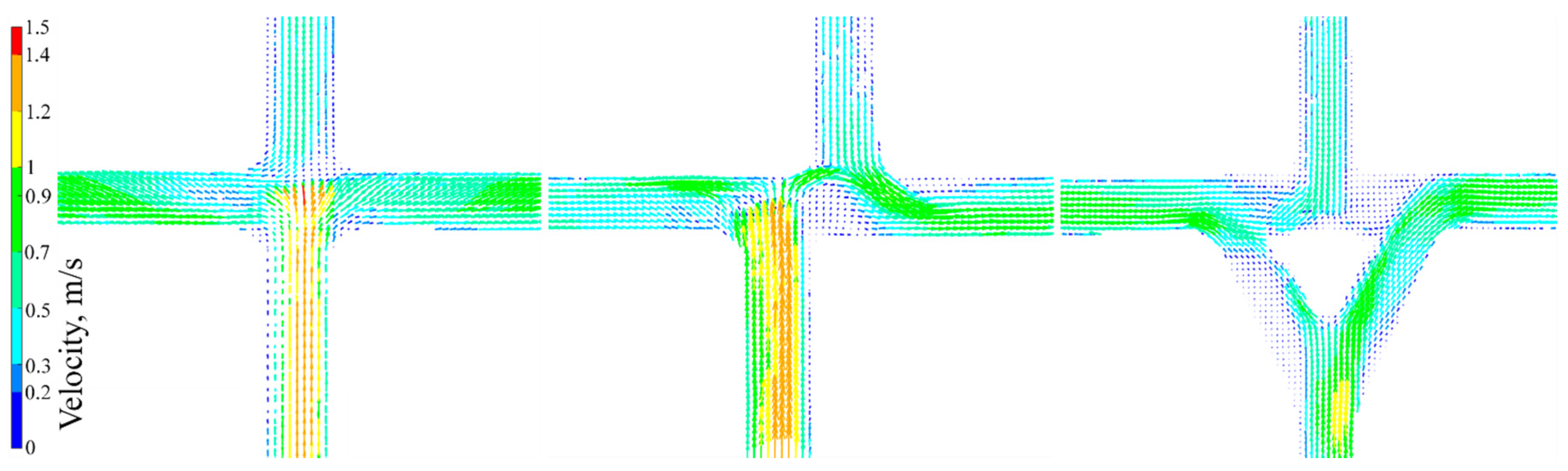
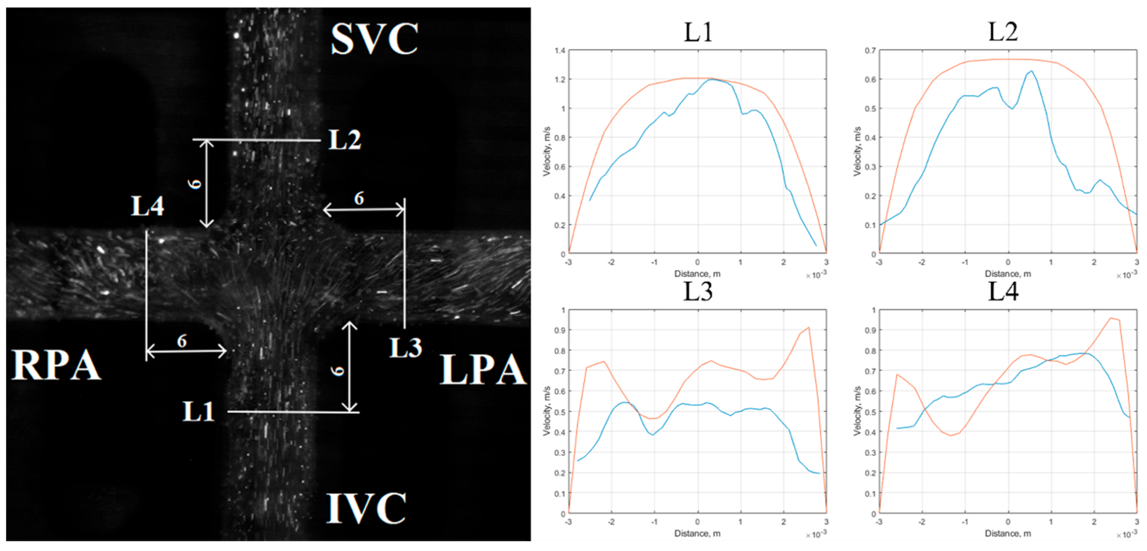
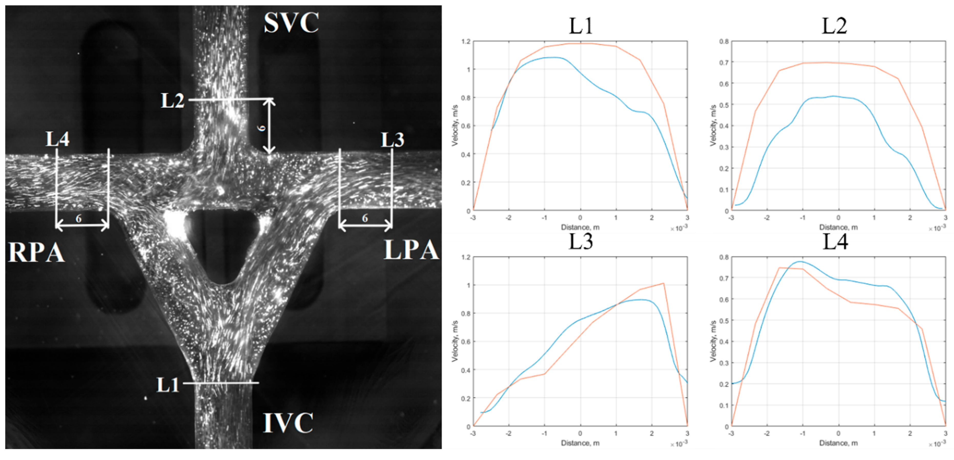
5.1. Velocity Field Results

For an operating point corresponding to a total flow rate of 2.2 L/min, the distributions of various flow parameters in the longitudinal section of TCPC systems are obtained. Figure 6 shows distribution of the flow velocity vector field obtained by the CFD simulation. The velocity vector field defines zones of local eddy flows. Figure 6A shows that the flow from the side of the inferior vena cava to the center inhibits the flow from the side of the superior vena cava, which inevitably leads to increased hydraulic losses. It can be seen in the Figure 6C diagram that the velocity value is less important, while the flow behavior is more uniform, due to this fact, the hydraulic losses of the TCPC system will be smaller. It should be noted that in TCPC-2 and TCPC-3 configurations, the stream is divided into two, practically not mixing with each other (Figure 6B,C).

The results of the experimentally obtained distribution of velocity vector field are shown in Figure 7. The flow profile in the TCPC-1 coincides with the CFD modeling results. The flow from the inferior vena cava increases up to the center of the TCPC. Abruptly it stops due to the oncoming pressure of the fluid and is evenly distributed in the LPA and RPA. The fluid moving through the IVC is interfered with the flow from the SVC and spun counterclockwise to the LPA and clockwise to the RPA. Further, the flow is stabilized. TCPC-3 has the lowest mean density of the velocity vector field. Thus, this connection has the smallest hydraulic loss.

Figure 8 shows the contour plot of the flow velocity modulus distribution obtained by the CFD simulation (A1–C1) and experimental data (A2–C2). The contour plot clearly shows areas where the flow reaches maximum speed and places where the speed values are minimal, this allows us to discuss the presence of the flow stagnation zones.

Figure 9 shows the contour plot of the static pressure distribution. The figure also shows the positions of the sections where the velocity profiles were built along a straight line perpendicular to the central axis of the tube. From the presented diagrams it can be observed that the greatest power losses take place in the TCPC-1 system (Figure 9A). It is shown that due to the incident flow of the inferior vena cava, the flow of the superior vena cava in the center is strongly inhibited and a region of increased pressure appears. In TCPC-2 (Figure 9B), the flow behavior from the inferior vena cava is similar to the case described above. It should be noted that the flow hits the wall of the pulmonary artery, as a result local pressure increases due to a decrease in the flow rate. In contrast, in the TCPC-3 system (Figure 9C), the pressure distribution is more uniform.

In order to get a complete picture of the fluid flow in the TCPC models, data on the velocity distribution in the cross-sections was obtained. From the presented data (Figure 10) it can be observed that the experimentally obtained data is in good agreement with the CFD simulation data. In some cases, even repeating the curve shape. Cross-section L2 belongs to SVC and to a less degree corresponds to CFD simulation data. In this section, the flow is compressed closer to the center. From section L2, it becomes obvious that at the SVC entrance of the model there is an additional local hydraulic resistance due to ≈1 mm constriction of the pipe section.

In TCPC-2 (Figure 11), flows are more evenly divided. However, there is one stagnation zone. Experimental data correlate with the CFD simulation data. This can be seen on cross-sections L3 and L4, which repeat the distribution shape. The distribution shape at cross-section L1 is different: the flow (blue line) is shifted towards the LPA due to the unevenness of the tubes at the entrance to the model. Cross-section L2 also reflects the presence of an additional local hydraulic resistance.

Figure 12 shows the velocity modulus distribution data for TCPC-3. The experimentally obtained fluid flow in TCPC-3 perfectly correlates with CFD simulation data. The only exception is for cross-section L2 where the flow velocity modulus (blue line) is about 10–15% lower.

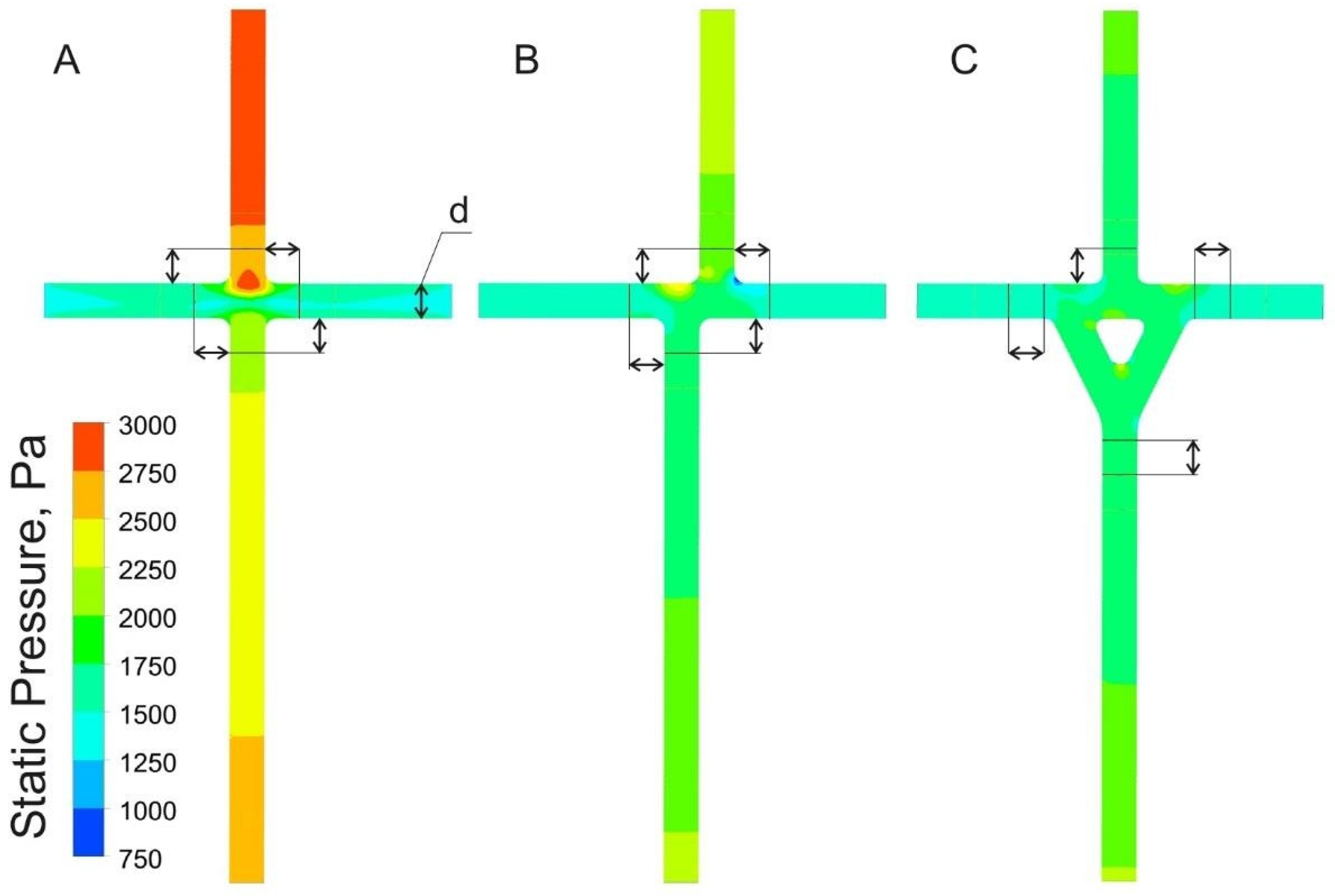
5.2. Hydraulic Results

Figure 13 shows the power loss of various TCPC systems as a function of the flow rate at the operating point. The minimum power loss corresponds to TCPC-3 connection, where at the operating point of 2.2 L/min losses are equal to 0.04 W. The maximum power loss is 0.087 W for TCPC-1 (CFD). The difference between the experimental results and the simulation results at the operating point does not exceed 0.014 W. Curve shapes for each of the TCPC models are similar.

6. Discussion

Treating patients with right ventricular dysfunction is a complex clinical task. These patients are at a constant risk of complications such as systemic venous hypertension, thromboembolism, and congestive heart failure [17], therefore, the hemodynamics restoration of the cardiovascular system (CVS) for patients with a single-ventricular heart is an important scientific and practical task. In order to restore the hemodynamics of CVS, it is necessary (I) to increase the efficiency of passive blood transfer to CVS, and (II) to provide mechanical support for circulation. The combination of these two approaches is designed to relieve the single-ventricular heart and reduce the risk of heart failure. In this work, the first (I) approach is considered.

Computer simulation of the flow in various configurations of TCPC allows one to predict the flow behavior with high accuracy from the distribution of the vector velocity field point of view. This is confirmed by the experiment. Due to this fact, it is possible to clearly observe low flow rates and recirculation zones. In TCPC-1 and TCPC-2 configurations, the blood lines intersect at right angles, which leads to a sharp increase in the velocity value in the region where fluid from IVC and SVC flows towards each other. In case of TCPC-2, flows are distributed more smoothly, however the presence of a direct connection leads to the appearance of a recirculation flow when passing from the IVC and SVC. The graphs showing the comparison of velocity profiles for TCPC-1 and TCPC-2 models demonstrate that in cross-sections closer to the flow connection zone, differences in the behavior of velocity profiles are observed. We assume that this is due to the more chaotic behavior of the incoming flows. Moreover, at a distance of two diameters from the walls along the pulmonary axis, the profiles acquire a characteristic parabolic shape, indicating the formation of a laminar type of flow. In case of TCPC-3, due to the smoother connections of the blood lines, the flow behavior significantly differs from the other two configurations. A significant decrease in flow rate was noted during the transition of the flow from IVC to LPA and RPA. This is due to an increase in the total cross-sectional area of the channel due to its bifurcation. The coincidence of the experimental graphs of the velocity profiles with the graphs obtained as a result of the simulation confirms that the flow behavior in all sections of the hydraulic system is smoother. As a result, TCPC-3 configuration has higher energy characteristics and lower hydraulic resistance of the system. Considering the hydraulic system of TCPC in terms of hydraulic losses, TCPC-3 also has a significant advantage at a flow rate of 2.5 L/min compared to TCPC-1. As a drawback of TCPC-3 system, one can note the lack of symmetry of the velocity field during flow separation at the center of the joint. As a result of this, a decrease in the flow rate is observed in one channel, which may adversely affect the process of thrombosis, but this requires a more detailed study. Additionally, this separation of the flow leads to the fact that SVC and IVC flows practically do not mix with each other. This observation also requires additional research.

The energy efficiency of Fontan circulation was described elsewhere [6]. There were discussions on the limitations of energy loss calculations with various assumptions, e.g., steady flow conditions as performed in this study. CFD analysis method of hemodynamic characteristics is used in the majority of studies. In present work, we used both CFD and studies on physical TCPC models, that allows to compare theoretical and practical models. As opposed to previous studies, velocity distribution in the cross-sections of TCPC models were obtained.

It was shown that the TCPC geometry has a great influence on the hemodynamics [18,19]. For more accurate results, the vessel size will be patient-specified with increased 16–18 mm diameter conduits for 2–3 years old children [20]. In our case, TCPC geometry is idealized and rigid. Pulmonary arteries and vena cava sizes were chosen based on studies on geometry and dimensions of the pulmonary artery bifurcation in children and adolescents [11,12].

The present work is a first step in the complex validation and a basement for future studies with patient-specific TCPCs, pulsatile flow, and mechanical circulatory support. As a result, obtained data can be an ideal tool for the following in-depth investigation of the powered Fontan connection.

Limitation

An absence of the pulsating flow should be considered as a limitation of the presented study. The pulsating flow will be investigated in the following work on the different TCPC configurations under the VAD support.

Another limitation is a use of rigid tube systems instead of flexible tube systems. It should be noted that the compliance and elasticity of the vessel walls were shown to have significant impact on the function of Fontan circulation [21].

7. Conclusions

Based on the obtained results, TCPC-3 configuration with the pump supported circulation can be considered as the best out of three configurations. This configuration allows to (i) potentially minimize the risk of thromboembolism, (ii) reduce the load of the only functional ventricle and decrease the risk of chronic venous hypertension, and (iii) significantly reduce the power loss of the system for Fontan patients. Moreover, these results nicely correlate with energetics of blood flow in previously performed simulation of Fontan circulation. In all sections of the geometric model, we can observe a laminar flow model, which indicates the physiological nature of the flow. Inspired by these results, we plan to perform further experiments using a pediatric rotary blood pump. Thus, we will be able to obtain TCPC model results for patients with an auxiliary blood pump connected. The blood flow will be simulated, and profile of the flow will be evaluated, as a result, we will investigate pump influence on hemolysis in detail. As for now, this study already indicates what type of TCPC system should be used for the improvement of the Fontan patient’s life until a donor heart is available for transplantation.

References

1. Khairy, P.; Poirier, N.; Mercier, L.-A. Univentricular Heart. Circulation 2007, 115, 800–812. [Google Scholar] [CrossRef] [PubMed] [Green Version]
2. De Leval, M.R.; Deanfield, J.E. Four decades of Fontan palliation. Nat. Rev. Cardiol. 2010, 7, 520–527. [Google Scholar] [CrossRef] [PubMed]
3. Mack, E.; Untaroiu, A. Hemodynamics Characteristics of a Four-Way Right-Atrium Bypass Connector. J. Fluids Eng. 2018, 140, 121106. [Google Scholar] [CrossRef]
4. Jagani, J.; Untaroiu, A. A Study of TCPC-Stent Conjunction for Cavopulmonary Assist in Fontan Patients with Right Ventricular Dysfunction. In Proceedings of the American Society of Mechanical Engineers, Phoenix, AZ, USA, 11–17 November; Volume 7, p. V007T09A093.
5. Marsden, A.L.; Bernstein, A.J.; Reddy, V.M.; Shadden, S.C.; Spilker, R.L.; Chan, F.P.; Taylor, C.A.; Feinstein, J.A. Evaluation of a novel Y-shaped extracardiac Fontan baffle using computational fluid dynamics. J. Thorac. Cardiovasc. Surg. 2009, 137, 394–403. [Google Scholar] [CrossRef] [PubMed] [Green Version]
6. Rijnberg, F.M.; Hazekamp, M.G.; Wentzel, J.J.; de Koning, P.J.H.; Westenberg, J.J.M.; Jongbloed, M.R.M.; Blom, N.A.; Roest, A.A.W. Energetics of Blood Flow in Cardiovascular Disease. Circulation 2018, 137, 2393–2407. [Google Scholar] [CrossRef] [PubMed] [Green Version]
7. Ni, M.W.; Prather, R.O.; Rodriguez, G.; Quinn, R.; Divo, E.; Fogel, M.; Kassab, A.J.; DeCampli, W.M. Computational Investigation of a Self-Powered Fontan Circulation. Cardiovasc. Eng. Technol. 2018, 9, 202–216. [Google Scholar] [CrossRef] [PubMed]
8. Migliavacca, F.; Dubini, G.; Bove, E.L.; de Leval, M.R. Computational Fluid Dynamics Simulations in Realistic 3-D Geometries of the Total Cavopulmonary Anastomosis: The Influence of the Inferior Caval Anastomosis. J. Biomech. Eng. 2003, 125, 805–813. [Google Scholar] [CrossRef] [PubMed]
9. Soerensen, D.D.; Pekkan, K.; de Zélicourt, D.; Sharma, S.; Kanter, K.; Fogel, M.; Yoganathan, A.P. Introduction of a New Optimized Total Cavopulmonary Connection. Ann. Thorac. Surg. 2007, 83, 2182–2190. [Google Scholar] [CrossRef] [PubMed]
10. Telyshev, D.; Denisov, M.; Markov, A.; Fresiello, L.; Verbelen, T.; Selishchev, S. Energetics of blood flow in Fontan circulation under VAD support. Artif. Organs 2020, 44, 50–57. [Google Scholar] [CrossRef] [PubMed] [Green Version]
11. Kutty, S.; Li, L.; Hasan, R.; Peng, Q.; Rangamani, S.; Danford, D.A. Systemic Venous Diameters, Collapsibility Indices, and Right Atrial Measurements in Normal Pediatric Subjects. J. Am. Soc. Echocardiogr. 2014, 27, 155–162. [Google Scholar] [CrossRef] [PubMed]
12. Knobel, Z.; Kellenberger, C.J.; Kaiser, T.; Albisetti, M.; Bergsträsser, E.; Valsangiacomo Buechel, E.R. Geometry and dimensions of the pulmonary artery bifurcation in children and adolescents: Assessment in vivo by contrast-enhanced MR-angiography. Int. J. Cardiovasc. Imaging 2011, 27, 385–396. [Google Scholar] [CrossRef] [PubMed]
13. Telyshev, D.; Denisov, M.; Pugovkin, A.; Selishchev, S.; Nesterenko, I. The Progress in the Novel Pediatric Rotary Blood Pump Sputnik Development. Artif. Organs 2018, 42, 432–443. [Google Scholar] [CrossRef] [PubMed]
14. Thielicke, W.; Stamhuis, E.J. PIVlab—Towards User-friendly, Affordable and Accurate Digital Particle Image Velocimetry in MATLAB. J. Open Res. Softw. 2014, 2. [Google Scholar] [CrossRef] [Green Version]
15. Cheng, C.P.; Herfkens, R.J.; Taylor, C.A.; Feinstein, J.A. Proximal pulmonary artery blood flow characteristics in healthy subjects measured in an upright posture using MRI: The effects of exercise and age. J. Magn. Reson. Imaging 2005, 21, 752–758. [Google Scholar] [CrossRef] [PubMed]
16. Rowe, R.; Eden, F.R.C.P. The normal pulmonary arteriel pressures in the first year of life. J. Pediatr. 1957, 51, 1–4. [Google Scholar] [CrossRef]
17. Throckmorton, A.L.; Chopski, S.G. Pediatric Circulatory Support: Current Strategies and Future Directions. Biventricular and Univentricular Mechanical Assistance. ASAIO J. 2008, 54, 491–497. [Google Scholar] [CrossRef] [PubMed]
18. Tang, E.; Restrepo, M.; Haggerty, C.M.; Mirabella, L.; Bethel, J.; Whitehead, K.K.; Fogel, M.A.; Yoganathan, A.P. Geometric Characterization of Patient-Specific Total Cavopulmonary Connections and its Relationship to Hemodynamics. JACC Cardiovasc. Imaging 2014, 7, 215–224. [Google Scholar] [CrossRef] [PubMed] [Green Version]
19. Dasi, L.P.; KrishnankuttyRema, R.; Kitajima, H.D.; Pekkan, K.; Sundareswaran, K.S.; Fogel, M.; Sharma, S.; Whitehead, K.; Kanter, K.; Yoganathan, A.P. Fontan hemodynamics: Importance of pulmonary artery diameter. J. Thorac. Cardiovasc. Surg. 2009, 137, 560–564. [Google Scholar] [CrossRef] [PubMed] [Green Version]
20. Itatani, K.; Miyaji, K.; Tomoyasu, T.; Nakahata, Y.; Ohara, K.; Takamoto, S.; Ishii, M. Optimal Conduit Size of the Extracardiac Fontan Operation Based on Energy Loss and Flow Stagnation. Ann. Thorac. Surg. 2009, 88, 565–573. [Google Scholar] [CrossRef] [PubMed]
21. Kilner, P.J. Valveless pump models that laid a false but fortuitous trail on the way towards the total cavopulmonary connection. Cardiol. Young 2005, 15, 74–79. [Google Scholar] [CrossRef] [PubMed]
Figure 1. Schematic of three different geometry configurations of total cavopulmonary connections (TCPCs) chosen for the research in this work. (A) Simple direct joint, where the inferior vena cava (IVC) and superior vena cava (SVC) are coaxially arranged (model is shown with dimensions). (B) Compound where the IVC and SVC are shifted by the distance of a single diameter (6 mm). This type of compound is often used in TCPC surgery. (C) More complex type of curvilinear connection, where IVC is divided into two vessels and connected to the left pulmonary artery (LPA) and right pulmonary artery (RPA) at an angle, directing the flow along a smoother trajectory.
Applsci 10 06910 g001
Figure 2. Manufacturing process of transparent TCPC model: (A) 3D blank, (B) transparent plexiglass base with installed fittings and 3D blank, (C) finalized TCPC model given with dimensions.
Applsci 10 06910 g002
Figure 3. Mock circulation loop, where constant flow generated by Sputnik pump. Changes in pressure and flow in LPA, RPA, IVC, and SVC were detected by FSs (flow sensor) and PSs (pressure sensor). The flow direction is shown by arrows.
Applsci 10 06910 g003
Figure 4. (A) Photo of the experimental bench and (B) optical scheme of the experimental bench, where BS is beam splitters, M—mirrors, L—cylindrical lens.
Applsci 10 06910 g004
Figure 5. Windows of each pass in the TCPC-3 image with particle image velocimetry (PIV) settings.
Applsci 10 06910 g005
Figure 6. Distribution of the flow velocity vector field obtained by the computational fluid dynamics (CFD) simulation. Velocity values for the color gradient are given in the sub picture. Flows from inferior and superior vena cava bump into each other that increases the hydraulic losses. Flows in TCPC-2 and TCPC-3 are divided into two parts, effectively decreasing hydraulic losses.
Applsci 10 06910 g006
Figure 7. Distribution of the flow velocity vector field obtained by experimental data. Flow profiles are similar to CFD results. TCPC-3 has the lowest mean density of the velocity.
Applsci 10 06910 g007
Figure 8. The contour plot of the flow velocity modulus distribution obtained by CFD simulation (A1,B1,C1) and experimental data (A2,B2,C2). The contour plot shows areas where the flow reaches maximum speed and places where the speed values are minimal.
Applsci 10 06910 g008
Figure 9. The contour plot of the static pressure distribution. Pressure values for the color gradient are given in the sub picture. The greatest power loss is in TCPC-1. The flow in TCPC-2 hits the wall of the pulmonary artery, as a result local pressure increases due to a decrease in the flow rate. TCPC-3 pressure distribution is steady and well-distributed.
Applsci 10 06910 g009
Figure 10. Velocity modulus distribution in various sections for TCPC-1: red line—CFD modeling, blue line—experimental data. L1, L3, and L4 repeating the curve shape for both methods. In cross-section L2 flow is compressed closer to the center due to the design features of internal cavity of SVC.
Applsci 10 06910 g010
Figure 11. Velocity modulus distribution in various sections for TCPC-2: red line—CFD modeling, blue line—experimental data. L3 and L4 repeat the distribution shape. At L1 (blue line) it is shifted towards the LPA. L2 (blue line) reflects the presence of an additional local hydraulic resistance.
Applsci 10 06910 g011
Figure 12. Velocity modulus distribution in various sections for TCPC-3: red line—CFD modeling, blue line—experimental data. TCPC-3 has the most correspondence between experimental and CFD results.
Applsci 10 06910 g012
Figure 13. Comparison of power loss of TCPC systems for experimental setup (dashed line) and computational fluid dynamics simulation (solid line). Yellow, green, and red lines correspond to TCPC 1–3 models, respectively.
Applsci 10 06910 g013