Abstract
A reliable quantification of greenhouse gas emissions is a basis for the development of adequate mitigation measures. Protocols for emission measurements and data analysis approaches to extrapolate to accurate annual emission values are a substantial prerequisite in this context. We systematically analyzed the benefit of supervised machine learning methods to project methane emissions from a naturally ventilated cattle building with a concrete solid floor and manure scraper located in Northern Germany. We took into account approximately 40 weeks of hourly emission measurements and compared model predictions using eight regression approaches, 27 different sampling scenarios and four measures of model accuracy. Data normalization was applied based on median and quartile range. A correlation analysis was performed to evaluate the influence of individual features. This indicated only a very weak linear relation between the methane emission and features that are typically used to predict methane emission values of naturally ventilated barns. It further highlighted the added value of including day-time and squared ambient temperature as features. The error of the predicted emission values was in general below 10%. The results from Gaussian processes, ordinary multilinear regression and neural networks were least robust. More robust results were obtained with multilinear regression with regularization, support vector machines and particularly the ensemble methods gradient boosting and random forest. The latter had the added value to be rather insensitive against the normalization procedure. In the case of multilinear regression, also the removal of not significantly linearly related variables (i.e., keeping only the day-time component) led to robust modeling results. We concluded that measurement protocols with 7 days and six measurement periods can be considered sufficient to model methane emissions from the dairy barn with solid floor with manure scraper, particularly when periods are distributed over the year with a preference for transition periods. Features should be normalized according to median and quartile range and must be carefully selected depending on the modeling approach.
1. Introduction
Climate change is one of the great challenges of our century. In order to develop adequate mitigation measures, greenhouse gas emissions in all economic sectors, including agriculture, need to be soundly quantified [1,2,3]. In the context of livestock husbandry, methane is a substance of particular importance [4,5,6,7]. It emerges during decomposition processes in manure and during ruminants digestion and makes up about 44% of the sector’s greenhouse gas emissions [8]. The Food and Agricultural Organization (FAO) of the United Nations estimated that dairy cattle husbandry contributes 20% of the total greenhouse gas emissions from the livestock sector. One important issue in this context is that the emission dynamics from the digestive system of the ruminants and from the manure are different. Emissions from manure are expected to increase exponentially when the ambient temperature is above approximately 15 C, while emissions from the digestive system follow rather a parabolic curve in dependence on the temperature with minimal emissions from lactating dairy cattle at ambient temperatures around 10 C [9,10]. Particularly when housed in barns with solid floor and manure scraper (i.e., no significant manure storage inside the building), a substantial part of the methane emissions from dairy cattle husbandry is associated with the fermentation activity in the rumen, where approximately 92% of the gas leaves the body via eructation and breath [11].
Although there are mechanistic models that predict the emission of individual cattle, the evaluation of methane emissions on the housing level is challenging [12,13,14,15]. Besides temperature, animal and farm-specific parameters (e.g., feed composition and feeding time) as well as local air flows affect the overall emissions. The latter is particularly challenging as dairy cattle (if not on pastures) are commonly kept in naturally ventilated buildings where indoor air flow is governed by constantly changing inflow conditions. A continuous measurement of the methane emissions from such buildings is, however, barely possible since the area of inlets and outlets is large and the openings are dynamically changing their role as inlet or outlet in response to the varying ambient conditions. This, besides technical challenges, results in high expense for monitoring the inlet and outlet openings and a preference for intermittent measurement strategies [16].
In many studies, air exchange rates and gaseous emissions are estimated by balancing gas (particularly CO) inside and outside the building on a few days distributed over the year. It is recommended to include hot, cold, and moderate days [17]. Annual emission values are derived from those measurements by using weighted averages or regression equations based on easy accessible explanatory variables (e.g., ambient temperature, inflow wind speed, herd composition, floor type, etc.). In the past, this procedure was frequently applied to model ammonia emissions and extrapolate to annual ammonia emission factors, where in most cases a multilinear model was fitted to the logarithmized emission values [18,19].
With more and more data being compiled the interest in testing machine learning approaches in the context of emission modeling continues to increase with first promising results [20,21]. It has been recently observed for ammonia emissions from a naturally ventilated barn that the procedure of fitting multilinear models is rather sensitive to outliers in the measurements while the robustness of the prediction can be improved by applying advanced data science approaches (particularly ensemble methods) [21]. Uncertainties of around 20% have been found with current sampling strategies even with machine learning in that study. The additional level of complexity due to the two different indoor sources of methane and the non-monotonic influence of temperature may even further decrease the accuracy of empirical modeling of methane emissions from barns with ruminants when applying standard multilinear models.
Here, we investigated the following two hypotheses related to the estimation of methane emission factors from cattle barns with solid floor with manure scraper: (1) The accuracy of the model prediction can be improved if the squared temperature value is included as an additional feature in the modeling process, while considering a logarithmic function as in the case of ammonia is not useful, because preceding studies have indicated that emissions from the digestive system show rather a parabolic dependence on the temperature. (2) Empirical modeling with multilinear approaches is less robust (i.e., less reliable in making correct predictions under small perturbations in the training data) than machine learning approaches to predict aggregated emission values, where ensemble methods are the most robust and time efficient machine learning approaches to model methane emissions.
Therefore, our study compares and evaluates the accuracy and robustness of different machine learning approaches when projecting emission values of a dairy cattle barn using different training datasets that reflect commonly applied sampling strategies in the course of a year and include standard features (i.e., easily measurable on-farm). By that we want to provide a guideline for the selection of temporal sampling strategy and empirical modeling approach for future studies to derive methane emission factors.
2. Materials and Methods
2.1. Data Collection
In the following subsections, we describe where, when and how the dataset from a naturally ventilated dairy barn, as used in this study, was collected.
2.1.1. Measurement Site
We considered a dairy cattle building in Mecklenburg-Western Pomerania, Germany, close to the Baltic Sea [21]. The naturally ventilated building had dimensions 96.15 m × 34.20 m × 10.7 m (length × width × gable height). One of its 4.2 m high, open side walls faced the prevailing wind direction. Each gable wall had four doors and one gate with adjustable curtains. There was a 0.5 m gap in the roof.
Within the measurement period, there were four climate-controlled ceiling fans and two automatic scrapers to clean the solid concrete floor every 90 min. On average 355 dairy cattle with 682 kg body mass and 39 kg milk yield per day were kept in loose housing with cubicles with a 0.2 m deep straw and chalk bedding. Cows went out for milking in four groups three times a day for approximately 45 min (starting approximately at 06:00 a.m., 02:00 p.m. and 10:00 p.m.). Around 06:45 a.m. and 10:30 a.m., a total mixed ration consisting of soy (24%), oil-seed rape (19%), maize (24%), rye (23%), and lupins (10%) was provided.
2.1.2. Measurement Setup
Gas samples were collected with 10 Teflon sampling lines with an inner diameter of 6 mm and an orifice every 8–10 m. One line was below the ridge, the rest at a height of around 3.2 m. Four lines were outside, the other lines inside the building, all with a distance of at least 4 m to the walls [22]. Lines were sampled one by one for 10 min each with one of two high resolution Fourier Transform Infrared (FTIR) spectrometer (Gasmet CX4000, Gasmet Technologies Inc., Karlsruhe, Germany) monitoring carbon dioxide and methane concentrations from 1 November 2016 until 30 August 2017. In consequence, per sample line 7276 hourly values (approximately 10 months) of gas concentrations were available. We obtained the values of ambient air temperature at a distance of 5 m from the building and estimated average flow conditions (wind speed and direction) from the values measured with an anemometer at the roof of the building. Amount, mass and yield of the dairy cattle were obtained as daily herd averages from the farm administration.
We estimated indoor methane () and carbon dioxide () concentrations by averaging all indoor sample lines for each hour. The outdoor sample line with the lowest CO concentration at each hour was used to obtain CO and CH concentrations in the incoming air. We applied the CO mass balancing method (Equation (1)) to calculate ventilation rates.
Here Q is the ventilation rate, i.e., the volume flow, in , N is the amount of cows and is the difference of the carbon dioxide concentration of the air indoor and outdoor in . production per cow ( in ) was derived from cow mass, milk yield, days in milk and ambient air temperature [23]. Outdoor air temperature was used as a proxy for the indoor temperature, since the offset between both is usually small and temperature sensitivity of the production model is also low [24]. The indoor–outdoor methane concentration difference in was multiplied with the ventilation rate Q and scaled with the cow mass to calculate normalized methane emissions as illustrated in Equation (2).
Here one LU is the body mass equivalent of 500 kg, N is the amount of cows in the building and m is their average mass in kg.
2.2. Regression Analysis
We tested several regression approaches to extrapolate the dynamics of methane emissions over the seasons. A Pearson correlation analysis was performed to assess the linear relation of standard features (i.e., the explanatory variables) with the observed methane emission. From the regression we obtained the hourly emission values, i.e., the response variables, as functions of the explanatory variables time, temperature, squared temperature, wind speed and direction, where time and wind direction were treated as cyclic variables (resulting in a total of nine features). The time was encoded by sine and cosine transformed features with periods of 24 h respectively 365 days. That way, the day-time (hour of the day) and the year-time (day of the year) components were decoupled. The wind direction was sine and cosine encoded with a period of 360. We further considered a model using only the sine and cosine transformed feature of day-time as explanatory variables. Predicted emissions were evaluated against the observed emissions averaged over the entire 10 months measuring period.
2.2.1. Machine Learning Methods
We applied gradient boosting (GradBoost) and random forests (RandFor), both ensemble methods; ordinary (multi-) linear regression (LinReg) and linear regression with regularization, known as ridge regression (Ridge); a shallow neural network with one hidden layer (fixAnn) and more advanced neural network architectures, where the number of hidden layers and nodes per layer are optimized (ANN); support vector machines (SVM) and Gaussian processes (GausProc), implemented in Python 3 using the library Scikit-learn 0.22.1 [25].
The ensemble methods we used are based on decision trees [26] and in contrast to many other machine learning approaches, they do not require hyperparameter tuning. While random forests average over the predictions of a set of trees that are based on different subsets of features [27], gradient boosting improves an initial regression tree sequentially, following a gradient descent approach [28,29].
The (multi-) linear regression and the ridge regression we used, both minimize the least square function. The difference between these methods is an additional regularization term in the ridge regression case [30], which leads to a tunable hyperparameter. This so-called regularization strength was tuned by a randomized search using the function RandomizedSearchCV of Scikit-learn [25].
Artificial neural networks [31,32,33,34] consisting of one input layer and one, two, four or eight fully connected hidden layers, as well as a single output layer, that is a single real value in the case of regression, were considered here. The number of nodes varied between 8, 16, 32 and 64, but was the same within each hidden layer. Hyperparameters (i.e., number of hidden layers and number of nodes per layer) were tuned using GridSearchCV of Scikit-learn [25]. As activation function a rectified linear unit (ReLU) was employed [35]. Weights were tuned by backpropagation of the loss function, while the model was trained with the Adam optimizer (adaptive moment estimation) [36]. We used the MLPRegressor-function (multi-layer perceptron regression) from scikit-learn [25]. Furthermore, we studied the shallow neural network architecture (one hidden layer with four nodes) suggested by Wang et al. for modeling ammonia emissions of cattle barns with natural ventilation [20].
The principle of support vector machines, initially designed for classification problems [37], was transferred to regression tasks [38] in the implementation of support vector regression in scikit-learn [25]. We used the RBF kernel (radial basis function) and tuned the hyperparameters C (regularization parameter) and (kernel coefficient) with RandomizedSearchCV [25].
Finally, we examined Bayesian function approximation methods (Gaussian Processes) [39], using the GaussianProcessRegressor of scikit-learn [25]. We deployed a Matern kernel function, which generates nonlinear function approximations [39]. During model training, the hyperparameters (kernel parameters and observation noise) were automatically tuned on a log-marginal-likelihood basis.
Further details on the mentioned methods can be found in the preceding study by Hempel et al. on ammonia emission modeling with machine learning [21].
Feature normalization is advisable before applying any machine learning procedure if the magnitude of the values is expected to be considerably different (e.g., when as in our case temperature and squared temperature are considered as features). The performance of some machine learning approaches, particularly ANNs, can be considerably affected by the feature normalization where normalization based on the median is considered superior over a standard z-score normalization [40]. Here we used the RobustScaler from sklearn [25] which removes the median and scales the data according to the quantile range.
2.2.2. Sampling of Training Data and Cross-Validation
Under practical considerations, up to six measurement periods with not more than 14 days are realistic to estimate annual emission values, since due to the high investment costs of suitable measurement devices repeated short-term measurements are preferred over continuous measurements.
We randomly picked three, four, and six periods (each with a length of 1, 7 and 14 days) out of our approximately 10 months of hourly data, in order to investigate the effect of different measurement scenarios (i.e., frequency, length and timing of measurements in the course of a year) on the model predictions (compare the procedure in [21]). The intervals were selected under the constraint of including predetermined seasons, namely summer (June to August, with night temperature around 11 C and day temperature around 21 C), winter (January and February, with night temperature around −2 C and day temperature around 3 C) and transition (March to May and September to December, with night temperature around 3 C and day temperature around 10 C). An overview of the 27 measurement scenarios is given in Figure 1. For each of the scenarios 30 random realizations were considered.
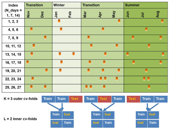
Figure 1.
Sketch of the 27 survey schemes, studied in the evaluation of the regression models in a nested cross-validation setup for hyperparameter optimization and error estimation. Indices refer to the 27 scenarios with associated lengths of the measurement periods. The allocation of the selected measurement periods to the individual seasons (transition, summer and winter) is marked in the figure, where the distribution within the seasons is random (with 30 realizations per scenario). The cross-validation scheme is sketched exemplary for three measurement periods. Confer also [21].
This subset of data was used to train and evaluate the model in a nested cross-validation setup, where we estimated the extrapolation error in an outer K-folds cross-validation loop and, if needed, optimized hyperparameters in an inner L-folds cross-validation loop. The splitting into “Test” (i.e., validation data in outer loop), “Eval” (i.e., validation data in inner loop) and “Train” set (i.e., training data in inner loop) was done using GroupShuffleSplit from scikit-learn [25]. The best hyperparameter configuration found in the inner validation loop was used to re-train the model in the outer training set. Finally, since we had approximately 40 weeks of continuous measurement data available, we also evaluated the model on all of the data not included in the train and test sets of the outer cross validation to obtain the extrapolation error.
In each scenario, one measurement period was used as evaluation dataset and one measurement period was used as test dataset. Since the number and length of measurement periods varied from scenario to scenario, the proportion of training, validation and test cases also varied. For each realization and each iteration of the cross-validation loop, 0.3% to 5% of the whole dataset was used for learning hyperparmeters and another 0.3% to 5% for validating the hyperparmeter choice. Approximately 0.7% to 25% of the whole dataset was used for re-training in the outer validation loop each time (i.e., to calculate the training error), while 0.3% to 5% were used for testing in the outer loop (i.e., to calculate the test error). The remaining 99% to 70% of the data were used to estimate the extrapolation error.
2.2.3. Evaluation Measures
The ranking of different modeling approaches can not be expected to be the same when different sets of training data and different evaluation criteria are used [21]. In order to investigate if the same trends as in the case of ammonia modeling can be observed when modeling methane emissions with machine learning, we considered the same scenarios for temporal sampling (Figure 1).
For each scenario, we calculated the mean and the standard deviation of the projected emission values, when using 30 random combinations of measurement periods for model training (whilst taking into account the scenario constraints). In addition, we calculated the quartiles and interquartile ranges for each scenario based on these 30 realizations. The R value (coefficient of determination) as well as the root mean squared error (RMSE) and the mean absolute error (MAE) of the projected emissions relative to the observed hourly emission values were compared. Those measures evaluate how well the emission dynamics are reproduced by the models. In addition, we present the total absolute error (TAE; i.e., the absolute difference between the average 10-month emission value in the observations and the model predictions).
2.2.4. Graphical Representations
Using Matplotlib, version 3.1.3 [41] we created confidence and box plots to visualize the results. In the confidence plots the one sigma interval, i.e., (where is the mean value and is the standard deviation), is shown. In the box plots the interquartile ranges were considered, where is the upper quartile limit and is the lower quartile limit. The upper whisker in the box plot extend to the last value less than and the lower extend to the first value larger than , where . The horizontal orange line inside the boxes hightlights the median, whereas outliers (i.e., data beyond the whiskers) were plotted as circles.
3. Results
We calculated the mean observed emission = 11.6 g h LU by averaging over the monitored 10 months.
3.1. Feature Selection
By comparing the Pearson correlation coefficients of the different features with the target emission values and the logarithm of the emissions we found that considering the logarithm of the emissions (as it is the common procedure for example in the case of ammonia) did not considerably improve predictions when modeling methane emissions. From Table 1 it can be seen that the correlation in most cases was very low and even decreased when considering the logarithm. On the other hand, we found that using the feature instead of T considerably increased the obtained correlation coefficient. The highest absolute value of the correlation coefficient, i.e., the highest expected predictive performance of individual features, was obtained from the day-time components followed by the squared temperature. The obtained correlation coefficients highlighted that for the studied phenomena there was only very little linear relationship. The existence of a non-linear relationship in the case of day-time and temperature can be seen from the scatter plots in Figure 2.

Table 1.
Pearson correlation coefficients between all features and the methane emission E, respectively the logarithm of the emission ln(E), as target. Here, T refers to the ambient air temperature close to the building. Wind speed and wind direction were monitored by an anemometer on the roof.
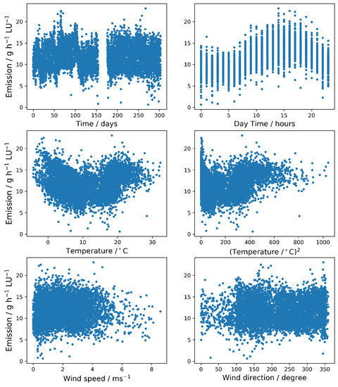
Figure 2.
Scatter plots between the target size (emission) and the input features (year-time, day-time, temperature, squared temperature, wind speed and wind direction).
3.2. Prediction Accuracy
In general, it is advisable in regression analysis to focus on those input variable that are highly linearly correlated with the output variable. As shown before, in the case of methane emissions from our naturally ventilated cattle building under consideration, none of the routinely monitored features fulfilled this criterion. Nevertheless, there are apparently non-linear relations that justify the use of those features in the modeling process. We considered the predictions of the average emission values obtained by multiple models.
In row 1 of Figure 3, we present the results obtained by gradient boosting and random forest. The two ensemble methods produced very similar results with a very accurate and robust prediction of the 10-month average emission value. Less than 10% relative error were obtained even for scenarios where only three times 24 h were used for model training. Linear regression with regularization (Ridge, 2nd row left) and without regularization (LinReg, 2nd row right) with scenarios with three to four measurement periods resulted in very different emission values. Linear regression without regularization exhibited larger deviations from the actually measured value and particularly a larger variability (partly with relative errors around 25%). The results with scenarios with six measurement periods, were more comparable to the outcome of the ensemble methods. The projected emission values obtained with an artificial neural network with hyperparameter tuning (ANN, left) and a simple neural network with one hidden layer and four nodes (fixAnn, right) are depicted in the third row. The more complex network resulted in general in projections that were closer to the experimental value. In addition, the variance was smaller than obtained from fixANN. However, the complex ANN generally tended to slightly overestimate the emission values. The deviations from the actually measured mean were typically larger than observed with the machine learning methods in row 1 and 2. The results of the Gaussian process model (GaussProc, right) and the support vector machine (SVM, left) are compared in the last row. The SVM predictions were similar to the results with Ridge. With the Gaussian process the variability was larger and almost all mean values were below the experimental value.
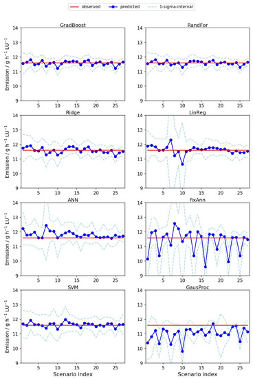
Figure 3.
Predictions of methane emissions [] averaged over the 10 month measuring period with eight regression methods. The mean over the predictions, based on 30 random realizations of each of the 27 scenarios (as depicted in Figure 1), is highlighted in blue. The associated one-sigma intervals are indicated by the light blue dashed lines. Here, all methods used the features: T (i.e., outdoor temperature), , wind speed, wind direction, time and day-time, scaled with the RobustScaler from Scikit-learn [25]. For comparison, red horizontal lines highlight the mean observed emission ( = 11.6 g h LU).
Next, we compared the model projections when considering all features versus using only a selection of features for modeling, since the correlation analysis indicated that the linear relation between the methane emission and the considered features is usually very week. In consequence, taking into account all features might reduce the predictive accuracy, particularly in the case of multilinear regression. The results of this empirical study are summarized examplarily for GradBoost, LinReg and Rigde in Table 2. We observed that in the case of multilinear regression (i.e., LinReg and Ridge) neglecting all but the sine and cosine of the day-time indeed improved the prediction accuracy. A similar behavior as with the linear regression was observed using the ANN approach (results not shown). The predictions of the methane emissions for the different scenarios that were obtained with the multilinear regression in that reduced model setup can be seen in Figure 4. For other methods, such as GradBoost, including all features usually produced slighly better results.
Table 2.
Averaged emission (Emiss.), mean absolute extrapolation error (MAE), total absolute error (TAE), and mean absolute test error (test err.) averaged over all scenarios. Emission, MAE, TAE and test error are provided in g h LU. Note: The averaged experimental emission was 11.596 g h LU. The smallest errors are highlighted in red.
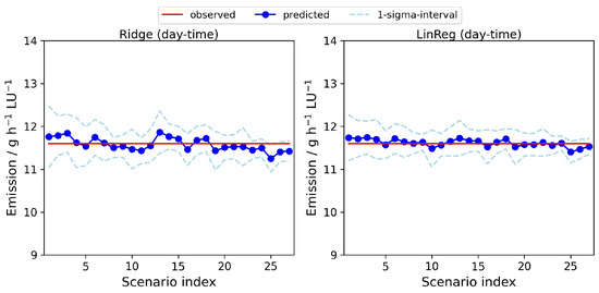
Figure 4.
Predictions of methane emissions averaged over the 10 month measuring period with two regression methods and only the sine and cosine transformed day-time as input features. The mean over the predictions based on 30 random realizations of each of the 27 scenarios (as depicted in Figure 1) is marked in blue. The associated one-sigma intervals are indicated by the light blue dashed lines. The red horizontal lines highlight the mean observed emission ( = 11.6 g h LU).
In summary, the worst results were obtained with fixAnn followed by GausProc. LinReg and ANN performed better for scenarios with six measurement periods, but variability for scenarios with fewer measurement periods was also high, if all features were taken into account for modeling. Including only the sine and cosine transformed day-time feature, the prediction accuracy of LinReg considerably increased for scenarios with fewer measurement periods. The results from Ridge and SVM were comparable to LinReg and ANN for six measurement periods and all features included. The variability for scenarios with fewer measurement periods was lower in this setup. The variability of the Ridge results could be further decreased by neglecting less linearly correlated features. GradBoost and RandFor achieved the least variable results in the setup with all features combined with on average small deviations from the actual value. The results of the ensemble methods were comparable to those of LinReg and Ridge with reduced number of input features, but more robust against the selection of features.
3.3. Evaluation Criterion and Temporal Sampling
Next we compare a selection of the presented methods in more detail. The selection was mainly based on the performance of the methods summarized in Figure 3 and Figure 4, where GradBoost, LinReg (day-time) and SVM were among the best performing methods. With RandFor and Ridge (day-time) we also obtained very good results for the predicted 10-months average emission value, but results were almost identical to GradBoost and LinReg (day-time), while the latter were faster. Thus, we selected only GradBoost and LinReg (day-time) for the detailed investigation. As a forth method we considered ANN in the detailed investigation since this method is a frequently used modern machine learning technique in the context of emission modeling in contemporary literature [20,42,43,44,45]. The comparison of the mentioned four methods in terms of train, test and extrapolation error confirmed the ranking of these methods found before (see Figure 5 and Figure 6). GradBoost and LinReg (day-time) achieved in general the lowest error values. SVM performed slightly worse in terms of the test and extrapolation error, particularly in scenarios with three and four measurement periods. The train error was comparable amongst GradBoost and SVM, but larger with LinReg (day-time). ANN resulted in the largest errors amongst the four methods. In general, the results for the test error deviated more among the methods than for the train and extrapolation error. For larger training sets the different types of errors were more similar than for smaller training sets.
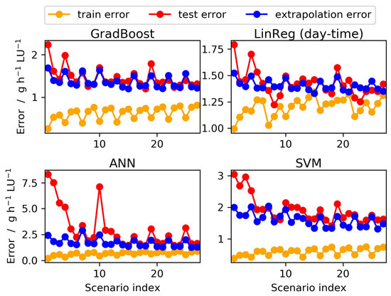
Figure 5.
Mean absolute errors [] for four distinct regression methods (where LinReg used only the sine and cosine transformed day-time feature and the other three methods used all features). In each case, the error was determined on three different datasets: The data that were used for learning (train error depicted in orange), the data that were used for model testing in the cross-validation (test error depicted in red) and the data that were not used in the cross-validation (extrapolation error depicted in blue). All error values were averaged over 30 realizations of data selection, which fulfill the scenario constraints. Please note that the y-axes in the subplots have different scaling.
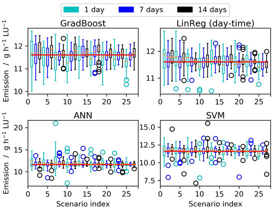
Figure 6.
Averaged emissions [] predicted by gradient boosting, multilinear regression with reduced number of input features, a hyperparameter-tuned artificial neural network and support vector regression. The box plots show the mean values and the variabilities based on 30 random realizations of each scenario, where the associated length of the measurement period in the scenario is indicated by the colors cyan (1 day), blue (7 days) and black (14 days). For comparison the mean observed emission value (11.6 , calculated from the full experimental dataset) is indicated by a red line. Please note that the y-axes have different scaling.
The box plots for the same selection of methods indicate that the variability of the projected values in general decreased if larger training datasets were used, while the trend with regard to the average value was less pronounced (see Figure 6). However, in many cases, in scenarios with 7 and 14 days the average value was closer to the actual 10-month average than in scenarios with only 1 day.
Furthermore, GradBoost exhibited clearly the least outliers among all realizations. Therefore, GradBoost was selected to further evaluate the effect of sampling frequency and duration on the model predictions on the basis of different accuracy measures. Figure 7 indicates that scenarios resulting in very accurate average emission values did not necessarily result in low extrapolation errors. Among the scenarios with reasonably low MAE and at the same time small deviation between the projected and the measured average emission value were the scenarios 20, 21, 23, 24, 26 and 27. All of those were scenarios with 6 time 7 days (in case of scenarios 20, 23 and 26) or 14 days (in the other cases). Moreover, the mentioned scenarios had a strong focus on transition periods in the training datasets.
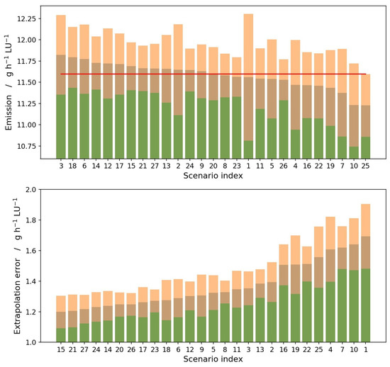
Figure 7.
Ranking of the explored scenarios: In the upper diagram, scenario indices are sorted based on the mean predicted emission values, starting with the largest value. In the lower diagram, scenario indices are sorted based on the mean absolute extrapolation errors (MAE), starting with the smallest error. All means were calculated over 30 realizations per scenario and are represented by the border between brown and orange bars. The width of the one-sigma interval is indicated by the orange and brown bars. The red line in the upper panel corresponds to experimental emissions averaged over the 10 month measuring period (11.6 ).
This can be also seen in Table 3. The three best performing models in terms of MAE, RMSE and R were all scenarios with six times 14 days. The lowest TAE (i.e., the best prediction of the 10-month average emission value), on the other hand, was obtained in a scenario with six times 7 days, followed by scenarios with four times 14 days and four times 7 days. Most of the best performing methods focused on data from transition periods. Particularly, winter measurements were under-represented in the best performing scenarios.
Table 3.
Mean absolute error (MAE in g h LU), root mean squared error (RMSE in g h LU), coefficient of determination (R, dimensionless) and total absolute error (TAE in g h LU), calculated for gradient boosting on data disjoint from train and test sets. In addition, the total average error relative to the average observed emission value (%TAE in%) is provided. Red color highlights the best three results and bold face the worst results. The three lowest error values of MAE, RMSE and R resulted from the scenarios 15, 21 and 27, while scenarios 8, 9 and 20 produced the lowest TAE.
4. Discussion
In the following, we discuss the role of the individual features, the temporal sampling and the evaluation criterion in the process of empirical modeling of methane emissions as well as the potential added value and ranking of the different common machine learning approaches.
4.1. Role of Individual Features
Our correlation analysis indicated that particularly the day-time components can explain a substantial part of the variability in the emission of methane from the naturally ventilated barn with concrete floor considered in this study. The key role of the day-time components is likely closely related to the fact that methane emissions are essentially determined by the feed intake [4]. In consequence, the timing of feed supply and milking is a central clock for the circadian rhythm of methane emissions. In husbandry systems with feed supply in the early morning, at midday and in the afternoon three peaks were reported in literature [46]. For feeding systems with feed supply in the morning and the afternoon a bimodal distribution of methane over the day has been reported [4]. In contrast, for systems with feed supply in the early and the late morning, as on the farm in our study, there is typically one pronounced maximum of methane emission over the day [10,47]. These diurnal rhythms that are discussed in the literature do not only explain the high absolute value of the correlation coefficient between the day-time components and the methane emission, but also why the correlation in our case is negative. With feed supply on the farm in our study in the early and late morning the emission maximum is observed in the late afternoon [10]. This timing of the maximum coincides neither with the maximum of the sine nor the maximum of the cosine, but is phase shifted relative to the trigonometric functions. In consequence, negative correlation coefficients were obtained.
The observed diurnal rhythms in methane emissions can, however, not only be explained by feed supply as even on pasture, where feed is continuously available, diurnal patterns of the methane emission have been found [48]. Other possibly influencing variables besides feed supply are the change between light and darkness and the ambient temperature, both affecting the general activity level of the animals. Preceeding studies have indicated, that methane emissions notably depend on the ambient temperature. Considering large temperature intervals, an increase of the methane emission towards both edges of the thermoneutral zone (i.e., the temperature interval where most of the metabolizable energy can be used for production) was reported in literature [10]. This immediately suggests that a consideration of the ambient temperature as a linear variable alone is not enough, which is also indicated by the low correlation coefficient in our analysis. In consequence, the consideration of the squared temperature as a feature is valuable for the modeling of the emissions, which is indicated by the correlation coefficient that is almost twice as high for squared temperature compared to the temperature itself. It has also been found that, after an increase of the methane emissions under mild to moderate heat stress conditions, under severe heat stress methane emissions go down again [49]. However, under the typical climatical conditions in our study region squared temperature can be expected to be sufficient to model the influence of ambient temperature on the methane emission.
High wind speed can reduce heat load and thus modulate the emission pattern induced by the ambient temperature [50]. Moreover, high wind speed is associated with a larger volume flow from the naturally ventilated building and can thus result in higher emissions in general as less of the produced gas is trapped inside the building. Our correlation analysis, however, indicated that these effects play a minor role. An even lower correlation was found between methane emissions and wind direction. This can be explained by the fact that the latter basically effects the local wind speed and local air exchange inside the building [51].
The low correlations of the methane emissions with the year time components can be explained by the fact that the time of the year only indirectly affects the methane emissions (e.g., by varying temperature, feed quality, milk yield or cow mass) [4,10,52].
Finally, in contrast to other pollutant emissions (such as ammonia), the linkage to the logarithm of the methane emission is lower than to the methane emission itself. This can be explained by the fact that, while emissions from manure basically follow Arrhenius law (i.e., exponential increase of the emissions with increasing temperature), direct emissions from the digestive system exhibit different dynamics. In our study the barn was equipped with solid concrete floor that was scraped every 90 min so that manure-borne methanogenic conversion processes were neglectable in the overall emission process. In consequence, the monitored methane emissions must be governed by the digestive processes which do not show an exponential increase with temperature [10].
4.2. Added Value and Ranking of Machine Learning Approaches
Our study indicated that with the mentioned selection of features, most modeling approaches, even the simple multilinear regression, in general agree acceptably well with the aggregated emission value. Although individual realizations of the scenarios (i.e., selections of training data) led to over- and underestimation, in most cases the relative deviation from the actual mean emission value was below 10%. This is considerably better than the ±20% range reported for ammonia emission modeling in preceding studies [21,53]. Only with the simple neural network geometry (fixAnn), the Gaussian Process (GausProc) and some scenarios with the standard multilinear regression (LinReg) a substantial variability of the estimated emission values among the realizations of the scenarios was reported in the current study. This means that it was unlikely to select a suboptimal training period. This is in contrast to the findings in a preceding study on ammonia emission with a similar modeling setup [21]. The main differences between the preceding and the current study were (i) the slightly different choice of features due to the different dependency of the emission dynamics of the two gases on temperature (Section 4.1) and (ii) the data normalization approach. In contrast to the preceding study, here we applied a normalization based on median and quantile range. The latter can reduce the influence of outliers of individual features during the model training. Thus, it can make model projection more robust, since many classifiers use Euclidean distance to evaluated the suitability of selected parameter values. If one feature has a broader range of values, the final value of the distance will be influenced more strongly by this particular feature. Tests of different normalization approaches (results not shown), with the methane emission related dataset used in this study, indicated that the effect of data normalization is particularly relevant for the neural network approaches ANN and fixAnn as well as for GausProc. However, moderate effects were observed also for support vector machines (SVM), and linear regession with and without regularization (Ridge and LinReg), while the ensemble methods (GradBoost and RandFor) were almost insensitive to data normalization. This represents a clear added value of the usage of ensemble methods for the empirical modeling of methane emissions, which can be expected also for the modeling of other gaseous emissions.
In addition, as found also in the before mentioned study for ammonia, ensemble methods provided one of the most robust projections of the methane emissions in our study (see Section 3.2). We observed that GradBoost and RandFor with reduced measurement setups (scenarios 1–12) achieved similar accuracy as LinReg with extended measurement setups (scenarios 13–27) with six measurement periods, when all input features were used for modeling. In addition, with six measurement periods the ensemble methods were even more reliable in terms of reduced variability of the model projection among the 30 realizations. If only the strongest linearly correlated input features were taken into account in the modeling, LinReg also achieved good results even with reduced measurement setups. In consequence, particularly when only three or four measurement periods are available, a very careful selection of input features or the use of ensemble methods for projecting methane emission values is advisable.
4.3. Role of Temporal Sampling and Evaluation Criterion
In terms of TAE the scenario 20, a scenario using six measurement periods with 7 days was ranked highest, followed by scenarios 8 and 9. The latter two were scenarios with only four measurement periods, which, however, achieved only moderate model errors. Except for scenarios 1 and 13 which were highly ranked in terms of TAE but not in terms of model error, there was no scenario with only 1 day of measurements per period among the best performing scenarios. This was similar to the findings for the projection of ammonia emissions in the before mentioned study [21]. The ammonia study reported acceptable results with scenarios 25 and 22 in terms of TAE but not in terms of model error. In our current study on methane, however, these two scenarios were rather low ranked in terms of TAE and model error. Moreover, while the study for ammonia reported no scenario with only three measurement periods among the best ranked ones, here we found that scenario 1 and 2 reached acceptable results in term of the TAE, but low quality in terms of model error. In the preceding study on ammonia only the scenario 12 reached good performance in terms of both TAE and model error. In the current study on methane this scenario, however, was ranked only on an intermediate place.
All of this indicates that while the recommendation of six times 7 days of measurements seems to be rather general, in specific situations and setups also smaller training datasets can achieve good modeling results for gaseous emissions from cattle barns with regularly scraped solid concrete floor. The latter is in accordance with the recommendations of the VERA (i.e., Verification of Environmental Technologies for Agricultural Production) protocol for housing systems which also recommends a minimum of six measurement periods distributed over the year with at least 1 day of measurements [17].
Moreover, in accordance with the study on ammonia, we found that most of the best performing methods focused on training data from transition periods and measurement periods with a duration of at least 7 days. Among the best performing scenarios winter measurements were particularly underrepresented while transition periods should be preferred. This is likely related to the fact that the emission dynamics during transition times represent conditions close to the annual average while during winter and summer more extreme emission value can be expected. Our results further support the previous findings that scenarios with 7 days and 14 days result in a comparable model performance. In consequence, measurement protocols with 7 days can be considered sufficient, particularly in setups with six measurement periods distributed over the year with a preference for transition periods with moderate temperatures.
5. Conclusions
Correlation analysis indicated that in the case of a naturally ventilated cattle building with regularly scraped solid concrete floor particularly the day-time components, and to a minor degree the squared ambient temperature and the ambient temperature, can explain the variability in the emission of methane. In addition, wind speed, wind direction and the year time components modulated the emission pattern. In contrast to other pollutant emissions, such as ammonia, the linkage to the logarithm of the methane emission was lower than to the methane emission itself. Thus, the methane emission value itself should be considered as output variable in the modeling process. It should be noted that the relevant features might be different in husbandry systems where the manure is not almost immediately removed.
Our initial assumption that the additional level of complexity due to the two different indoor sources of methane and the non-monotonic influence of temperature may further decrease the accuracy of empirical modeling of methane emissions compared to those of ammonia when applying standard multilinear models could not be verified. With the above mentioned selection of features and a suitable data normalization strategy, most modeling approaches, even the simple multilinear regression, reached in general acceptable agreement with the aggregated emission value, where in most cases the relative deviation was below 10% (confirming Hypothesis 1). In the case of multilinear regression, the results were even better when only the day-time components were included as input features. The simple neural network without hyperparameter tuning obtained the worst results followed by the Gaussian processes. Multilinear regression and neural networks with hyperparameter tuning performed better for scenarios with six measurement periods, but also exhibited high variability for scenarios with fewer measurement periods when all features were included. The results from multilinear regression with regularization (all features included) and from support vector machines were comparable to the former mentioned in the case of six measurement periods, but showed less variability for scenarios with fewer measurement periods. The ensemble methods gradient boosting and random forest resulted in on average small deviations from the actual value combined with the least variable results and can thus be considered very robust in terms of the selection of individual training data within a temporal sampling scenario. Moreover, they had the added value to be rather insensitive against the normalization procedure and the inclusion of nonlinearly related input features.
While a recommendation of six times 7 days of measurements seems to be rather general applicable, in specific situations and setups also smaller training datasets were able to achieve good modeling results for methane emissions. We observed that, when using all input features, the ensemble methods with reduced measurement setups (three to four measurement periods) achieved similar accuracy as the multilinear regression with extended measurement setups with six measurement periods (confirming Hypothesis 2). We found that most of the best performing methods focused on training data from transition periods. Our results further support previous findings that scenarios with 7 and 14 days result in a comparable model performance. In consequence, measurement protocols with 7 days and six measurement periods can be considered sufficient, particularly when periods were distributed over the year with a preference for transition periods and features were normalized according to median and quartile range. Either gradient boosting should be used for modeling or only input features that are strongly linearly related to the methane emission should be used for modeling.
Nonetheless, with a coefficient of determination of about 66% even the best models in this study could not explain about one third of the variability in the emission data. Considering interactions of the features could be an option to slightly increase model accuracy. Predictions might be improved further, if other input features that are more closely and directly related to the emission process (e.g., exact timing, amount and composition of feed intake, bacterial composition and conditions in the rumen, etc.) will be included. However, those features are usually barely measurable under on-farm conditions.
Author Contributions
Conceptualization, S.H., J.A., N.L., D.W., D.J. and T.A.; methodology, J.A., N.L. and S.H.; software, J.A., N.L. and D.W.; validation, S.H., J.A., D.W., D.J., T.A. and N.L.; formal analysis, J.A. and S.H.; investigation, D.J., D.W., S.H. and J.A.; resources, N.L. and T.A.; data curation, D.W., D.J. and S.H.; writing—original draft preparation, S.H. and J.A.; writing—review and editing, S.H., J.A., N.L., D.W., D.J. and T.A.; visualization, J.A.; supervision, T.A., N.L. and S.H. All authors have read and agree to the published version of the manuscript.
Funding
This research was partially funded by the German Research Foundation (Deutsche Forschungsgemeinschaft), grant number LA 3270/1-1. The publication of this article was funded by the Open Access Fund of the Leibniz Association.
Acknowledgments
We acknowledge the support of ATB’s technicians Ulrich Stollberg and Andreas Reinhard in the course of the measurements. We further thank the Landesforschungsanstalt für Landwirtschaft und Fischerei Mecklenburg-Vorpommern (LFA-MV), particularly Anke Römer, Bernd Losand, and Christiane Hansen, as well as the staff of Gut Dummerstorf for providing comprehensive data on animals and climatic conditions.
Conflicts of Interest
The authors declare no conflict of interest. The funders had no role in the design of the study; in the collection, analyses, or interpretation of data; in the writing of the manuscript, or in the decision to publish the results.
Abbreviations
The following abbreviations were used in this manuscript:
| PTFE | polytetrafluoroethylene (i.e., teflon) |
| FTIR | Fourier Transform Infrared |
| LU | Livestock Unit (500 kg body mass equivalent) |
| GradBoost | Gradient Boosting |
| RandForest | Random Forest |
| Ridge | Regularized Multilinear Regression |
| LinReg | Ordinary Multilinear Regression |
| ANN | Artificial Neural Network |
| fixAnn | Artificial Neural Network with fixed number of hidden layers and nodes |
| GaussProc | Gaussian Process |
| SVM | Support Vector Machine |
| MAE | Mean Absolute Error |
| RMSE | Root Mean Square Error |
| TAE | Total Absolute Error |
References
- Sutton, M.A.; Bleeker, A.; Howard, C.; Erisman, J.; Abrol, Y.; Bekunda, M.; Datta, A.; Davidson, E.; de Vries, W.; Oenema, O.; et al. Our Nutrient World. The Challenge to Produce More Food & Energy with Less Pollution; Technical Report; Centre for Ecology & Hydrology: Edinburgh, UK, 2013. [Google Scholar]
- Masson-Delmotte, V.; Zhai, P.; Pörtner, H.O.; Roberts, D.; Skea, J.; Shukla, P.R.; Pirani, A.; Moufouma-Okia, W.; Péan, C.; Pidcock, R.; et al. Global Warming of 1.5 °C. In An IPCC Special Report on the Impacts of Global Warming of 1.5 °C above Pre-Industrial Levels and Related Global Greenhouse Gas Emission Pathways, in the Context of Strengthening the Global Response to the Threat of Climate Change, Sustainable Development, and Efforts to Eradicate Poverty; Technical Report; Intergovernmental Panel on Climate Change (IPCC): Geneva, Switzerland, 2018; 630p. Available online: https://www.ipcc.ch/site/assets/uploads/sites/2/2019/06/SR15_Full_Report_High_Res.pdf (accessed on 20 April 2020).
- Shukla, P.R.; Skea, J.; Calvo Buendia, E.; Masson-Delmotte, V.; Pörtner, H.O.; Roberts, D.C.; Zhai, P.; Slade, R.; Connors, S.; van Diemen, R.; et al. Climate Change and Land: An IPCC Special Report on Climate Change, Desertification, Land Degradation, Sustainable Land Management, Food Security, and Greenhouse Gas Fluxes in Terrestrial Ecosystems; Technical Report; Intergovernmental Panel on Climate Change (IPCC): Geneva, Switzerland, 2019; 906p. Available online: https://www.ipcc.ch/site/assets/uploads/sites/4/2020/02/SRCCL-Complete-BOOK-LRES.pdf (accessed on 20 April 2020).
- Kinsman, R.; Sauer, F.; Jackson, H.; Wolynetz, M. Methane and carbon dioxide emissions from dairy cows in full lactation monitored over a six-month period. J. Dairy Sci. 1995, 78, 2760–2766. [Google Scholar] [CrossRef]
- Johnson, K.A.; Johnson, D.E. Methane emissions from cattle. J. Anim. Sci. 1995, 73, 2483–2492. [Google Scholar] [CrossRef]
- Leytem, A.B.; Dungan, R.S.; Bjorneberg, D.L.; Koehn, A.C. Emissions of ammonia, methane, carbon dioxide, and nitrous oxide from dairy cattle housing and manure management systems. J. Environ. Qual. 2011, 40, 1383–1394. [Google Scholar] [CrossRef] [PubMed]
- Joo, H.; Ndegwa, P.; Heber, A.; Ni, J.Q.; Bogan, B.; Ramirez-Dorronsoro, J.; Cortus, E. Greenhouse gas emissions from naturally ventilated freestall dairy barns. Atmos. Environ. 2015, 102, 384–392. [Google Scholar] [CrossRef]
- Gerber, P.J.; Steinfeld, H.; Henderson, B.; Mottet, A.; Opio, C.; Dijkman, J.; Falcucci, A.; Tempio, G. Tackling Climate Change through Livestock—A Global Assessment of Emissions and Mitigation Opportunities; Technical Report; Food and Agriculture Organization (FAO): Rome, Italy, 2013; 26p, Available online: http://www.fao.org/3/i3437e/i3437e.pdf (accessed on 24 April 2020).
- Amon, B.; Kryvoruchko, V.; Fröhlich, M.; Amon, T.; Pöllinger, A.; Mösenbacher, I.; Hausleitner, A. Ammonia and greenhouse gas emissions from a straw flow system for fattening pigs: Housing and manure storage. Livest. Sci. 2007, 112, 199–207. [Google Scholar] [CrossRef]
- Hempel, S.; Willink, D.; Janke, D.; Ammon, C.; Amon, B.A.; Amon, T. Methane emission characteristics of naturally ventilated cattle buildings. Sustainability 2020, 12, 4314. [Google Scholar] [CrossRef]
- Van Middelaar, C.; Dijkstra, J.; Berentsen, P.; De Boer, I. Cost-effectiveness of feeding strategies to reduce greenhouse gas emissions from dairy farming. J. Dairy Sci. 2014, 97, 2427–2439. [Google Scholar] [CrossRef]
- Baldwin, R.L. Modeling Ruminant Digestion and Metabolism; Springer: Berlin, Germany, 1995. [Google Scholar]
- Bannink, A.; De Visser, H.; Van Vuuren, A. Comparison and evaluation of mechanistic rumen models. Br. J. Nutr. 1997, 78, 563–581. [Google Scholar] [CrossRef]
- Mills, J.; Dijkstra, J.; Bannink, A.; Cammell, S.; Kebreab, E.; France, J. A mechanistic model of whole-tract digestion and methanogenesis in the lactating dairy cow: Model development, evaluation, and application. J. Anim. Sci. 2001, 79, 1584–1597. [Google Scholar] [CrossRef]
- Wang, M.; Wang, R.; Sun, X.; Chen, L.; Tang, S.; Zhou, C.; Han, X.; Kang, J.; Tan, Z.; He, Z. A mathematical model to describe the diurnal pattern of enteric methane emissions from non-lactating dairy cows post-feeding. Anim. Nutr. 2015, 1, 329–338. [Google Scholar] [CrossRef]
- Dekock, J.; Vranken, E.; Gallmann, E.; Hartung, E.; Berckmans, D. Optimisation and validation of the intermittent measurement method to determine ammonia emissions from livestock buildings. Biosyst. Eng. 2009, 104, 396–403. [Google Scholar] [CrossRef]
- International VERA Secretariat. VERA Test Protocol for Livestock Housing and Management Systems, 3rd ed.; International VERA Secretariat: Delft, The Netherlands, September 2018. [Google Scholar]
- Schrade, S.; Zeyer, K.; Gygax, L.; Emmenegger, L.; Hartung, E.; Keck, M. Ammonia emissions and emission factors of naturally ventilated dairy housing with solid floors and an outdoor exercise area in Switzerland. Atmos. Environ. 2012, 47, 183–194. [Google Scholar] [CrossRef]
- Wu, W.; Zhang, G.; Kai, P. Ammonia and methane emissions from two naturally ventilated dairy cattle buildings and the influence of climatic factors on ammonia emissions. Atmos. Environ. 2012, 61, 232–243. [Google Scholar] [CrossRef]
- Wang, C.; Li, B.; Shi, Z.; Zhang, G.; Rom, H. Comparison between the Statistical Method and Artificial Neural Networks in Estimating Ammonia Emissions from Naturally Ventilated Dairy Cattle Buildings. In Proceedings of the Livestock Environment VIII, Iguassu Falls, Brazil, 31 August–4 September 2008; p. 7. [Google Scholar]
- Hempel, S.; Adolphs, J.; Landwehr, N.; Janke, D.; Amon, T. How the selection of training data and modeling approach affects the estimation of ammonia emissions from a naturally ventilated dairy barn—Classical statistics versus machine learning. Sustainability 2020, 12, 1030. [Google Scholar] [CrossRef]
- Janke, D.; Willink, D.; Ammon, C.; Hempel, S.; Schrade, S.; Demeyer, P.; Hartung, E.; Amon, B.; Ogink, N.; Amon, T. Calculation of ventilation rates and ammonia emissions: Comparison of sampling strategies for a naturally ventilated dairy barn. Biosyst. Eng. 2020, 198, 15–30. [Google Scholar] [CrossRef]
- Pedersen, S.; Sällvik, K.E. Climatization of Animal Houses. Heat and Moisture Production at Animal and House Levels; The Danish Institute of Agricultural Sciences: Horsens, Denmark, 2002; pp. 1–46. [Google Scholar]
- König, M.; Hempel, S.; Janke, D.; Amon, B.; Amon, T. Variabilities in determining air exchange rates in naturally ventilated dairy buildings using the CO2 production model. Biosyst. Eng. 2018, 174, 249–259. [Google Scholar] [CrossRef]
- Pedregosa, F.; Varoquaux, G.; Gramfort, A.; Michel, V.; Thirion, B.; Grisel, O.; Blondel, M.; Prettenhofer, P.; Weiss, R.; Dubourg, V.; et al. Scikit-learn: Machine Learning in Python. J. Mach. Learn. Res. 2011, 12, 2825–2830. [Google Scholar]
- Quinlan, J.R. Induction of decision trees. Mach. Learn. 1986, 1, 81–106. [Google Scholar] [CrossRef]
- Ho, T.K. Random Decision Forests. In Proceedings of the 3rd International Conference on Document Analysis and Recognition, Montreal, QC, Canada, 14–16 August 1995; pp. 278–282. [Google Scholar]
- Breiman, L. Arcing the Edge; Technical Report 486; University of California: Berkeley, CA, USA, 1997. [Google Scholar]
- Friedman, J.H. Greedy Function Approximation: A Gradient Boosting Machine; IMS 1999 Reitz Lecture; Stanford University: Stanford, CA, USA, 1999; Available online: http://statweb.stanford.edu/~jhf/ftp/trebst.pdf (accessed on 4 December 2019).
- Hoerl, A.E. Application of ridge analysis to regression problems. Chem. Eng. Prog. 1962, 58, 54–59. [Google Scholar]
- McCulloch, W.S.; Pitts, W. A logical calculus of the ideas immanent in nervous activity. Bull. Math. Biophys. 1943, 5, 115–133. [Google Scholar] [CrossRef]
- Rosenblatt, F. The Perceptron: A Probabilistic Model for Information Storage and Organization in the Brain. Psychol. Rev. 1958, 65, 386–408. [Google Scholar] [CrossRef] [PubMed]
- Werbos, P. Beyond Regression: New Tools for Prediction and Analysis in the Behavioral Sciences; Harvard University: Cambridge, MA, USA, 1975. [Google Scholar]
- Rumelhart, D.E.; Hinton, G.E.; Williams, R.J. Learning representation by back-propagating errors. Nature 1986, 323, 533–536. [Google Scholar] [CrossRef]
- Glorot, X.; Bordes, A.; Bengio, Y. Deep Sparse Rectifier Neural Networks. In Proceedings of the Fourteenth International Conference on Artificial Intelligence and Statistics, Fort Lauderdale, FL, USA, 11–13 April 2011; Volume 15, pp. 315–323. [Google Scholar]
- Kingma, D.P.; Ba, J. Adam: A Method for Stochastic Optimization. arXiv 2015, arXiv:1412.6980. [Google Scholar]
- Cortes, C.; Vapnik, V. Support-Vector Networks. Mach. Learn. 1995, 20, 273–297. [Google Scholar] [CrossRef]
- Drucker, H.; Burges, C.J.C.; Kaufman, L.; Smola, A.J.; Vapnik, V. Support Vector Regression Machines. In Advances in Neural Information Processing Systems 9; NIPS: Denver, CO, USA, 1996; pp. 155–161. [Google Scholar]
- Rasmussen, C.E.; Williams, C.K.I. Gaussian Processes for Machine Learning (Adaptive Computation and Machine Learning); The MIT Press: Cambridge, MA, USA, 2005. [Google Scholar]
- Nayak, S.; Misra, B.B.; Behera, H.S. Impact of data normalization on stock index forecasting. Int. J. Comput. Inf. Syst. Ind. Manag. Appl. 2014, 6, 357–369. [Google Scholar]
- Hunter, J.D. Matplotlib: A 2D graphics environment. Comput. Sci. Eng. 2007, 9, 90–95. [Google Scholar] [CrossRef]
- Moal, J.F.; Martinez, J.; Guiziou, F.; Coste, C.M. Ammonia volatilization following surface-applied pig and cattle slurry in France. J. Agric. Sci. 1995, 125, 245–252. [Google Scholar] [CrossRef]
- Plöchl, M. Neural network approach for modelling ammonia emission after manure application on the field. Atmos. Environ. 2001, 35, 5833–5841. [Google Scholar] [CrossRef]
- Boniecki, P.; Dach, J.; Pilarski, K.; Piekarska-Boniecka, H. Artificial neural networks for modeling ammonia emissions released from sewage sludge composting. Atmos. Environ. 2012, 57, 49–54. [Google Scholar] [CrossRef]
- Dach, J.; Koszela, K.; Boniecki, P.; Zaborowicz, M.; Lewicki, A.; Czekała, W.; Skwarcz, J.; Qiao, W.; Piekarska-Boniecka, H.; Białobrzewski, I. The use of neural modelling to estimate the methane production from slurry fermentation processes. Renew. Sustain. Energy Rev. 2016, 56, 603–610. [Google Scholar] [CrossRef]
- Gao, Z.; Yuan, H.; Ma, W.; Li, J.; Liu, X.; Desjardins, R.L. Diurnal and seasonal patterns of methane emissions from a dairy operation in North China Plain. Adv. Meteorol. 2011, 2011. [Google Scholar] [CrossRef]
- Schrade, S.; Zeyer, K.; Poteko, J.; Mohn, J.; Zähner, M. NH3-, CH4-, und CO2-Emissionen: Messkonzept, Methoden und erste Ergebnisse aus dem Emissionsversuchsstall für Milchvieh. Klimawandel Nutztiere Eine Wechselseitige Beeinflussung 2017, 2017, 68–73. [Google Scholar]
- Felber, R.; Münger, A.; Neftel, A.; Ammann, C. Eddy covariance methane flux measurements over a grazed pasture: Effect of cows as moving point sources. Biogeosciences 2015, 12, 3925–3940. [Google Scholar] [CrossRef]
- Yadav, B.; Singh, G.; Wankar, A.; Dutta, N.; Chaturvedi, V.; Verma, M.R. Effect of simulated heat stress on digestibility, methane emission and metabolic adaptability in crossbred cattle. Asian-Australas. J. Anim. Sci. 2016, 29, 1585. [Google Scholar] [CrossRef]
- Davis, S.; Mader, T.L. Adjustments for Wind Speed and Solar Radiation to the Temperature-Humidity Index; Nebraska Beef Cattle Report; University of Nebraska: Lincoln, NE, USA, 2003. [Google Scholar]
- Doumbia, M.; Hempel, S.; Janke, D.; Amon, T. Prediction of the local air exchange rate in animal occupied zones of a naturally ventilated barn. In Proceedings of the Sustainable Decisions in Bio-Economy (CIOSTA 2019)—XXXVIII CIOSTA & CIGR V International Conference, Rhodes, Greece, 24–26 June 2019; pp. 29–34. Available online: https://efita-org.eu/wp-content/uploads/2020/02/4.-ciosta91.pdf (accessed on 11 June 2020).
- Tamminga, S.; Schrama, J.W. Environmental effects on nutrient and energy metabolism in ruminants. Arch. Tierernaehr. 1998, 51, 225–235. [Google Scholar] [CrossRef] [PubMed]
- Kafle, G.K.; Joo, H.; Ndegwa, P.M. Sampling Duration and Frequency for Determining Emission Rates from Naturally Ventilated Dairy Barns. Trans. ASABE 2018, 61, 681–691. [Google Scholar] [CrossRef]
- Willink, D.; Hempel, S.; Janke, D.; Amon, B.; Amon, T. High resolution long-term measurements of carbon dioxide, ammonia, and methane concentrations in two naturally ventilated dairy barns. Repos. Life Sci. 2020. [Google Scholar] [CrossRef]
Sample Availability: The methane and associated climate and animal data were published under open access in [54]. |


© 2020 by the authors. Licensee MDPI, Basel, Switzerland. This article is an open access article distributed under the terms and conditions of the Creative Commons Attribution (CC BY) license (http://creativecommons.org/licenses/by/4.0/).