Selection of Support Vector Candidates Using Relative Support Distance for Sustainability in Large-Scale Support Vector Machines

Abstract

Support vector machines (SVMs) are a well-known classifier due to their superior classification performance. They are defined by a hyperplane, which separates two classes with the largest margin. In the computation of the hyperplane, however, it is necessary to solve a quadratic programming problem. The storage cost of a quadratic programming problem grows with the square of the number of training sample points, and the time complexity is proportional to the cube of the number in general. Thus, it is worth studying how to reduce the training time of SVMs without compromising the performance to prepare for sustainability in large-scale SVM problems. In this paper, we proposed a novel data reduction method for reducing the training time by combining decision trees and relative support distance. We applied a new concept, relative support distance, to select good support vector candidates in each partition generated by the decision trees. The selected support vector candidates improved the training speed for large-scale SVM problems. In experiments, we demonstrated that our approach significantly reduced the training time while maintaining good classification performance in comparison with existing approaches.

1. Introduction

Support vector machines (SVMs) [1] have been a very powerful machine learning algorithm developed for classification problems, which works by recognizing patterns via kernel tricks [2]. Because of its high performance and great generalization ability compared with other classification methods, the SVM method is widely used in bioinformatics, text and image recognition, and finances, to name a few. Basically, the method finds a linear boundary (hyperplane) that represents the largest margin between two classes (labels) in the input space [3,4,5,6]. It can be applied to not only linear separation but also nonlinear separation using kernel functions. Its nonlinear separation can be achieved via kernel functions, which map the input space to a high-dimensional space, called feature space where optimal separating hyperplane is determined in the feature space. In addition, the hyperplane in the feature space, which achieves a better separation of training data, is translated to a nonlinear boundary in the original space [7,8]. The kernel trick is used to associate the kernel function with the mapping function, bringing forth a nonlinear separation in the input space.

Due to the growing speed of data acquisition on various domains and the continual popularity of SVMs, large-scale SVM problems frequently arise: human detection using histogram of oriented gradients by SVMs, large-scale image classification by SVMs, disease classification using mass spectrum by SVMs, and so forth. Even though SVMs show superior classification performance, their computing time and storage requirements increase dramatically with the number of instances, which is a major obstacle [9,10]. As the goal of SVMs is to find the optimal separating hyperplane that maximizes the margin between two classes, they should solve a quadratic programming problem. In practice, the time complexity in the training phase of the SVM method is at least $O\left(n^2\right)$, where $n$ is the number of data samples, depending on the kernel function [11]. Indeed, several approaches have been applied to improve the training speed of SVMs. Sequential minimal optimization (SMO) [12], SVM-light [13], simple support vector machine (SSVM) [14] and library of support vector machine (LibSVM) [15] are among others. Basically, they break the problem into a series of small problems that can be easily solved, reducing the required memory size.

Additionally, data reduction or selection methods have been introduced for large-scale SVM problems. Reduced support vector machines (RSVMs) are a random sampling method that, being quite simple, uses a small portion of the large dataset [16]. However, it needs to be applied several times and unimportant observations are equally sampled. The method presented by Collobert et al. efficiently parallelizes sub-problems, fitting to very large-size SVM problems [17]. It used cascades of SVMs in which data are split into subsets to be optimized separately with multiple SVMs instead of analyzing the whole dataset. A method based on the selection of candidate vectors (CVS) was presented using relative pair-wise Euclidean distances in the input space to find the candidate vectors in advance [18]. Because the only selected samples are used in the training phase, it shows fast training speed. However, its classification performance is relatively worse than that of the conventional SVM, and the need for selecting good candidate vectors arise.

Besides, for large-scale SVM problems, a joint approach that combines SVM with other machine learning methods has emerged. Many evolutionary algorithms have been proposed to select training data for SVMs [19,20,21,22]. Although they have shown promising results, these methods need to be executed multiple times to decide proper parameters and training data, which is computationally expensive. Decision tree methods also have been commonly proposed to reduce training data because the training time is proportional to $O\left(n{p}^2\right)$ where $p$ represents discrete input variables [23] so is faster than traditional SVMs. The decision tree method recursively decomposes the input data set into binary subsets through independent variables when the splitting condition is met. In supervised learning, decision trees, bringing forth random forests, are one of the most popular models because they are easy to interpret and computationally inexpensive. Indeed, taking advantage of decision trees, several researches combining SVMs with decision trees have been proposed for large-size SVM problems. Fu Chang et al. [24] presented a method that uses a binary tree to decompose an input data space into several regions and trains an SVM classifier on each of the decomposed regions. Another method using decision trees and Fisher’s linear discriminant was also proposed for large-size SVM problems in which they applied Fisher’s linear discriminant to detect ‘good’ data samples near the support vectors [25]. Cervantes et al. [26] also utilized a decision tree to select candidate support vectors using the support vectors annotated by SVM trained by a small portion of training data. Their approaches, however, are limited in that it cannot properly handle the regions that have nonlinear relationships.

The ultimate aim in dealing with large-scale SVM problems is to reduce the training time and memory consumption of SVMs without compromising the performance. For this goal, it would be worth finding good support vector candidates as a data-reduction method. Thus, in this paper we present a method that finds support vector candidates based on decision trees that works better than previous methods. We determine the decision hyperplane using support vector candidates chosen among the training dataset. In this proposed approach, we introduce a new concept, relative support distance, to effectively find candidates using decision trees in consideration of nonlinear relationships between local observations and labels. Decision tree learning decomposes the input space and helps find subspaces of the data where the majority class labels are opposite to each other. Relative support distance measures a degree that an observation is likely to be a support vector, using a virtual hyperplane that bisects the two centroids of two classes and the nonlinear relationship between the hyperplane and each of the two centroids.

This paper is organized as follows. Section 2 provides the overview of SVMs and decision trees that are exploited in our algorithm. In Section 3, we introduce the proposed method of selecting support vector candidates using relative support distance measures. Then, in Section 4, we provide the results of experiments to compare the performance of the proposed method with that of some existing methods. Lastly, in Section 5, we conclude this paper with future research directions.

2. Preliminaries

In this section, we briefly summarize the concepts of support vector machines and decision trees. Relating to the concepts, we then introduce the concept of relative support distance to measure the possibility of being a support vector in training data.

2.1. Support Vector Machines

Support vector machines (SVMs) [1] are generally used for binary classification. Given $n$ pairs of instances with input vectors $\left\{{\mathit{x}}_1, {\mathit{x}}_2, \dots , {\mathit{x}}_n\right\}$ and response variables $\left\{y_1,y_2,\dots ,y_n\right\}$, where ${\mathit{x}}_i\in {ℝ}^p\mathrm{and}$ $y_i\in \left\{-1, 1\right\}$, SVMs present a decision function in a hyperplane that optimally separates two classes:

$$y=sign({\mathit{w}}^{\mathit{t}}\mathit{x}+b)$$

(1)

where $\mathit{w}$ is a weight vector and $b$ is a bias term. The margin is the distance between the hyperplane and the training data nearest the hyperplane. The distance from an observation to the hyperplane is given by $\left|d\left(\mathit{x}\right)\right|/\mathit{w}$. To find the hyperplane that maximizes the margin, we solve the problem by transforming it to its dual problem, introducing the Lagrange multipliers. Namely, in soft-margin SVMs with penalty parameter $C$, we find $\mathit{w}$ by the following optimization problem:

$$\begin{gathered} max{\displaystyle \sum }_i^n{\alpha }_i-\frac{1}{2}{\displaystyle \sum }_i^n{\displaystyle \sum }_j^n{\alpha }_i{\alpha }_j{y}_i{y}_{j}K\left({\mathit{x}}_i,{\mathit{x}}_j\right), \\ subjectto{\displaystyle \sum }_i^n{\alpha }_i{y}_i=0, \\ 0\le {\alpha }_i\le C/n,i=1,\dots ,n. \end{gathered}$$

(2)

where $C>0$, ${\alpha }_i$, $i=1,\dots ,n,$ are the dual variables corresponding ${\mathit{x}}_i$, and all the ${\mathit{x}}_i$ corresponding to nonzero ${\alpha }_i$ are called support vectors. By numerically solving the problem (2) for ${\alpha }_i$, we obtain ${\alpha }_i^{*}$ and compute ${\mathit{w}}^{*}={{\displaystyle \sum }}_i{\alpha }_i^{*}{y}_i{\mathit{x}}_i$ and $b^{*}=y_i-{\mathit{w}}^{*}{\mathit{x}}_i$ for $0<{\alpha }_i^{*}<C/n.$ The kernel function $K\left({\mathit{x}}_i,{\mathit{x}}_j\right)$ is the inner product of the mapping function: $K\left({\mathit{x}}_i,{\mathit{x}}_j\right)=\varphi {({\mathit{x}}_i)}^T\varphi \left({\mathit{x}}_j\right)$. The mapping function $\varphi \left(\mathit{x}\right)$ maps the input vectors to high-dimensional feature spaces. Well-known kernel functions are polynomial kernels, tangent kernels, and radial basis kernels. In this research, we chose the radial basis kernel function (RBF) with a free parameter $\gamma$ denoted as

$$K\left({\mathit{x}}_i,{\mathit{x}}_j\right)=exp\left(-\gamma ||{\mathit{x}}_i-{\mathit{x}}_j||{}^2\right)$$

(3)

Notice that the radial basis kernel, possessing the mapping function $\varphi \left(\mathit{x}\right)$ with an infinite number of dimensions [27], is flexible and the most widely chosen.

2.2. Decision Tree

A decision tree is a general tool in data mining and machine learning used as a classification or regression model in which a tree-like graph of decisions is formed. Among the well-known algorithms such as CHAID (chi-squared automatic interaction detection) [28], CART (classification and regression tree) [29], C4.5 [30], and QUEST (quick, unbiased, efficient, statistical tree) [31], we use CART which is very similar to C4.5 since it uses a binary splitting criterion applied recursively and leaving no empty leaf. Decision tree learning builds its model based on recursive partitioning of training data into pure or homogeneous sub-regions. Prediction process of classification or regression can be expressed by inference rules based on the tree structure of the built model, so it can be interpreted and understood easier than other methods. The tree building procedure begins at the root node, which includes all instances in the training data. To find the best possible variable to split the node into two child nodes, we check all possible splitting variables (called splitters), as well as all possible values of the variable used to split the node. It involves an $O\left(pn \log n\right)$ time complexity where $p$ is the number of input variables and $n$ is the size of the training data set [32]. In choosing the best splitter, we can use some impurity metrics such as entropy or Gini impurity. For example, the Gini impurity function: $im\left(T\right)=1-{\sum }_{y}p{(T=y)}^2$, where $p\left(T=y\right)$ is the proportion of observations where class type $T$ is $y$. Next, we define the difference between the weighted impurity measure of the parent node and the two child nodes. Let us denote the impurity measure of the parent node by $im\left(T\right)$; the impurity measures of the two child nodes by $im\left(T_{left}\right)$ and $im\left(T_{right}\right)$; the number of parent node instances by $X_T$; and the number of the child node instances by $X_{T,left}$ and $X_{T,right}$. We choose the best splitter by the query that decreases the impurity as much as possible:

$$\Delta im\left(T\right)=im\left(T\right)-\frac{X_{T,left}}{X_T}im\left(T_{left}\right)-\frac{X_{T,right}}{X_T}im\left(T_{right}\right).$$

(4)

There are two methods called pre-pruning and post-pruning to avoid over-fitting in decision tree. The pre-pruning method uses stopping conditions before over-fitting occurs. It attempts to stop separating each node if specified conditions are met. The latter method makes a tree over-fitting and determines an appropriate tree size by backward pruning of the over-fitted tree [33]. Generally, the post-pruning is known as more effective than the pre-pruning. Therefore, we use the post-pruning algorithm.

3. Tree-Based Relative Support Distance

In order to cope with large-scale SVM problems, we propose a novel selection method for support vector candidates using a combination of tree decomposition and relative support distance. We aim to reduce the training time of SVMs for the numerical computation of ${\alpha }_i$ in (2) which produces $w^{*}$ and $b^{*}$ in (1) by selecting good support vectors in advance that are a small subset of the training data. To illustrate our concept, we start with a simple example in Figure 1, where the distribution of the iris data is shown: for the details of the data, refer to Fisher [34]. In short, the iris dataset describes iris plants using four continuous features. The data set contains 3 classes of 50 instances as Iris Setosa, Iris Versicolor, or Iris Virginica. We decompose the input space into several regions by decision tree learning. After training an SVM model for the whole dataset, we mark support vectors by filled shapes. Each region has its own majority class label, and the boundaries are between the two majority classes. The support vectors are close to the boundaries. In addition, we notice that they are located relatively far away from the center of the data points with the majority class label in a region.

Figure 1. The construction of a decision tree and SVMs for the iris data shows the boundaries and support vectors (the filled shapes). The support vectors in the regions are located far away from the majority-class centroid.

In light of this, we describe our algorithm to find a subset of support vectors that determine the separating hyperplane. We divide a training dataset into several decomposed regions in the input space by decision tree learning. This process brings each decomposed region to have most of the data points with the majority class label by the tree learning algorithm. Next, we detect adjacent regions in which the majority class is opposite to that of each region. We define this kind of region as distinct adjacent region. Then we calculate a new distance measure, relative support distance, with the data points in the selected region pairs. The procedure of the algorithm is as follows:

• Decompose the input space by decision tree learning.
• Find distinct adjacent regions, which mean adjacent regions whose majority class is different from that of each region.
• Calculate the relative support distances for the data points in the found distinct adjacent regions.
• Select the candidates of support vectors according to the relative support distances.

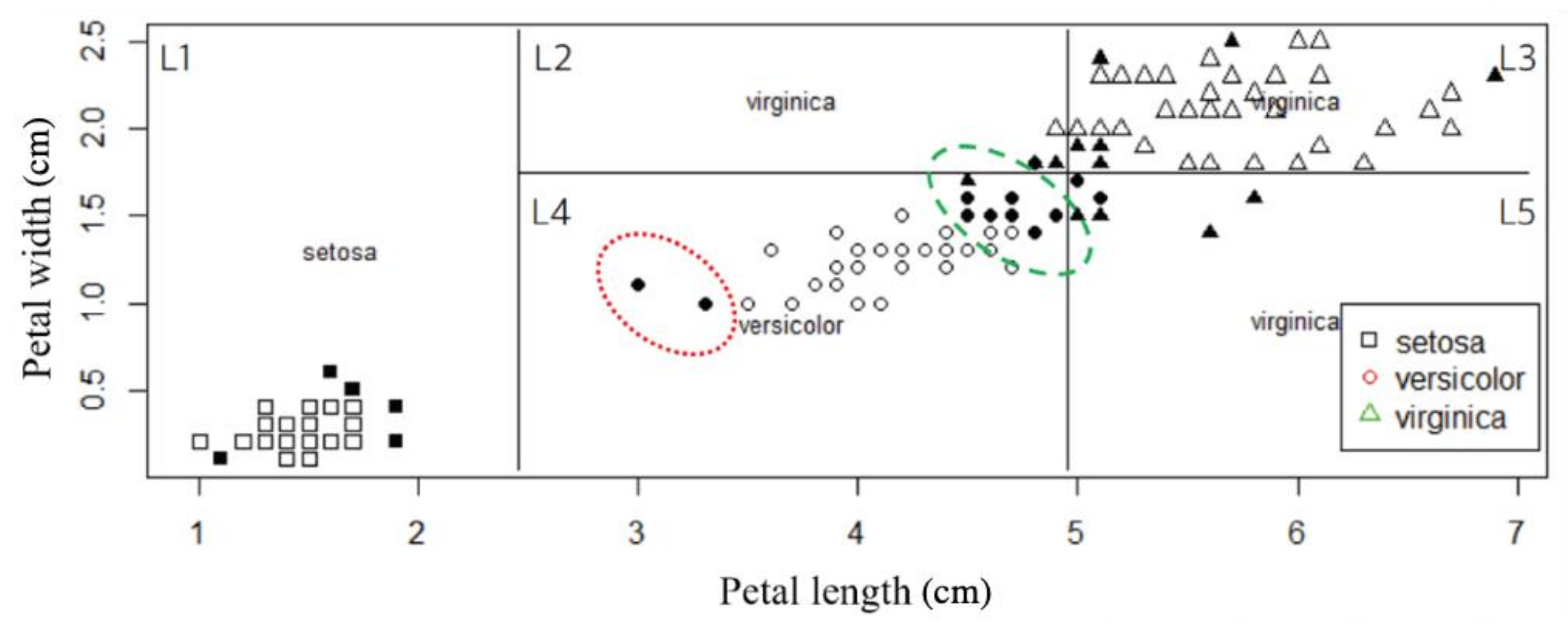
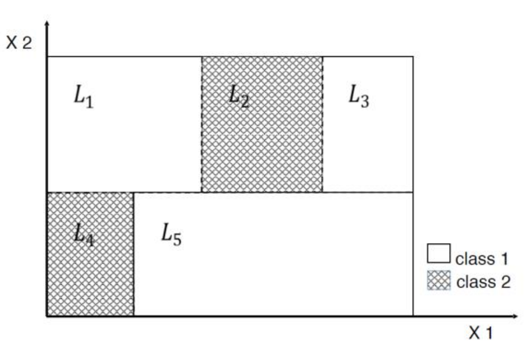
3.1. Distinct Adjacent Regions

After applying decision tree learning to the training data, we detect adjacent regions. The decision tree partitions the input space into several leaves (also denoted by terminal nodes) by reducing some impurity measures such as entropy. Following the approach of detecting adjacent regions introduced by Chau [25], we put in mathematical conditions for being adjacent regions and relate it to the relative support distance. Firstly, we represent each terminal node of a learned decision tree as follows:

$$L_q={\displaystyle \bigcap }_{j=1}^p{b}_{qj},l_{qj}\le b_{qj}\le h_{qj},$$

(5)

where $L_q$ is the $q$th leaf in the tree structure and $b_{qj}$ is the boundary range for the $j$th variable of the $q$th leaf with its lower bound $l_{qj}$ and upper bound $h_{qj}.$Recall that $p$ is the number of input variables. We should check whether each pair of leaves, $L_o$ and $L_q$, meet the following criteria:

$$h_{os}=l_{qs}or{l}_{os}=h_{qs},$$

(6)

$$l_{qk}\le l_{ok}\le h_{qk}or{l}_{qk}\le h_{ok}\le h_{qk},$$

(7)

where $s$ and $k$ are one of the input variables, $1\le s\le p$, $1\le k\le p$, and $s\ne k$. That is to say, if two leaves $L_o$ and $L_q$ are adjacent regions, they have to share one variable, represented by the variable $s$ in Equation (6), and one boundary, induced by the variable k in (7). Among all adjacent regions, we only consider distinct adjacent regions. For example, in Figure 2, the neighbors of $L_1$ are $L_2$, $L_4$, and $L_5$: $\left\{L_1,L_5\right\}$, however, does not form an adjacent region pair. {$L_3,L_5$} is an adjacent region pair but not distinct since those regions have the same majority class. Therefore, the distinct adjacent regions in the example are only $\left\{L_1,L_2\right\}$, $\left\{L_1,L_4\right\}$, $\left\{L_2,L_3\right\}$, $\left\{L_2,L_5\right\}$, and $\left\{L_4,L_5\right\}$. Distinct adjacent regions are summarized in Table 1. Now, we apply the measure of relative support distance to select support vector candidates in the found distinct adjacent regions for each region.

Figure 2. Distinct adjacent regions are $\left\{L_1,L_2\right\}$

, $\left\{L_1,L_4\right\}$, $\left\{L_2,L_3\right\}$, $\left\{L_2,L_5\right\}$, and $\left\{L_4,L_5\right\}$.

Table 1. Partition of input regions and distinct adjacent regions.

Region	Distinct Adjacent Regions
$L_1$	$L_2,L_4$
$L_2$	$L_1,L_3,L_5$
$L_3$	$L_2$
$L_4$	$L_1,L_5$
$L_5$	$L_2,L_4$

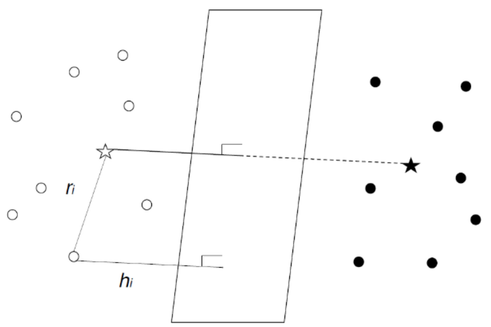
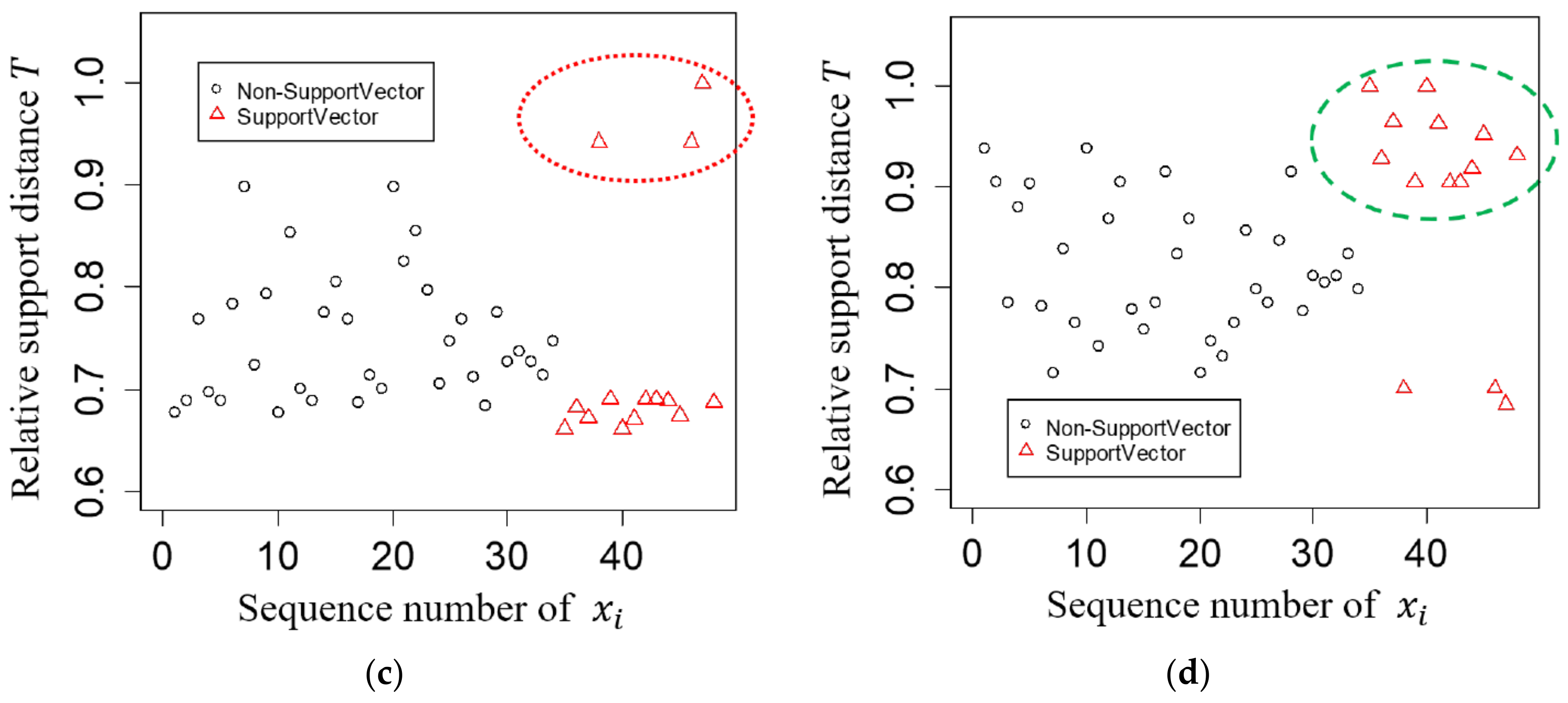
3.2. Relative Support Distance

Support vectors (SVs) play a substantial role in determining the decision hyperplane in contrast to non-SV data points. We extract data points in the training data that are most likely to be the support vectors, constructing a set of support vector candidates. Given two distinct adjacent regions $L_1$ and $L_2$ from the previous step, let us assume the majority class label of $L_1$ is $y=1$ and that of $L_2$, $y=2$ without loss of generality. First, we calculate the centroid (${\mathit{m}}_c$) for each majority class label as follows: for an index set $S_c=\left\{i\right|{\mathit{x}}_i\in L_c$ and the label of ${\mathit{x}}_i=c\}$,

$${\mathit{m}}_c=\frac{1}{n_c}{\displaystyle \sum }_{i\in S_c}{\mathit{x}}_i,$$

(8)

where $c\in \left\{1, 2\right\}$ and $n_c$ is the cardinality of index set $S_c$.

In other words, ${\mathit{m}}_c$ is the majority-class centroid of data points in $L_c$, of which the labels are $y=c$. Next, we create a virtual hyperplane that bisects the line from ${\mathit{m}}_1$ to ${\mathit{m}}_2$:

$$\begin{gathered} \mathit{M}=\frac{1}{2}\left({\mathit{m}}_1+{\mathit{m}}_2\right), \\ \mathit{W}={\mathit{m}}_1-{\mathit{m}}_2, \end{gathered}$$

(9)

where $M$ is the middle point of the two majority-class centroids. The virtual hyperplane is given by $H\left(\mathit{x}\right)=0$, where

$$H\left(\mathit{x}\right)={\mathit{W}}^t\left(\mathit{x}-\mathit{M}\right).$$

(10)

Lastly, we calculate the distance $r_x$ between each data point $x$ in $S_c$ and ${\mathit{m}}_c$ and the distance $h$ between each data point in $S_c$ and the virtual hyperplane $H\left(\mathit{x}\right)=0$:

$$\begin{gathered} r_{{\mathit{x}}_{c,l}}=\left|\left|{\mathit{x}}_{c,l}-{\mathit{m}}_c\right|\right|, \\ {h}_{{\mathit{x}}_{c,l}}=\frac{\left|H\left({\mathit{x}}_{c,l}\right)\right|}{\left|\left|\mathit{W}\right|\right|}=\frac{{\mathit{W}}^t\left({\mathit{x}}_{c,l}-\mathit{M}\right)}{\left|\left|{\mathit{m}}_1-{\mathit{m}}_2\right|\right|}, \end{gathered}$$

(11)

where ${\mathit{x}}_{c,l}$ is the $l$th data point belonging to $S_c$. Figure 3 shows a conceptual description of $r$ and $h$ using the virtual hyperplane in a leaf. After calculating $r_{\mathit{x}}$ and $h_{\mathit{x}}$, we apply feature scaling to bring all values into the range between 0 and 1. Our observation is that data points lying close to the virtual hyperplane are likely to be support vectors. In addition, data points lying close to the centroid are less likely to be support vectors. In light of these observations, we select data points lying near the hyperplane and far away from the centroid. For this purpose, we define the relative support distance $T\left(r_{\mathit{x}},h_{\mathit{x}}\right)$ as follows:

$$T\left(r_{\mathit{x}},h_{\mathit{x}}\right)=\frac{1}{\left(1+e^{-r_{\mathit{x}}}\right)h_{\mathit{x}}}.$$

(12)

Figure 3. Distances $r$ from the center and $h$ from the virtual hyperplane are shown. The two-star shapes are the centroid of each class.

The larger $T\left(r_{\mathit{x}},h_{\mathit{x}}\right)$ becomes, the more likely that the associated $\mathit{x}$ is a support vector.

The relationship between support vectors and distances $r$ and $h$ is illustrated in Figure 4. We use leaves $L_4$ with distinct adjacent regions $L_1$ and $L_2$ in Figure 1. In Figure 4, the observations marked by circles are non-support vectors while those by triangles (in red) are support vectors selected after training all data by SVMs. The distances $r$ and $h$ of $L_4$ relative to $L_1$ are in Figure 4a, and the relative support distance measures in Figure 4c. Likewise, those of L₄ relative to L₂ are in Figure 4b,d. We observe that the observations, marked by triangles and surrounded by a red ellipsoid in Figure 1, correspond to the support vectors surrounded by a red ellipsoid in region $L_4$ in Figure 4a, and they have larger values of relative support distance as shown in Figure 4c. Similarly, we notice that the observations, marked by triangles and surrounded by a green ellipsoid in Figure 4b, correspond to the support vectors surrounded by a green ellipsoid in region $L_4$ in Figure 1, and they also have larger values of relative support distance as shown in Figure 4d. The support vectors in $L_4$ are obtained by collecting observations with large values of relative support distance, for example by the rule $T\left(r_x,h_x\right)>0.9$, from both the pair of $L_4$ and $L_1$ and the pair of $L_4$ and $L_2$. The results reveal that the observations that have a mostly larger distance $r$ and shorter distance $h$ are likely to be support vectors.

Figure 4. Illustration of the distances $r$ and $h$ according to distinct adjacent regions for the iris data in Figure 1. (a) Distances for leaf $L_4$ relative to $L_1$ are shown. Notice the support vectors captured by leaf $L_4$ to leaf $L_1$ are in the (dotted) red ellipsoid. (b) Distances for leaf $L_4$ relative to $L_2$ are shown. Notice the support vectors captured by leaf $L_4$ relative to leaf $L_2$ are in the (dashed) green ellipsoid. (c) Relative support distances of the observations $x_i$ in leaf $L_4$ relative to $L_1$ are shown. Notice the support vectors captured by leaf $L_4$ to leaf $L_1$ are in the (dotted) red ellipsoid. (d) Relative support distances of the observations $x_i$ in leaf $L_4$ relative to $L_2$ are shown. Notice the support vectors captured by leaf $L_4$ relative to leaf $L_2$ are in the (dashed) green ellipsoid.

For each region, we calculate pairwise relative support distance with distinct adjacent regions and select a fraction of the observations, denoted by parameter $\beta$, in the decreasing order by $T\left(r_{\mathit{x}},h_{\mathit{x}}\right)$ as a candidate set of support vectors. That is to say, for each region, we select the top $\beta$ fraction of training data based on $T\left(r_{\mathit{x}},h_{\mathit{x}}\right)$. Parameter $\beta$ represents the proportion of the selected data points, between $0$ and $1$. For example, when $\beta$ is set to $1$, all data points are included in the training of SVMs. When $\beta =0.1$, we exclude $90\%$ of the data points and reduce the training data set to $10\%$. Finally, we combine relative support distance with random sampling, which means that a half of the training candidates are selected based on the proposed distance and the others are selected by random sampling. Though being quite informative for selecting possible support vectors, the proposed distance is calculated locally with distinct adjacent regions. Therefore, random sampling can compensate this property by providing whole data distribution information.

4. Experimental Results

In the experiments, we compare the proposed method, tree-based relative support distance (denoted by $\mathrm{TRSD}$), with some previously suggested methods, specifically SVMs with candidate vectors selection, denoted by $\mathrm{CVS}$ [18], and SVM with Fisher linear discriminant analysis, denoted by $\mathrm{FLD}$ [25], as well as standard SVMs, denoted by $\mathrm{SVM}$. For all comparing methods, we use LibSVM [15] since it is one of the fastest methods for training SVMs. The experiments are run on a computer with the following features: Core i5 3.4 GHz processor, 16.0 GB RAM, Windows 10 enterprise operating system. The algorithms are implemented in the R programming language. We use $18$ datasets which are from UCI Machine Learning Repository [35] and LibSVM Data Repository [36] except the checkerboard dataset [37]: a9a, banana, breast cancer, four-class, German credit, IJCNN-1 [38], iris, mushroom, phishing, Cod-RNA, skin segmentation, waveform, and w8a. Iris and Waveform datasets are modified for binary classification problems by assigning one class to positive and the others to negative. Table 2 shows a summary of the datasets used in the experiments where Size is the number of instances in dataset and Dim is the number of features.

Table 2. Datasets for experiments.

Dataset	Size	Dim	$\left|{\mathit{y}}_{\mathit{i}} = +1\right|$	$\left|{\mathit{y}}_{\mathit{i}} = -1\right|$
Iris-Setosa	150	4	50	100
Iris-Versicolor	150	4	50	100
Iris-Virginia	150	4	50	100
Breast Cancer	683	10	444	239
Four-class	862	2	555	307
Checkerboard	1000	2	514	486
German Credit	1000	24	700	300
Waveform-0	5000	21	1657	3343
Waveform-1	5000	21	1657	3343
Waveform-2	5000	21	1657	3343
Banana	5300	2	2924	2376
Mushroom	8124	112	3916	4208
Phishing	11,055	68	4898	6157
w8a	45,546	300	44,226	1320
a9a	48,842	123	37,155	11,687
IJCNN-1	141,691	22	128,126	13,565
Skin Segmentation	245,057	3	50,859	194,198
Cod-RNA	488,565	8	325,710	162,855

For testing, we apply three-fold cross validation, repeated three-times, by shuffling each dataset and dividing it into three parts, and use two parts as the training dataset, the other part as a testing dataset with different seeds. We use the RBF kernel for training SVMs in all tested methods. For each experiment, cross validation and grid search are used for tuning two hyper-parameters: the penalty factor $\mathrm{C}$ and the RBF kernel parameter $\mathsf{\gamma }$ in Equation (3). Hyper-parameters are searched by a two-dimensional grid with $\mathrm{C}\in \left\{0.1,1,10,100\right\}$ and $\mathsf{\gamma }\in \left\{0.001,0.01,0.1,1,1/p\right\}$ where $p$ is the number of features. Table 3 shows the values used for each dataset in the experiments. Moreover, we vary the fraction of data points in each region $\beta$ from $0.1$ to $0.3$ with the interval of $0.1$.

Table 3. Hyper-parameters setting for the experiments.

Method	Dataset	$\mathbf{Penalty}\mathbf{Factor}\mathit{C}$	$\mathbf{RBF}\mathbf{Kernel}\mathit{\gamma }$	Dataset	Penalty Factor C	RBF Kernel r
$\mathrm{SVM}$	Iris-Setosa	10	0.001	Waveform-2	0.1	$1/p$
$\mathrm{CVS}$		100	0.001		10	0.01
$\mathrm{FLD}$		100	0.001		100	0.001
$\mathrm{TRSD}$		100	0.001		1	$1/p$
$\mathrm{SVM}$	Iris-Versicolor	10	0.1	Banana	1	1
$\mathrm{CVS}$		100	0.1		100	1
$\mathrm{FLD}$		0.1	0.01		10	$1/p$
$\mathrm{TRSD}$		10	1		1	1
$\mathrm{SVM}$	Iris-Virginia	100	0.01	Mushroom	100	0.001
$\mathrm{CVS}$		100	0.01		10	0.001
$\mathrm{FLD}$		100	0.001		0.1	0.01
$\mathrm{TRSD}$		100	0.1		100	0.001
$\mathrm{SVM}$	Breast Cancer	1	0.01	Phishing	10	$1/p$
$\mathrm{CVS}$		10	0.001		1	0.01
$\mathrm{FLD}$		100	0.001		100	0.001
$\mathrm{TRSD}$		1	0.1		100	0.001
$\mathrm{SVM}$	Four-class	10	1	w8a	10	0.001
$\mathrm{CVS}$		100	1		10	0.01
$\mathrm{FLD}$		100	1		1	0.001
$\mathrm{TRSD}$		10	1		10	0.001
$\mathrm{SVM}$	Checkerboard	100	1	a9a	10	0.001
$\mathrm{CVS}$		100	1		10	0.01
$\mathrm{FLD}$		100	1		100	0.001
$\mathrm{TRSD}$		100	1		10	0.001
$\mathrm{SVM}$	German Credit	100	0.001	IJCNN-1	10	0.1
$\mathrm{CVS}$		1	$1/p$		100	$1/p$
$\mathrm{FLD}$		0.1	0.001		100	0.01
$\mathrm{TRSD}$		1	0.01		10	$1/p$
$\mathrm{SVM}$	Waveform-0	1	0.01	Skin Segmentation	100	1
$\mathrm{CVS}$		10	0.01		100	1
$\mathrm{FLD}$		1	0.01		100	0.1
$\mathrm{TRSD}$		1	0.01		100	1
$\mathrm{SVM}$	Waveform-1	1	$1/p$	Cod-RNA	10	1
$\mathrm{CVS}$		10	$1/p$		100	0.001
$\mathrm{FLD}$		1	$1/p$		100	0.01
$\mathrm{TRSD}$		1	$1/p$		10	$1/p$

We compare the performance of $\mathrm{SVM}$, $\mathrm{CVS}$, $\mathrm{FLD}$, and $\mathrm{TRSD}$ in terms of classification accuracy and the training time (in seconds), summarized in Table 4. We also depicted the performance comparison of the proposed $\mathrm{TRSD}$ with $\mathrm{CVS}$ and $\mathrm{FLD}$ on the five largest datasets when $\beta =0.1$ in Figure 5. We used log-2 scale for y-axis in Figure 5b. In Table 4, Acc is the accuracy on test data; $\sigma$ is the standard deviation; and Time is the training time in seconds. Even though the accuracy of the proposed algorithm is slightly degraded in a few cases, it is higher than that of $\mathrm{CVS}$ and $\mathrm{FLD}$ in most cases. In addition, as $\beta$ is greater, the accuracy of the proposed algorithm enhanced substantially. For small datasets, there is no significant improvement on computation time compared to the standard SVM since those datasets are already small enough. However, we notice that the training time of $\mathrm{TRSD}$ improved quite much when using the large-scale datasets.

Table 4. Comparisons in terms of accuracy and time on datasets (the results of support vector machines (SVM) are not bolded, because it had access to all examples).

Dataset	$\mathbf{S}\mathbf{V}\mathbf{M}$			$\mathbf{C}\mathbf{V}\mathbf{S}$			$\mathbf{F}\mathbf{L}\mathbf{D}$			$\mathbf{T}\mathbf{R}\mathbf{S}\mathbf{D}$
	acc	$\mathit{\sigma }$	Time	acc	$\mathit{\sigma }$	Time	Acc	$\mathit{\sigma }$	Time	Acc	$\mathit{\sigma }$	Time
$\beta =0.1$
Iris-Setosa	100	0	0.01	100	0	0.01	100	0	0.01	100	0	0.01
Iris-Versicolor	95.43	0.98	0.01	78.54	12.71	0.01	52.29	17.53	0.02	87.71	2.22	0.02
Iris-Virginia	96.57	2.24	0.01	87.99	6.55	0.01	91.71	4.07	0.02	91.5	4.72	0.01
Breast Cancer	96.99	0.89	0.01	95.36	0.5	0.01	96.3	0.95	0.08	96.24	1.04	0.04
Four-class	100	0	0.01	93.19	0.08	0.01	93.28	3.58	0.07	93.24	2.4	0.05
Checkerboard	94.3	0.63	0.03	84.61	1.47	0.01	-	-	-	79.34	3.13	0.08
German Credit	75.7	0.7	0.09	69.87	0.75	0.01	70	0.04	0.42	70.55	0.97	0.21
Waveform-0	89.85	0.63	1.03	85.5	0.73	0.21	87.51	0.65	0.58	89.01	0.51	0.34
Waveform-1	91.26	0.3	0.68	83.7	0.87	0.2	89.46	0.38	0.66	90.06	0.5	0.35
Waveform-2	91.76	0.48	0.94	84.52	1.23	0.21	89.77	0.97	0.74	90.31	0.48	0.38
Banana	90.6	0.69	0.59	64.13	2.69	0.03	83.46	1.77	0.09	88.8	0.4	0.06
Mushroom	100	0	1.47	90.67	0.62	2.08	84.99	7.23	1.11	99.83	0.12	0.79
Phishing	96.69	0.26	4.59	90	0.49	2.28	93.28	0.69	1.46	93.96	0.26	0.79
w8a	99.11	0.04	114.85	97.4	0.05	19.64	97.83	0.3	231.89	98.38	0.09	51.18
a9a	84.7	0.14	373.24	78.48	0.29	43.19	81.27	0.72	21.91	84.24	0.16	12.59
IJCNN-1	99.27	0.7	224.29	97.02	0.12	9.83	97.55	0.1	12	98.39	0.05	7.71
Skin Segmentation	99.94	0	20.23	99.93	0.01	1.27	99.45	0.11	3.39	99.89	0.01	2.51
Cod-RNA	96.98	0.03	4425.55	90.68	0.08	178.3	96.05	0.08	66.93	96.32	0.03	42.85
$\beta =0.2$
Iris-Setosa	100	0	0.01	100	0	0.01	100	0	0.01	100	0	0.01
Iris-Versicolor	95.43	0.98	0.01	89.44	3.92	0.01	51.72	17.02	0.02	93.43	1.48	0.02
Iris-Virginia	96.57	2.24	0.01	93.43	2.2	0.01	94.26	2.17	0.02	90.31	3.03	0.02
Breast Cancer	96.99	0.89	0.01	95.55	1.09	0.01	96.49	0.91	0.07	96.3	0.95	0.06
Four-class	100	0	0.01	96.42	1.78	0.01	95.38	1.63	0.07	98.81	0.8	0.05
Checkerboard	94.3	0.63	0.03	93.66	1.09	0.01	-	-	-	83.66	2.48	0.08
German Credit	75.7	0.7	0.09	70.04	0.01	0.02	70	0.04	0.35	70.56	0.62	0.25
Waveform-0	89.85	0.63	1.03	88.35	0.37	0.27	88.55	0.73	0.76	89.28	0.73	0.54
Waveform-1	91.26	0.3	0.68	86.45	0.56	0.26	89.89	0.37	0.78	90.52	0.49	0.5
Waveform-2	91.76	0.48	0.94	88.21	0.5	0.27	90.39	0.54	0.99	90.62	0.58	0.51
Banana	90.6	0.69	0.59	79.86	2.02	0.1	85.14	1.5	0.1	89.69	0.36	0.07
Mushroom	100	0	1.47	97.09	1.12	2.22	97.37	0.88	1.33	99.91	0.1	0.85
Phishing	96.69	0.26	4.59	93.91	0.2	2.58	94.42	0.38	1.63	94.62	0.3	0.99
w8a	99.11	0.04	114.85	97.5	0.07	27.22	98.12	0.12	233.78	98.63	0.05	63.04
a9a	84.7	0.14	373.24	78.86	0.26	74.22	82.19	0.42	39.37	84.61	0.18	24.27
IJCNN-1	99.27	0.7	224.29	98.41	0.05	23.56	98.07	0.09	18.7	98.72	0.07	14.45
Skin Segmentation	99.94	0	20.23	99.94	0.01	2.36	99.73	0.06	4.82	99.9	0.01	3.64
Cod-RNA	96.98	0.03	4425.55	95.44	0.03	514.9	96.19	0.03	293.29	96.43	0.03	152.98
$\beta =0.3$
Iris-Setosa	100	0	0.01	100	0	0.01	100	0	0.01	100	0	0.01
Iris-Versicolor	95.43	0.98	0.01	92.3	2.44	0.01	59.87	14.47	0.01	94.01	2.57	0.02
Iris-Virginia	96.57	2.24	0.01	93.98	2.03	0.01	95.51	2.53	0.01	94.31	1.77	0.02
Breast Cancer	96.99	0.89	0.01	96.42	0.69	0.01	96.36	0.55	0.08	96.17	0.79	0.05
Four-class	100	0	0.01	96.62	1.52	0.01	95.62	1.6	0.07	99.5	0.66	0.05
Checkerboard	94.3	0.63	0.03	93.96	1	0.01	-	-	-	87.18	2.3	0.1
German Credit	75.7	0.7	0.09	69.95	0.22	0.03	70	0.04	0.35	70.81	0.87	0.29
Waveform-0	89.85	0.63	1.03	89.1	0.38	0.35	88.93	0.71	0.71	89.47	0.34	0.41
Waveform-1	91.26	0.3	0.68	87.49	0.33	0.34	90.18	0.46	0.74	90.8	0.34	0.38
Waveform-2	91.76	0.48	0.94	89.63	0.43	0.33	90.71	0.66	0.84	91.09	0.63	0.41
Banana	90.6	0.69	0.59	81.47	0.74	0.17	86.63	1.83	0.12	90.09	0.49	0.1
Mushroom	100	0	1.47	97.79	0.71	2.17	97.87	0.28	1.71	99.95	0.07	0.97
Phishing	96.69	0.26	4.59	94.51	0.16	3	94.75	0.3	1.99	94.93	0.14	1.29
w8a	99.11	0.04	114.85	97.71	0.08	49.63	98.36	0.07	237.01	98.83	0.06	55.09
a9a	84.7	0.14	373.24	80.35	0.2	127.4	83.18	0.28	77.18	84.68	0.13	43.02
IJCNN-1	99.27	0.7	224.29	98.68	0.06	37.79	98.3	0.08	34.75	98.86	0.06	25.43
Skin Segmentation	99.94	0	20.23	99.94	0.01	3.84	99.75	0.08	7.01	99.91	0	3.78
Cod-RNA	96.98	0.03	4425.55	95.92	0.04	899.1	96.27	0.01	598.23	96.48	0.02	256.71

Figure 5. Comparison of the proposed tree-based relative support distance (TRSD) with candidate vectors (CVS) and Fisher linear discriminant analysis (FLD) on the five largest datasets.

For statistical analysis, we also performed Friedman test to see that there exists significant difference between the multiple comparing methods in terms of accuracy. If the null hypothesis of the Friedman test is rejected, we performed Dunn’s test. Table 5 shows the summary of the Dunn’s test results at the significant level $\alpha =0.05$. In Table 5, the entries (1) $\mathrm{TRSD}>\mathrm{CVS}\left(\mathrm{FLD}\right)$; (2) $\mathrm{TRSD}\approx \mathrm{CVS}\left(\mathrm{FLD}\right)$; (3) $\mathrm{TRSD}<\mathrm{CVS}\left(\mathrm{FLD}\right)$, respectively, denote that: (1) the performance of $\mathrm{TRSD}$ is significantly better than $\mathrm{CVS}\left(\mathrm{FLD}\right)$; (2) there in no significant difference between the performances of $\mathrm{TRSD}$ and $\mathrm{CVS}\left(\mathrm{FLD}\right)$; and (3) the performance of $\mathrm{TRSD}$ is significantly worse than $\mathrm{CVS}\left(\mathrm{FLD}\right)$. Each number in Table 5 means the number of datasets. At $\beta =0.1$, our proposed method is significantly better than $\mathrm{CVS}$ and $\mathrm{FLD}$ in 10 and 9 cases among 18 datasets. These numbers increase to 11 and 10 at $\beta =0.3$. On the other hand, our proposed method is significantly worse than $\mathrm{CVS}$ only in 2, 3 and 3 cases; than $\mathrm{FLD}$ in 0, 1 and 0 cases at $\beta =0.1,0.2,0.3$ respectively. Based on the observations in the experiments, we can conclude that our proposed method generates an effective reduction of the training datasets while producing better performance than the existing data reduction approaches.

Table 5. Dunn’s test results in different $\beta$ for the significant level $\alpha =0.05$.

$\mathit{\beta }$	$\mathbf{T}\mathbf{R}\mathbf{S}\mathbf{D} > \mathbf{C}\mathbf{V}\mathbf{S}$	$\mathbf{T}\mathbf{R}\mathbf{S}\mathbf{D} \approx \mathbf{C}\mathbf{V}\mathbf{S}$	$\mathbf{T}\mathbf{R}\mathbf{S}\mathbf{D} < \mathbf{C}\mathbf{V}\mathbf{S}$	$\mathbf{T}\mathbf{R}\mathbf{S}\mathbf{D} > \mathbf{F}\mathbf{L}\mathbf{D}$	$\mathbf{T}\mathbf{R}\mathbf{S}\mathbf{D} \approx \mathbf{F}\mathbf{L}\mathbf{D}$	$\mathbf{T}\mathbf{R}\mathbf{S}\mathbf{D} < \mathbf{F}\mathbf{L}\mathbf{D}$
0.1	10	6	2	9	9	0
0.2	11	4	3	9	8	1
0.3	11	4	3	10	8	0
Total	32	14	8	28	25	1

Finally, to compare the training time of $\mathrm{SVM}$, $\mathrm{CVS}$, $\mathrm{FLD}$, and $\mathrm{TRSD}$ in detail, we divide it into two parts: selecting candidate vectors ($\mathrm{SC}$) and training a final SVM model ($\mathrm{TS}$) when $\beta =0.3$, summarized in Table 6. From Table 6, we can notice that it especially takes longer time for $\mathrm{TRSD}$ and $\mathrm{FLD}$ than $\mathrm{CVS}$ to select candidate vectors with w8a dataset. This is because the time complexity of building a decision tree is $O\left(pn \log n\right)$ where $p$ is the number of features and $n$ is the size of training dataset. However, our proposed method takes shorter than $\mathrm{FLD}$ since calculating $\mathrm{TRSD}$ is more computationally efficient than fisher linear discriminant and is the fastest overall. The results in Table 6 show that the proposed method efficiently selects support vector candidates while maintaining good classification performance.

Table 6. Time comparison in detail. $\mathrm{SC}$ and $\mathrm{TS}$ mean computing time for selecting candidate vectors and training a final SVM model respectively.

Dataset	SVM		CVS		FLD		TRSD
	SC	TS	SC	TS	SC	TS	SC	TS
Iris-Setosa	0	0.01	0	0.01	0	0.01	0	0.01
Iris-Versicolor	0	0.01	0	0.01	0	0.01	0	0.01
Iris-Virginia	0	0.01	0	0.01	0	0.01	0	0.01
Breast Cancer	0	0.01	0	0.01	0.07	0.01	0.04	0.01
Four-class	0	0.01	0	0.01	0.06	0.01	0.04	0.01
Checkerboard	0	0.03	0	0.01	-	-	0.09	0.01
German Credit	0	0.09	0.01	0.02	0.33	0.02	0.27	0.02
Waveform-0	0	1.03	0.18	0.17	0.58	0.13	0.3	0.11
Waveform-1	0	0.68	0.17	0.17	0.65	0.09	0.3	0.08
Waveform-2	0	0.94	0.17	0.16	0.73	0.11	0.34	0.07
Banana	0	0.59	0	0.17	0.08	0.04	0.05	0.05
Mushroom	0	1.47	1.9	0.27	0.99	0.72	0.71	0.26
Phishing	0	4.59	2.08	0.92	1.3	0.69	0.72	0.57
w8a	0	114.85	17.48	32.15	228.83	8.18	46.35	8.74
a9a	0	373.24	44.5	82.88	16.52	60.66	8.84	34.18
IJCNN-1	0	224.29	6.06	31.73	10.08	24.67	5.77	19.66
Skin Segmentation	0	20.23	0.3	3.54	3.22	3.79	2.3	1.48
Cod-RNA	0	4425.55	0.7	898.4	15.46	582.77	11.24	245.47

5. Discussion and Conclusions

In this study, we have proposed a tree-based data reduction approach for solving large-scale SVM problems. In order to reduce time consumption in training SVM models, we apply a novel support vector selection method combining tree decomposition and the proposed relative support distance. We introduce the relative distance measure along with a virtual hyperplane between two distinct adjacent regions to effectively exclude non-SV data points. The virtual hyperplane, easily obtainable, takes advantage of the decomposed tree structures and is shown to be effective in selecting support vector candidates. In computing the relative support distance, we also use the distance between each data point to the centroid in each region and combine the two in consideration of the nonlinear characteristics of support vectors. In experiments, we have demonstrated that the proposed method outperforms some existing methods for selecting support vector candidates in terms of computation time and classification performance. In the future, we would like to investigate other large-scale SVM problems such as multi-class classification and support vector regression. We also envision an extension of the proposed method to under-sampling techniques.

References

- Cortes, C.; Vapnik, V. Support-Vector Networks. Mach. Learn. 1995, 20, 273–297. [Google Scholar] [CrossRef]
- Cristianini, N.; Shawe-Taylor, J. An Introduction to Support Vector Machines and other Kernel-Based Learning Methods; Cambridge University Press: Cambridge, UK, 2000. [Google Scholar]
- Cai, Y.D.; Liu, X.J.; biao Xu, X.; Zhou, G.P. Support Vector Machines for predicting protein structural class. BMC Bioinform. 2001, 2, 3. [Google Scholar] [CrossRef] [PubMed]
- Belongie, S.; Malik, J.; Puzicha, J. Shape Matching and Object Recognition Using Shape Contexts. IEEE Trans. Pattern Anal. Mach. Intell. 2002, 24, 509–522. [Google Scholar] [CrossRef]
- Ahn, H.; Lee, K.; Kim, K.j. Global Optimization of Support Vector Machines Using Genetic Algorithms for Bankruptcy Prediction. In Proceedings of the 13th International Conference on Neural Information Processing—Volume Part III; Springer: Berlin, Germany, 2006; pp. 420–429. [Google Scholar]
- Bayro-Corrochano, E.J.; Arana-Daniel, N. Clifford Support Vector Machines for Classification, Regression, and Recurrence. IEEE Trans. Neural Netw. 2010, 21, 1731–1746. [Google Scholar] [CrossRef] [PubMed]
- Boser, B.E.; Guyon, I.M.; Vapnik, V.N. A Training Algorithm for Optimal Margin Classifiers. Proceedings of the Fifth Annual Workshop on Computational Learning Theory; Association for Computing Machinery: New York, NY, USA, 1992; pp. 144–152. [Google Scholar]
- Friedman, J.; Hastie, T.; Tibshirani, R. The Elements of Statistical Learning; Springer: Berlin, Germany, 2001; Volume 1. [Google Scholar]
- Qiu, J.; Wu, Q.; Ding, G.; Xu, Y.; Feng, S. A survey of machine learning for big data processing. EURASIP J. Adv. Signal. Process. 2016, 2016, 1–16. [Google Scholar]
- Liu, P.; Choo, K.K.R.; Wang, L.; Huang, F. SVM of Deep Learning? A Comparative Study on Remote Sensing Image Classification. Soft Comput. 2017, 21, 7053–7065. [Google Scholar] [CrossRef]
- Chapelle, O. Training a support vector machine in the primal. Neural Comput. 2007, 19, 1155–1178. [Google Scholar] [CrossRef] [PubMed]
- Platt, J.C. 12 fast training of support vector machines using sequential minimal optimization. Adv. Kernel Methods 1999, 185–208. [Google Scholar]
- Joachims, T. Svmlight: Support Vector Machine. SVM-Light Support. Vector Mach. Univ. Dortm. 1999, 19.. Available online: http://svmlight.joachims.org (accessed on 29 November 2019).
- Vishwanathan, S.; Murty, M.N. SSVM: A simple SVM algorithm. 2002 International Joint Conference on Neural Networks. IJCNN’02, Honolulu, HI, USA, 12–17 May 2002. [Google Scholar]
- Chang, C.C.; Lin, C.J. LIBSVM: A library for support vector machines. ACM Trans. Intell. Syst. Technol. (TIST) 2011, 2, 27. [Google Scholar] [CrossRef]
- Lee, Y.J.; Mangasarian, O.L. RSVM: Reduced Support Vector Machines. SDM. In Proceedings of the 2001 SIAM International Conference on Data Mining, Chicago, IL, USA, 5–7 April 2001; pp. 325–361. [Google Scholar]
- Collobert, R.; Bengio, S.; Bengio, Y. A parallel mixture of SVMs for very large scale problems. Neural Comput. 2002, 14, 1105–1114. [Google Scholar] [CrossRef] [PubMed]
- Li, M.; Chen, F.; Kou, J. Candidate vectors selection for training support vector machines. In Natural Computation, 2007. ICNC 2007. In Proceedings of the Third International Conference on Natural Computation, Haikou, China, 24–27 August 2007; pp. 538–542. [Google Scholar]
- Nishida, K.; Kurita, T. RANSAC-SVM for large-scale datasets. In Proceedings of the 19th International Conference on Pattern Recognition, Tampa, FL, USA, 8–11 December 2008; pp. 1–4. [Google Scholar]
- Kawulok, M.; Nalepa, J. Support Vector Machines Training Data Selection Using a Genetic Algorithm. In Proceedings of the 2012 Joint IAPR International Conference on Structural, Syntactic, and Statistical Pattern Recognition; Springer: Berlin, Germany, 2012; pp. 557–565. [Google Scholar]
- Nalepa, J.; Kawulok, M. A Memetic Algorithm to Select Training Data for Support Vector Machines. In Proceedings of the 2014 Annual Conference on Genetic and Evolutionary Computation, Association for Computing Machinery, New York, NY, USA, 12–16 July 2014; pp. 573–580. [Google Scholar]
- Nalepa, J.; Kawulok, M. Adaptive Memetic Algorithm Enhanced with Data Geometry Analysis to Select Training Data for SVMs. Neurocomputing 2016, 185, 113–132. [Google Scholar] [CrossRef]
- Martin, J.K.; Hirschberg, D. On the complexity of learning decision trees. International Symposium on Artificial Intelligence and Mathematics. Citeseer 1996, 112–115. [Google Scholar]
- Chang, F.; Guo, C.Y.; Lin, X.R.; Lu, C.J. Tree decomposition for large-scale SVM problems. J. Mach. Learn. Res. 2010, 11, 2935–2972. [Google Scholar]
- Chau, A.L.; Li, X.; Yu, W. Support vector machine classification for large datasets using decision tree and fisher linear discriminant. Future Gener. Comput. Syst. 2014, 36, 57–65. [Google Scholar] [CrossRef]
- Cervantes, J.; Garcia, F.; Chau, A.L.; Rodriguez-Mazahua, L.; Castilla, J.S.R. Data selection based on decision tree for SVM classification on large data sets. Appl. Soft Comput. 2015, 37, 787–798. [Google Scholar] [CrossRef]
- Radial Basis Function Kernel, Wikipedia, Wikipedia Foundation. Available online: https://en.wikipedia.org/wiki/Radial_basis_function_kernel (accessed on 29 November 2019).
- Kass, G.V. An Exploratory Technique for Investigating Large Quantities of Categorical Data. J. R. Stat. Soc. 1980, 29, 119–127. [Google Scholar] [CrossRef]
- Breiman, L.; Friedman, J.H.; Olshen, R.A.; Stone, C.J. Classification and Regression Trees; Wadsworth and Brooks: Monterey, CA, USA, 1984. [Google Scholar]
- Quinlan, J.R. C4.5: Programs for Machine Learning; Morgan Kaufmann Publishers Inc.: San Francisco, CA, USA, 1993. [Google Scholar]
- Loh, W.Y.; Shih, Y.S. Split Selection Methods for Classification Trees. Stat. Sin. 1997, 7, 815–840. [Google Scholar]
- Martin, J.K.; Hirschberg, D.S. The Time Complexity of Decision Tree Induction; University of California: Irvine, CA, USA, 1995. [Google Scholar]
- Li, X.B.; Sweigart, J.; Teng, J.; Donohue, J.; Thombs, L. A dynamic programming based pruning method for decision trees. Inf. J. Comput. 2001, 13, 332–344. [Google Scholar] [CrossRef]
- Fisher, R.A. The use of multiple measurements in taxonomic problems. Ann. Eugen. 1936, 7, 179–188. [Google Scholar] [CrossRef]
- Dua, D.; Graff, C. UCI Machine Learning Repository; University of California, School of Information and Computer Science: Irvine, CA, USA, 2019. [Google Scholar]
- Chang, C.C.; Lin, C.J. LIBSVM: A Library for Support Vector Machines. ACM Transactions on Intelligent Systems and Technology, 2:27:1—27:27. 2011. Available online: https://www.csie.ntu.edu.tw/cjlin/libsvmtools/datasets/binary.html (accessed on 29 November 2019).
- Ho, T.K.; Kleinberg, E.M. Checkerboard Data Set. 1996. Available online: https://research.cs.wisc.edu/math-prog/mpml.html (accessed on 29 November 2019).
- Prokhorov, D. IJCNN 2001 Neural Network Competition.Slide Presentation in IJCNN’01, Ford Research Laboratory. 2001. Available online: https://www.csie.ntu.edu.tw/~cjlin/libsvmtools/datasets/binary.html (accessed on 29 November 2019).