1. Introduction
ECG signals can be easily acquired by putting one’s finger on the sensor for about 30 s [
1]. There are at least two types of important information contained in the ECG signal, including those related to health or biomedical [
2,
3,
4] and those related to the person identification or biometrics [
5,
6,
7]. Due to its convenience, many ECG classification algorithms have been developed, including handcraft [
4,
8,
9] and machine learning [
10,
11,
12,
13,
14,
15] methods. The handcraft method is rather difficult to utilize on non-stationary signals, such as ECG, while machine learning methods normally require high computational resources. Due to its high accuracy, the machine learning method is preferable compared to the handcraft method. However, an efficient algorithm is required to minimize the computational requirements while still maintaining its high accuracy.
Many researches have been conducted on the implementation of handcraft techniques, including the extraction of time-based ECG features using Fourier [
8] and wavelet [
4,
9] transforms. Both Fourier and wavelet transform can be used for ECG beats detection (QRS detection), as well as feature extraction, such as R-peak, RR-interval, T-wave region, and QT-zone. After QRS detection, amplitude and duration-based ECG features can also be measured using weighted diagnostic distortion (WDD) [
16]. The feature extraction stage is usually followed by a classification stage with various methods such as vector quantization [
17], random forest [
18,
19,
20], k-nearest neighbor (kNN) [
10,
20,
21], support vector machine (SVM) [
10,
13,
18,
20], multi-layer perceptron (MLP) [
22,
23,
24] and convolutional neural network (CNN) [
25].
If the feature extraction and classification stages are done separately, SVM can be used and optimized using particle swarm optimization (PSO) [
10]. As presented in [
10], after supervised training was conducted using 500 beats, the model can classify 40,438 test beats into five classes with accuracy of 89.72%, outperforming the other methods such as kNN or radial basis function (RBF). Nevertheless, the quality of this classification can still be improved in terms of increasing the number of classes and/or accuracy. For example, discrete orthogonal Stockwell transform (DOST) could be used during feature extraction followed by principal component analysis (PCA) to reduce feature dimensions [
13]. As shown in [
13], after supervised training was conducted on 23,996 beats, the remainder 86,113 test beats could be classified into 16 classes with better accuracy of 98.82%.
Another promising method for improving efficiency is by combining both feature extraction and classification stages using MLP [
26] and CNN [
27]. For example, in [
27], a neural network model containing three layers of CNN and two layers of MLP was proposed. The input of this model is a raw ECG beat signal containing 64 or 128 samples centered on the R-peak. While the number of ECG beats used for training is kept at minimum at 245 and the testing beats is set to 100,144, it can achieve accuracy of 95.14% to classify five classes. In [
28], autoencoder was utilized with a rather good result but it needs to fairly evaluate the performance with and without denoising. Moreover, the deep networks configuration could be further optimized to reduce computational time.
Although many researches have been conducted, an efficient algorithm for cardiac arrhythmia classification is still required. Therefore, the objective of this paper was to simplify the overall process to lower the computational cost, while maintaining high accuracy. A neural network model presented in [
27] was adopted and modified to now classify 16 classes as in [
13]. The performance of our proposed algorithms was evaluated using number of classes, prediction stages, and accuracy.
2. 1D Convolutional Neural Network and Its Enhancement
In this paper, we use two stages of ECG classification, namely beat segmentation and classification. For classification purposes, CNN could be used as stated in [
27,
29]. Although CNN hyperparameters such as number of filters, filter size, padding type, activation type, pooling, backpropagation, still have to be done intuitively or by trial and error, there are still some techniques that can be used to reduce the amount of trial and error attempts to achieve the best results. Further enhancement to the CNN could be done using All Convolutional Network (ACN) [
30], Batch Normalization (BN) [
31]. Depthwise Separable Convolution (DSC) [
32], ensemble CNN [
33], which are further elaborated in this section. Out of various methods for CNN enhancement, DSC has the greatest effect on decreasing training time, while ensemble CNN enables further improvement on the classification rate.
ACN is used to replace pooling layer with stride during convolution. Pooling or stride is used for downsampling as CNN output parameters are less than the input parameter. In our case, the CNN input parameter is set to 256, while the output parameter is set to 16. Normally, the last or output layer of CNN uses the SoftMax activation function to determine the output class based on its highest probability. To reduce the number of layers, pooling layer could be replaced with stride during convolution [
30].
Input normalization is required to solve internal covariate shift, i.e., the change in the distribution of network activations due to the change in network parameters during training. Without normalization, this will slow down the training iteration or even stop the iteration before reaching adequate accuracy. To solve this issue, BN can be conducted for each training mini-batch [
31]. To reduce computational cost, BN could be conducted during the convolution process before nonlinear activation, such as rectified linear unit (ReLU). On the other hand, DSC could be used to reduce the number of parameters and floating points multiplication operation, with negligible performance degradation [
34]. DSC could be performed on one layer or a group of layers of CNNs.
Another thing that must be considered in designing the CNN model is the implementation of the Flatten layer before the Fully Connected (FC) layer. Even though Flatten technically can be replaced by the AveragePool layer, these two techniques differ in terms of execution time and the final results obtained. The Flatten process does not require any further calculations, it only changes the arrangement of parameters in the last layer, while AveragePool must perform arithmetic operations to get the average value of each group in the last layer according to its position. The next effect of Flatten causes more neurons connected to FC, in comparison to the number of neurons produced by AveragePool which is obviously related to the number of arithmetic operations at the FC layer. It should be noted that the number of neurons in the Flatten layer represents all local features on the last layer without having to be combined in the average value.
2.1. 1-D CNNs
As described in [
27,
29], during the forward propagation, the input map of the next layer neuron will be obtained by the cumulation of the final output maps of the previous layer neurons convolved with their individual kernels as follows:
where
is 1-D convolution,
is the input,
is the bias of the
-th neuron at layer
,
is the output of the
-th neuron at layer
,
is the kernel (weight) from the
-th neuron at layer
to the
-th neuron at layer
. Let
and
be the input and output layers, respectively. The inter backpropagation delta error of the output
can be expressed as follows:
where
flips the array, and
performs full convolution in 1-D with
zero padding. Lastly, the weight and bias sensitivities can be expressed as follows:
2.2. All Convolutional Network
All Convolutional Network (ACN) [
30] is utilized by removing the max pooling layer and replacing it with convolutional stride. As a result, the computational cost will be reduced, as it removes several layers as well as reducing the floating point operation on the convolution operation. For example, conv stride = 1 continued with max pooling 2 could be replaced with one layer, i.e., conv stride = 2 with an almost similar result.
Let
denote a feature map produced by some layer of a CNN, while
is the number of filters in this layer. Then
-norm subsampling with pooling size
(or half-length
) and stride
applied to the feature map
is a 3-dimensional array
with the following entries:
where
is the function mapping from positions in
to positions in
representing the stride,
is the order of the p-norm (
represents max pooling). If
, pooling regions do not overlap. The standard definition of a convolution layer
applied to the feature map
is given as:
where
are the convolutional weights,
is the activation function, typically a rectified linear activation ReLU
, and
is the number of output features of the convolutional layer. From the two equations, it is evident that the computational cost will be reduced.
2.3. Batch Normalization
Batch Normalization (BN) is intended to avoid non-linear saturation or internal covariate shifts causing a faster learning process [
31]. The Batch Normalization allows much higher learning rates and reduces dependence on the initialization process. It can also act as a regularizer to reduce the generalization error and to avoid overfitting without the implementation of dropout layer. To reduce computation, the Batch Normalization is carried out directly after the convolution and before ReLU. ReLU before BN can mess up the calculations due to the non-linear nature of ReLU. Suppose we have network activation as follows:
where
and
are learned parameters of the model, and
is the nonlinear activation function such as sigmoid or ReLU. Since we normalize
, the bias
can be ignored since its effect will be cancelled by the subsequent mean subtraction. Therefore, Equation (7) is replaced with:
where the
transform is applied indenpendently to each dimension of
, with a separate pair of learned parameters.
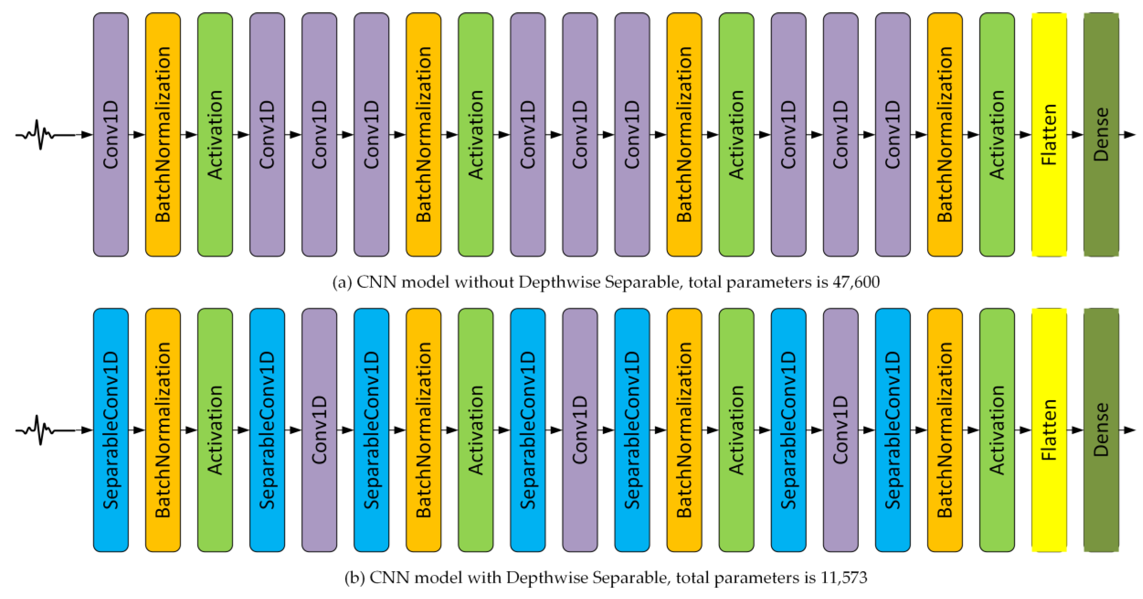
2.4. Depthwise Separable Convolution
In addition to the implementation of BN, the convolution part can also be further optimized, for example by using depthwise separable convolution (DSC) to reduce the computational costs by reducing the number of arithmetic operations while preserving the same final results [
32,
34,
35]. This technique is applied with changes in filter sizes 3, 1, and 3, respectively. In addition to DSC, the size of the stride in the third convolution should be set to be greater than one, for example 2, 3, or 4, allowing the downsampling process to be implemented within the convolution process, instead of on a special layer such as the MaxPool layer [
30]. DSC [
34] splits the convolution into two calculation stages, i.e., depthwise and pointwise, as follows:
3. Proposed Ensemble of Depthwise Separable Convolutional Neural Networks
Traditional methods of ECG classification are varied in stages, including four, three, and two. The four stages are beat detection morphology feature extraction, feature dimension reduction, and classification, as stated in [
13,
36]. The three stages are beat detection, feature detection, and classification [
10]. Moreover, the two stages of classification are beat detection and classification [
27,
37], in which the feature extraction stage is combined with classification. In [
38], one stage was used for arrhythmia detection using 34 layer CNNs. However, it cannot be directly compared to our proposed algorithm as they used a different database with 12 heart arrhythmias, sinus rhythm, and noise for a total output of 14 classes. This paper proposes a two-stage ECG beat detection, as one patient might experience a normal beat and another arrhythmia beats as described in the MIT-BIH database. Furthermore, as will be explained in
Section 5, the beat detection and segmentation require minimum computational time while improving the classification process. In this section, beat detection and segmentation, and ensemble of Depthwise Separable CNNs consists of around 34,719 train parameters with 21 layer CNNs are explained.
3.1. Beat Detection and Segmentation
In this paper, beat detection, QRS detection, or R-peak detection are performed based on analysis of gradient, amplitude, and duration of the ECG signals similar to [
39]. R-peak detection of ECG signals can be done through wavelet transforms with a detection accuracy of more than 99% [
39,
40]. R-peak detection was performed on 48 records of the MIT-BIH database. With a 360 Hz sampling rate, each record contains 650,000 samples or a duration of 30 min [
41]. Each sample is a conversion of a range of 10 mV using an 11-bit ADC [
41].
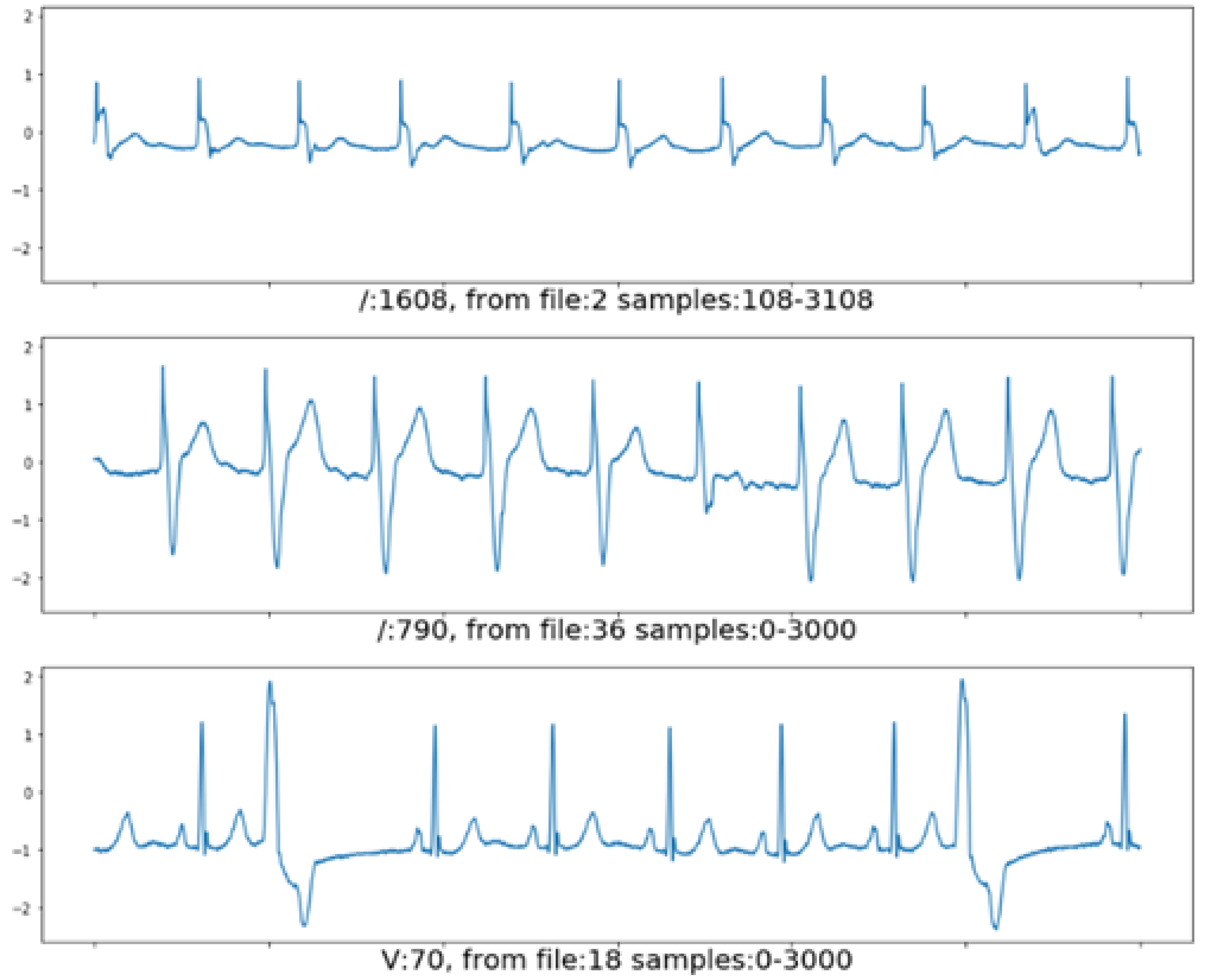
Figure 1 shows examples of ECG pieces of 3000 samples or 8.33 s from the 2nd, 18th, and 36th records. The RR intervals on ECG chunk from the 2nd and 36th files tend to be uniform, while the RR interval on the ECG chunk from the 18th file looks more diverse. Hence, the R-peak detection and the RR interval measurement affect the beat segmentation process.
In this paper, after R-peak detection, beat segmentation starts from
to
, in which
is the RR-interval right before the detected R-peak, while
is the RR-interval right after the detected R-peak. This automatic segmentation window is necessary to ensure that there is only a single beat or R-peak in each segment. The maximum number of samples taken for each segment is 256 points which is equivalent to a duration of 256/360 s or 711 ms. The MIT-BIH database used a sampling rate of 360 Hz, so the 256 sample segment size will be more than adequate as the typical RR interval is around 500 ms [
42].
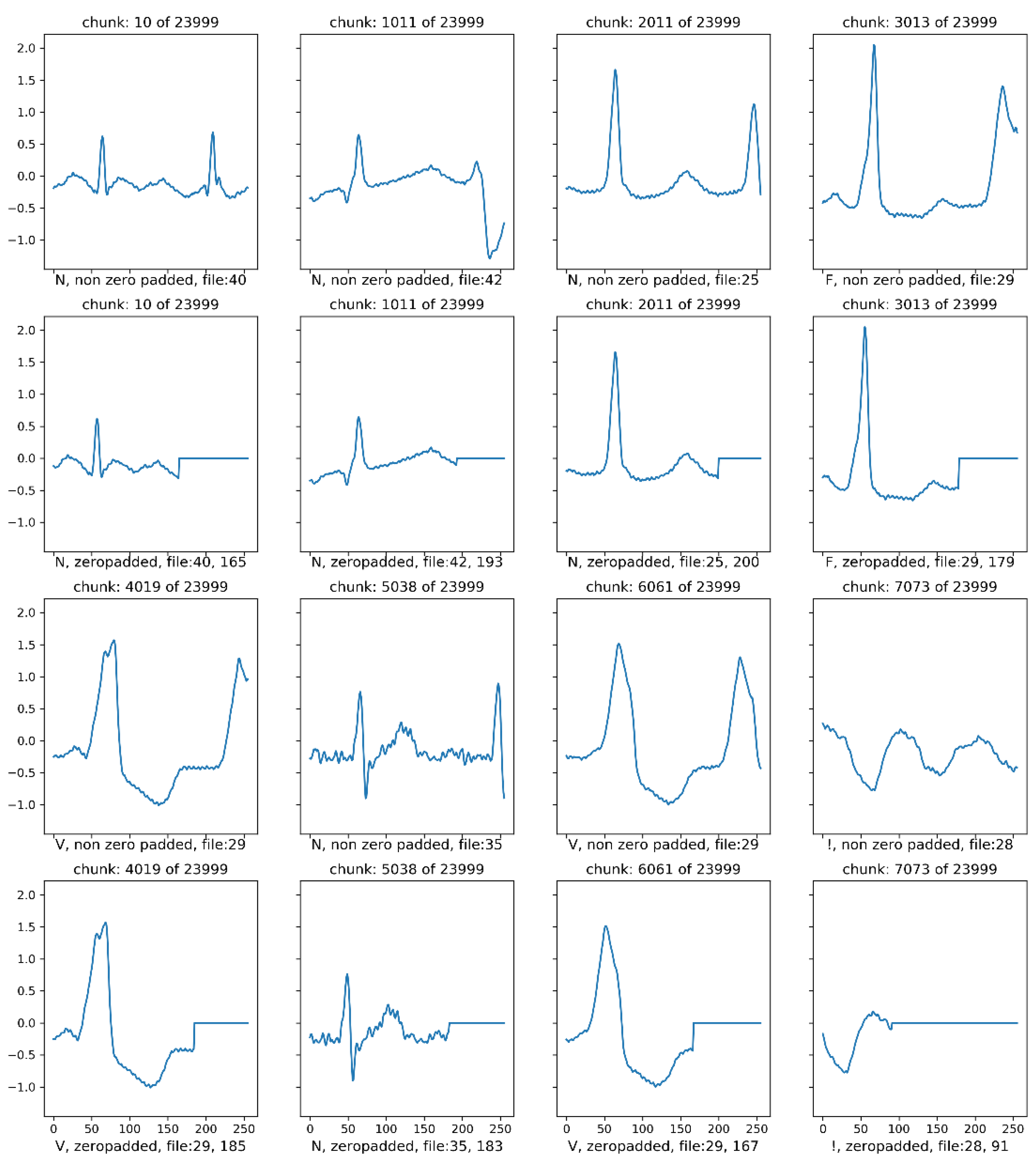
Figure 2 shows the example of our proposed automatic beat segmentation. In our segmentation method, if the RR-interval is too short, or there is more than one R-peak at the segment, then zero- paddings are performed to keep the segment size to 256 samples with only one R-peak. If required, this segment size could be downsampled to 128 or even 64 samples to further reduce the computational cost. However, there will be a slight decrease in the classification accuracy. More experiments are conducted on the sample sizes and its accuracy in the next section.
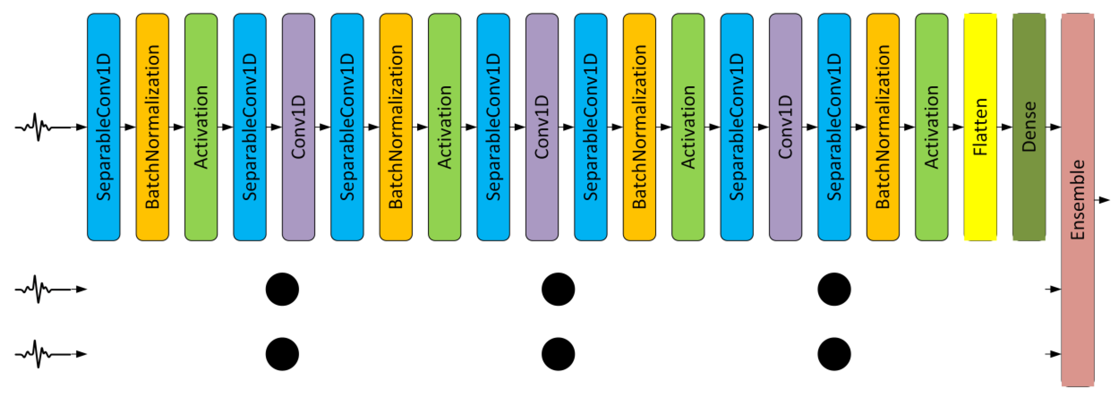
3.2. Ensemble CNNs
Each segmented ECG beat can be replicated into three beat sizes, i.e., 64, 128, and 256 samples. The 64 and 128 samples were the downsampled version of the original 256 beats segmented automatically as explained in
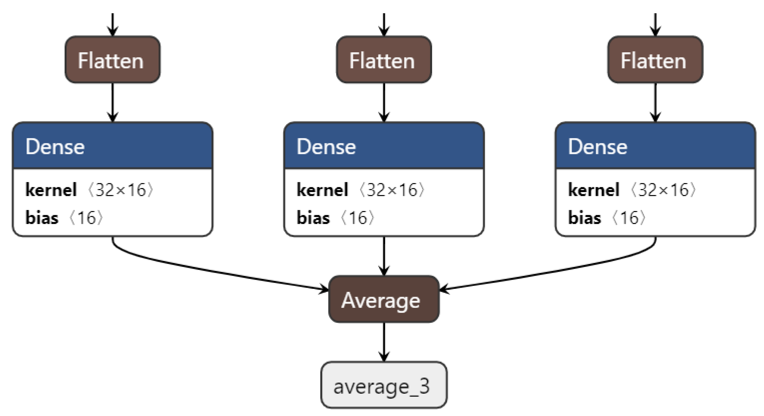
Section 3.1. In total, we have three CNN configurations with a difference only in layer 1 (input size), i.e., 64, 128, and 256. After the training and testing phase, the three outputs from three CNNs were ensembled using the averaging method.
Using ensemble CNN by averaging, it can improve further the accuracy by reducing the variance [
33]. In our proposed algorithm, we calculate the average of all tensor SoftMax from 3 CNNs as shown in Equation (13) and
Figure 3. Let
denote the last layer of the CNN model, and
is the output of
-th neuron at the output layer, and let
denotes the number of CNNs to be ensembled. The final output of the ensemble CNN using averaging can be calculated as follows:
6. Conclusions
In this paper, we presented an efficient algorithm for cardiac arrhythmia classification using the ensemble of depthwise separable convolutional neural networks. First, we optimized the beat segmentation by taking ECG samples centered around the R-peak. Second, we used all convolutional network, batch normalization, and depthwise separable convolution, to achieve the best accuracy while reducing the computational cost. Finally, we ensembled three depthwise separable CNNs by averaging three CNNs of 256 sample input size. Performance evaluation showed that our proposed algorithms achieved around 99.88% accuracy in 16 classes classification. The proposed two-stage ECG classification required around 180 μs, which can be implemented in a real time application. Future work will include the implementation of the current CNN on GPU to speed up its training, as well as to vary the input segment for various patients, the use of different databases, the use of other optimization methods, and the implementation in clinical application validated by a cardiologist.


