3D Dense Separated Convolution Module for Volumetric Medical Image Analysis

Abstract

With the thriving of deep learning, 3D convolutional neural networks have become a popular choice in volumetric image analysis due to their impressive 3D context mining ability. However, the 3D convolutional kernels will introduce a significant increase in the amount of trainable parameters. Considering the training data are often limited in biomedical tasks, a trade-off has to be made between model size and its representational power. To address this concern, in this paper, we propose a novel 3D Dense Separated Convolution (3D-DSC) module to replace the original 3D convolutional kernels. The 3D-DSC module is constructed by a series of densely connected 1D filters. The decomposition of 3D kernel into 1D filters reduces the risk of overfitting by removing the redundancy of 3D kernels in a topologically constrained manner, while providing the infrastructure for deepening the network. By further introducing nonlinear layers and dense connections between 1D filters, the network’s representational power can be significantly improved while maintaining a compact architecture. We demonstrate the superiority of 3D-DSC on volumetric medical image classification and segmentation, which are two challenging tasks often encountered in biomedical image computing.

1. Introduction

During the last few years, Deep Learning (DL) and especially Convolutional Neural Networks (CNNs) have revolutionized computer vision and set new standards for various challenging tasks, such as image classification and semantic segmentation. Since these tasks are also shared in diagnostics, pathology, high-throughput screening, cellular and molecular image analysing and more, the thriving of deep learning was also witnessed in the field of biomedical image analysis [1,2].

However, compared to 2D images mostly used in computer vision, image data encountered in the biomedical field are often volumetric. The substantial difficulties in annotating and interpreting of these 3D volumetric data generally result in a much smaller training set than that of computer vision tasks. In addition, in order to explore the 3D context information effectively, which is essential in volumetric data analysing, much effort has to be made in the designing of the network. The current efforts often lead to either a significant increase in the amount of learnable parameters or the complexity in the network design and training. When dealing with large 3D image volumes, the computational cost, as well as the memory requirement will also become damaging even with cutting-edge computational hardware. Therefore, how to explore the 3D contextual information effectively and train an efficient volumetric network with limited training data are still open problems in the biomedical image computing community.

In order to process 3D volumes using CNNs, many schemes have been proposed in the past few years. One straightforward solution is to apply the conventional 2D CNNs on each volume slice separately [3]. Apparently, this method is a non-optimal use of the volumetric data since the contextual information along the third dimension is disregarded. To make a better use of the 3D context, the tri-planer schemes [4] suggested applying 2D CNNs on three orthogonal planes (i.e., xy, xz and yz planes). Since the inter-slice information is utilized through a selective choosing of input data, only a small fraction of 3D information is explored [5]. By viewing the adjacent volume slices as a time series, the Recurrent Neural Network (RNN) was adopted to distil the 3D context from a sequence of abstracted 2D context [6]. Due to the asymmetric nature of network design, the intra- and inter-slice information cannot be treated and explored equally.

Currently, the 3D CNNs that take 3D convolution kernels as the basic unit [7,8] and their hybrid with 2D CNNs [9] have become the most popular choices in volumetric networks’ design. In addition to impressive 3D context mining ability, the popularity of 3D CNNs is also due to the simple structure nature of 3D operations (e.g., 3D convolutions, 3D pooling and 3D up-convolutions) and their similar usage to corresponding 2D operations [2,8]. As a commonly adopted strategy, a 3D CNN can be constructed from the modern 2D CNNs by replacing the 2D operations with their 3D counterparts.

However, the utilization of 3D operations, especially the 3D convolutional kernels, will introduce a huge increase in the amount of trainable parameters, as well as significant memory and computational requirements [10]. Considering the limited training data often encountered in biomedical tasks, to avoid overfitting, a trade-off has to be made between the scale of the network and its representational power. With these limitations, the existing 3D CNNs tend to contain much fewer layers than modern 2D CNNs in computer vision tasks. For example, 3D U-net has 10 convolutional layers in the encoder part, whereas ResNet [11] usually has 101 convolutional layers. Since the impact of the network’s depth has been extensively demonstrated to produce improved results in computer vision [11,12], there was still much room to explore the potential of 3D CNNs and improve their representational power.

In this paper, instead of modifying the network’s overall architecture to circumvent the trade-off between model size and its representational power, we address this dilemma by looking into the very basic unit of 3D CNNs: 3D convolutional kernels, and propose replacing them with a compact module that possesses better parameter efficiency and stronger nonlinear representational power. We named the proposed module 3D Dense Separated Convolution (3D-DSC), and Figure 1 illustrates its layout schematically.

The 3D-DSC module was constructed by a series of densely connected 1D filters. Decomposing 3D kernels into 1D filters alleviated the risk of overfitting by removing the redundancy within 3D kernels in a topologically constrained manner, while providing the infrastructure for deepening the network. The nonlinear layers inserted between 1D filters were responsible for the boosting of the block’s nonlinearity, as well as its representational power. The dense connections between 1D filters ensured efficient propagation of information and gradient flow, thus facilitating the training of deepened network. Finally, the 1 × 1 × 1 convolution attached at the end of the block acted as a bottleneck layer to reduce the number of output feature volumes. Compared with direct 3D convolutions, the introduction of 3D-DSC not only effectively deepened the network, thus improving its representational power, but also considerably reduced the number of learnable parameters. This feature is especially useful when training data are limited. In addition, since 3D-DSC did not change the number of input and output feature maps of the convolutional layers, it could be directly used to replace 3D convolutions to boost the network’s performance without modifying its overall architecture.

We evaluated the effectiveness and efficiency of 3D-DSC on volumetric image classification and segmentation, which are two challenging tasks often encountered in biomedical image computing. The results on both tasks showed that significant performance improvements could be consistently obtained with comparable or even fewer parameters than the original 3D convolution version.

Our main contributions are summarized as follows.

(1) We propose an effective strategy for alleviating the overfitting problem while enabling the effective training of a much deeper network in volumetric image analysis, especially for the cases with limited training samples. It is demonstrated that a significant accuracy improvement can be achieved in both classification and segmentation tasks with a similar number of parameters.

(2) The dense connections are introduced between 1D filters in our work to facilitate the training of the deeper network, while it is impractical to introduce dense connections for paralleled 2D and 1D filters. In addition, with nonlinear layers inserted, the effective depth of the network, as well as its representational power can be considerably increased without increasing the number of parameters.

(3) The proposed 3D-DSC is not limited to any specific architecture or application, and it can be used to boost the performance by directly substituting the original 3D convolutional kernels.

2. Related Work

Maximizing the potential of training data is a major goal of supervised machine learning. Reviewing the development of deep learning, the pursuit of this goal can be divided into two intertwined stages: the first one aims to build and train deeper networks to digest more data; the second one tries to further mine the potential of given data by improving the network’s parameter efficiency. As the depth of the network in computer vision has becomes saturated, research focusing on exploring network redundancy and designing a more compact architecture has received more attention recently. To the best of our knowledge, in biomedical image computing, there is still little systematic effort dedicated to the reduction of the network’s redundancy. The present work relies heavily on the following two aspects of efforts to reduce parameter redundancy in the field of computer vision.

Many works resort to exploring the redundancy of the network in a post-processing manner. Among these efforts, the Low Rank Approximation (LRA) methods are most relevant to ours. By viewing the convolutional layers as high order tensors, these methods compress the convolutional layers of pre-trained networks by finding their appropriate LRA. Using low rank decomposition to accelerate convolution was first suggested by [13] in codebook learning. In the context of CNNs, the work in [14] proposed a Canonical Polyadic (CP) decomposition and clustering scheme for the convolutional kernels. Pre-trained 3D filters are approximated by consecutive 1D filters, and the error is minimized by using clustering and post-training. The work in [15] suggested using different tensor decomposition schemes, and an iterative scheme was employed to get an approximate local solution. The work in [16] further extended the use of CP decomposition and proposed a different low rank architecture that enabled both approximating an already trained network and training from scratch.

Rather than designing an LRA method, another group of works aimed to improve parameter efficiency. In [17], a spatial separation of the convolution operator was proposed, where the 3 × 3 kernels were separated into two consecutive kernels of shapes 3 × 1 and 1 × 3. Jin et al. [18] exploited structural constraints to conventional 3D CNNs (including channel and spatial dimensions) to reduce the computational cost via separable convolutions. To speed up the computation and reduce the model size, Gonda et al. [19] proposed a novel strategy via replacing 3D convolution layers with pairs of 2D and 1D convolution layers. Numerous other attempts on depthwise separable convolutions have been made in various fashions to improve the efficiency of convolution [20,21,22]. Zhang et al. [23] combined depthwise separable convolution and spatial separable convolution for liver tumour segmentation. In this paper, we separate 3D kernels into 1D kernels, and

Table 1. General comparison with other related methods. LRA, Low Rank Approximation.

Method	Structure	Domain
[17]	2D to 1D	general image
[18]	2D to 1D, depthwise separation	general image
[20,21,22]	depthwise separation	general image
[13,14,15,16]	fine tune the trained model (LRA)	general image
[19,23]	3D to 2D + 1D	medical image
3D-DSC	3D to 1D	medical image

shows the comparison with other relevant methods.

3. Methods

We start this section by discussing the separability of 3D convolutional kernels and the issues that may arise. Then, based on the infrastructure provided by the spatial decomposition of kernels, we construct the proposed 3D-DSC module that possesses better parameter efficiency and stronger nonlinear representational power.

3.1. 3D Separability of Convolutional Kernels

Given a volumetric image, when we employ a 3D convolution kernel to generate a 3D feature volume, the input to the network is the entire volumetric data. By leveraging the kernel sharing across all three dimensions, the network can take full advantage of the volumetric contextual information. Generally, the following equation formulates the exploited 3D convolution operation with stride one in an element-wise fashion:

$$V_{jk}^l(x,y,z)=\sum _{x^{\prime }=1}^X\sum _{y^{\prime }=1}^Y\sum _{z^{\prime }=1}^Z{F}_k^{l-1}(x-x^{\prime },y-y^{\prime },z-z^{\prime })\times W_{jk}^l(x^{\prime },y^{\prime },z^{\prime })$$

(1)

where $W_{jk}^l$ is the 3D kernel of size $X\times Y\times Z$ in the lth layer, which is connected to the kth input feature volume $F_k^{l-1}$ in the previous layer, and the jth output feature volume $F_j^l$, $W_{jk}^l(x^{\prime },y^{\prime },z^{\prime })$ is the element-wise value of the 3D convolution kernel. Assume the lth layer has K input feature volumes, and let $\sigma (·)$ denote the element-wise nonlinear activation function and $b_j^l$ the corresponding bias term; the output feature volume $F_j^l$ is obtained as:

$$F_j^l=\sigma (\sum _{k=1}^K{V}_{jk}^l+b_j^l)$$

(2)

Mathematically, the 3D kernel tensor $W_{jk}^l$ can be factorized into a linear combination of rank 1 tensors according to the CP decomposition:

$$W_{jk}^l=\sum _{r=1}^R{a}_{jkr}^l\otimes b_{jkr}^l\otimes c_{jkr}^l$$

(3)

where R is the rank of $W_{jk}^l$, ⊗ denotes the outer product operation and $a_{jkr}^l\in {\mathbb{R}}^X$, $b_{jkr}^l\in {\mathbb{R}}^Y$, $c_{jkr}^l\in {\mathbb{R}}^z$ are 1D vectors. Element-wise, the above equation can be rewritten as:

$$W_{jk}^l(x,y,z)=\sum _{r=1}^R{a}_{jkr}^l(x)b_{jkr}^l(y)c_{jkr}^l(z)$$

(4)

Substituting (4) into (1) gives the following equivalent expression for the evaluation of the 3D convolution:

$$V_{jk}^l(x,y,z)=\sum _{r=1}^R(\sum _{z^{\prime }=1}^Z(\sum _{y^{\prime }=1}^Y(\sum _{x^{\prime }=1}^X{F}_k^{l-1}(x-x^{\prime },y-y^{\prime },z-z^{\prime })a_{jkr}^l(x^{\prime }))b_{jkr}^l(y^{\prime }))c_{jkr}^l(z^{\prime }))$$

(5)

With this formulation, the 3D convolution can be recast as a sequence of 1D convolutions. From inside out, the calculation within the parentheses can be viewed as: first convolve the feature volume with a 1D filter $a_{jkr}^l$ along the X dimension, then followed by the 1D convolution with $b_{jkr}^l$ and $c_{jkr}^l$ along the Y and Z dimension successively. Vectors $a_{jkr}^l$, $b_{jkr}^l$ and $c_{jkr}^l$ can be viewed as the corresponding horizontal (H), vertical (V) and lateral (L) 1D filters, respectively.

Assuming that the rank of kernel tensor $W_{jk}^l$ is equal to one (i.e., R = 1), the 3D convolution can be decomposed into a sequence of three 1D convolutions as shown in Figure 2 ($R=1$). Note that convolution is a linear operator, and the 1D filters as shown in Figure 1 can be arranged in any order.

Rank 1 is a strong assumption, and the intrinsic rank of $W_{jk}^l$ is generally higher than one in practice, however, the generalization from the rank 1 topology to the rank R case is straightforward. Equation (3) shows that the rank R tensor is the sum of R rank 1 tensors, and this suggested that the rank R topology can be constructed by simply concatenating R copies of the rank 1 topology, as shown in Figure 2 [24].

3.2. 3D Dense Separated Convolution Module

Although the 3D separated convolution topology described in the previous section is mathematically equivalent to direct 3D convolution, the profits of this decomposition are reflected in the following aspects:

First, the rank constraints of 3D convolution kernels can be easily encoded in the network’s topology by stacking k ($k<R$) groups of horizontal, vertical and lateral (HVL) 1D convolutions (as seen in Figure 2). Once the model structure is defined, we can leverage the traditional CNN training method to learn more compact weights from scratch, thus avoiding the traditional post-processing stage of applying the low rank constraint on the pre-trained network, then followed by the iterative fine tuning of layers. In addition, the possible information loss and performance degradation caused by low rank constraints can be minimized as a whole upon training. We will show that the precision can even be increased in the Experiments Section.

Second, when a rank k topology is applied to replace the original full rank 3D convolution kernel, the number of independent parameters per-filter can be reduced from $X\times Y\times Z$ to $(X+Y+Z)\times k$, which results in a significant reduction of the overall learnable parameters for small k considering the huge number of filters deployed in the network. Since the training data size in many biomedical tasks is much smaller than that of computer vision, this reduction in the amount of parameters will reduce the risk of overfitting during training and enable deeper network design.

Finally, the cascaded 1D convolution structure provides the possibility to further improve the nonlinear representation capability of the network. Since the linear combination of convolution operations is still linear, the current decomposed topology can only increase the network’s visual depth, but not the effective depth. However, with this structure, the effective depth of the network can be easily increased by inserting the nonlinear activation layers (e.g., leaky ReLU layers) between the concatenated 1D convolutions, thus increasing the nonlinearity of the network and encouraging the learning of more discriminative features.

However, there are two issues inherited in this kernel decomposition. First, the serialized model with 1D convolutions is more vulnerable to the vanishing gradient problem than standard 3D CNNs. Accompanied by the increase of the network’s depth, longer gradient propagation paths may result in fast gradient decaying, as well as difficulty in optimization. Second, once the nonlinear activation layer is inserted between the 1D filters, the different ordering of the 1D filters will no longer be equivalent.

Inspired by the recent success of densely connected networks [25], we propose to extend the 3D separated convolution discussed in the previous section by further introducing dense connections between 1D filters. Figure 1 illustrates the layout of the rank R 3D-DSC module schematically.

Similar to the DenseNet, we introduce direct connections from any layer to all subsequent layers within each block. In order to maximize the information flow, the features are concatenated and then followed by a composited operations including Batch Normalization (BN) and leaky Rectified Linear Units (leaky ReLU) before they are passed to the next layer. Although each 1D decomposed convolution layer has less parameters, it typically has more input feature maps due to the dense concatenation. It was demonstrated that a 1 × 1 convolution can be employed as a bottleneck layer before each 3 × 3 convolution to reduce the number of input channels [11,25]. To reduce the parameters of 3D-DSC, in this study, we added a 1 × 1 × 1 convolution in each 1D decomposed convolution. In our implementation, we restricted each layer to produce half the number of feature maps as the input. Assume there are k feature maps in the input layer; the concatenate operation after the last 1D decomposed convolution layer will accumulate the feature map to the number of $\frac{5}{2}k$. In order to make the number of output feature maps consistent with that of direct 3D convolution, we introduced an additional bottleneck layer consisting 1 × 1 × 1 convolution after the last 1D convolution layer. With this design, the extension from rank 1 3D-DSC to the rank k case will be the same as the naive 3D separated convolution version, as discussed in the previous section, i.e., by simply stacking k copies of the rank 1 topology.

By introducing the within block dense connections, each 1D kernel is provided with the opportunity to access the input feature map directly, thus to some extent alleviating the ordering problem of 1D kernels. In addition, the employment of dense connections also brings the three following benefits that relieve our previous concerns in a precise manner. First, direct connections between all layers help improve the flow of information and gradients through the network, alleviating the problem of the vanishing gradient. Second, short paths to all the feature maps in the architecture introduce an implicit deep supervision. Third, dense connections have a regularizing effect, and considering the reduction in the number of learnable parameters introduced by 3D separated convolution, such a joint effort would substantially reduce the risk of overfitting under limited training data, which is an essential problem for most biomedical image analysis applications.

Since the size and the number of feature map of our 3D-DSC block are consistent with that of direct 3D convolution, we can directly substitute the 3D convolution layers with 3D-DSC in the existing 2D CNNs and enjoy the benefits of 3D-DSC. If using a high level library such as Keras or TensorFlow-Slim, it would take only several lines of code.

3.3. 3D CNN Architecture Based on 3D-DSC

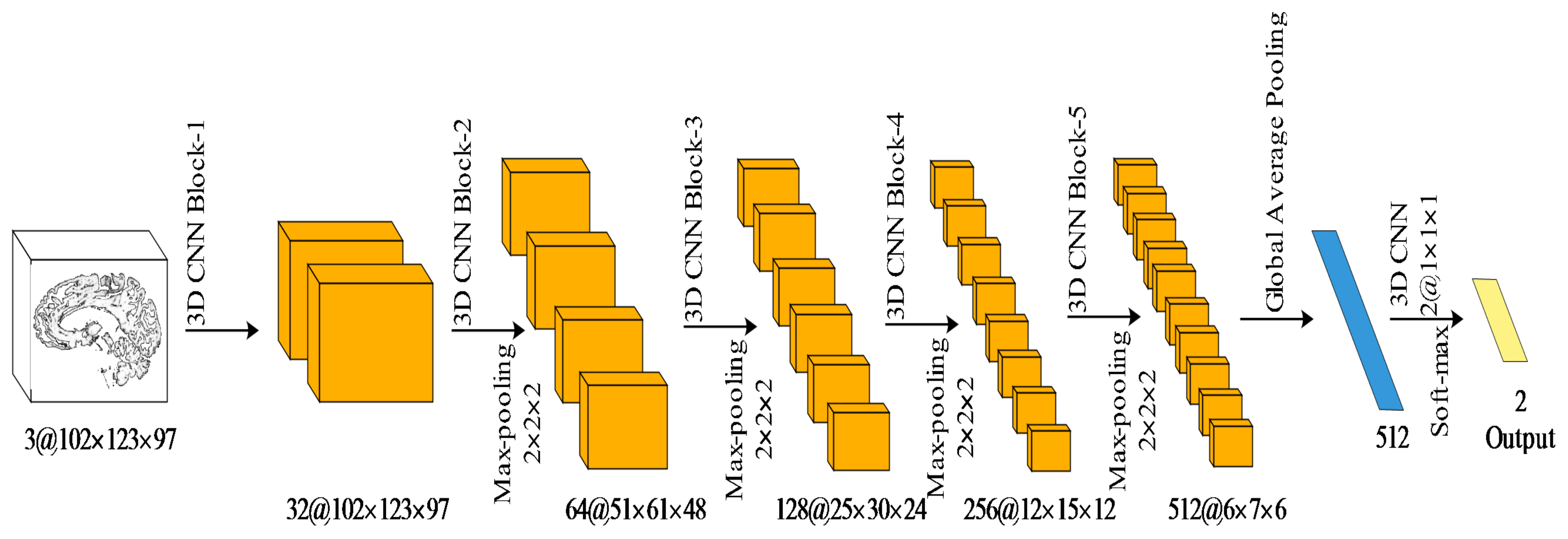
For the classification task, we constructed a simple 3D CNN architecture to diagnose attention deficit hyperactivity disorder. Figure 3 demonstrates the proposed CNN architecture. The architecture followed the typical design philosophy of a convolutional network. It consisted of the repeated application of the 3D convolutional blocks (

Table 2. Architecture overview (shown in columns). $A_n$ are the networks with normal 3D convolution; $B_n$ and $C_n$ are the networks with 3D-DSC; and n represents the number of the additional convolution layers. The 3D convolutional kernel parameters are expressed as “3D-conv 〈kernel size〉/3D-DSC-〈number of output channel〉”. The leaky ReLU activation layer and batch normalization layer are not shown here for brevity.

${\mathit{A}}_{\mathit{n}}$	${\mathit{B}}_{\mathit{n}}$	${\mathit{C}}_{\mathit{n}}$
Input (3D multi-channel MRI)
3D-conv3-32	3D-conv3-32	3D-conv3-32
3D-conv3-32	3D-conv3-32	3D-conv3-32
Max pooling
3D-conv3-64	3D-conv3-64	3D-conv3-64
3D-conv3-64	3D-conv3-64	3D-DSC-64
Max pooling
3D-conv3-128	3D-conv3-128	3D-conv3-128
3D-conv3-128 $\times n$	3D-DSC-128 $\times n$	3D-DSC-128 $\times n$
Max pooling
3D-conv3-256	3D-conv3-256	3D-conv3-256
3D-conv3-256 $\times n$	3D-DSC-256 $\times n$	3D-DSC-256 $\times n$
Max pooling
3D-conv3-512	3D-conv3-512	3D-conv3-512
3D-conv3-512 $\times n$	3D-DSC-512 $\times n$	3D-DSC-512 $\times n$
Global Average Pooling
3D-conv1-2
Softmax

shows the number and the type of 3D convolutions in each block), each followed by a $2\times 2\times 2$ 3D max pooling operation with stride 2 for downsampling. After each downsampling layer, we doubled the number of volumetric feature channels. At the final layer, a 3D global average pooling and a $1\times 1\times 1$ 3D convolution were used to map each volumetric feature vector to the desired number of classes.

For the segmentation task, we applied the classic 3D U-net architecture. We kept the typical encoder-decoder structure and the number of blocks in each path. Different from the original 3D U-net, we used instance normalization and leaky ReLUs, rather than batch normalization and ReLUs. Based on these, we designed a universal 3D U-net block with 3D-DSC. Figure 4 shows the proposed 3D U-net block. The block reserves the first normal 3D convolution, followed by 2 3D-DSC.

3.4. Training of the 3D CNN Architecture

Both classification and segmentation CNNs were trained end-to-end on the datasets of brain scans in MRI. An example of the typical content of such volumetric medical image is shown in Figure 5.

In this paper, we select the cross-entropy as the classification loss function and the Dice loss as the segmentation loss function. The cross-entropy $CE$ can be written as:

$$CE=-\frac{1}{N}(\sum _{n=1}^N{y}_{n}lnH(x_n)+(1-y_n)ln(1-H(x_n)))$$

(6)

where N is the number of samples, $x_n$ and $y_n$ are the input and corresponding label of the nth sample, $H(·)$ is the function learned by the network and $H(x_n)$ represents the output of the neural network given the input $x_n$. The Dice loss D for binary classes is defined as follows:

$$D=\frac{2{\sum }_i^N{p}_i{q}_i}{{\sum }_i^N{p}_i^2+{\sum }_i^N{q}_i^2}$$

(7)

where the sums run over the N voxels, of the predicted segmentation volume $p_i\in P$ and the ground truth volume $q_i\in Q$.

We employed a similar training strategy during classification and segmentation. It is worth noting that adaptive optimization methods have better performance in the early stage of training, but are outperformed by Stochastic Gradient Descent (SGD) at later stages. To minimize the effect of random initialization, we firstly trained the model with random initialization and the Adam [28] optimizer. Then, we refined the model with the SGD optimizer. The learning rate was initially set to 0.00001 and decreased by a factor of 10 when the validation error stopped decreasing. The early-stopping strategy was used with patience of 50. We denote the mean difference between the training loss and the validation loss within the last 50 epochs as the Overfitting Distance (OD), which can be used to evaluate the ability of the network to cope with overfitting. The OD can be written as:

$$OD=\frac{1}{N}\sum _{i=1}^N\left|T_i-V_i\right|$$

(8)

where N is the training epoch numbers, $T_i$ is training loss and $V_i$ is validation loss. In our experiments, we employed 5 fold cross-validation to evaluate the proposed method.

4. Experiments and Results

In this section, we evaluate the proposed module on two different volumetric image analysis tasks (attention deficit hyperactivity disorder diagnosis and brain tumour segmentation) with a comparison to several state-of-the-art methods. In addition to the precision evaluation, the components, depth and overfitting analyses are also provided to illustrate the effectiveness and superiority of our method.

4.1. Attention Deficit Hyperactivity Disorder Diagnosis

Attention Deficit Hyperactivity Disorder (ADHD) diagnosis is one of the most common mental health disorders, affecting around 5–10% of school aged children. In order to diagnose this disorder automatically, MR images, including structural MRI (sMRI) and functional MRI (fMRI) have been investigated in many studies. The MRI data analysed in this paper were from the ADHD200 consortium [26,29]. Initially, they posted a large training dataset including 776 samples comprised of 491 typically developing individuals and 285 patients with ADHD. For the ADHD-200 global competition, the ADHD-200 consortium also released a hold-out dataset from 171 subjects, including 94 Typically Developing Children (TDC) and 77 ADHD patients [8]. For each sample, both fMRI scans and associated T1 weighted structural scans were provided. With the R-fMRI Maps Project, Chaogan et al. processed the MRI dataset and provided three kinds of voxel based morphometric features, including Grey Matter (GM), White Matter (WM) and Cerebrospinal Fluid (CSF), and three kinds of features from fMRI scans, including Regional Homogeneity (ReHo), fractional Amplitude of Low Frequency Fluctuations (fALFF) and Voxel Mirrored Homotopic Connectivity (VMHC) in [30]. In our experiment, these features were regarded as three individual input channels of network.

4.1.1. Network Architecture

Table 2 shows the configurations of the baseline models ($A_n$) and their 3D-DSC enhanced versions ($B_n$ and $C_n$). All networks started with two 3D convolutional layers and one pooling layer. The difference between $B_n$ and $C_n$ was whether 3D-DSC modules were used or not between the first two pooling layers. Starting from the second max pooling layer, both $B_n$ and $C_n$ were constructed by repeating a combination of one 3D convolution layer, n 3D-DSC layers and one pooling layer where the first 3D convolution layer acted as the transition layer [25]. Then, the global average pooling layer and $1\times 1\times 1$ convolution were applied on the feature volumes, and softmax was employed as the last layer for classification.

4.1.2. Accuracy and Analysis of the Network’s Depth

It is well known that the depth of a network has a big impact on its performance.

Table 3. Performance comparison based on 5 fold cross-validation. $A_0$∼$A_6$ are normal 3D CNNs with different depths. $B_1$∼$B_6$ and $C_6$ are the separated 3D CNNs with 3D-DSC. OD denotes the Overfitting Distance. The batch size is 4 in this experiment.

Network	Depth	Params	Accuracy	OD
$A_0$	8	4.8 M	73.17%	0.2785
$A_1$	11	14.1 M	74.89%	0.2806
$A_2$	14	23.4 M	74.53%	0.2807
$A_3$	17	32.7 M	71.94%	0.2961
$A_4$	20	42.0 M	70.78%	0.3368
$A_5$	23	51.3 M	69.91%	0.3390
$A_6$	26	60.6 M	69.22%	0.3567
$B_1$	11	7.2 M	73.45%	0.2415
$B_2$	14	9.6 M	74.58%	0.2498
$B_3$	17	12.1 M	75.22%	0.2526
$B_4$	20	14.4 M	75.57%	0.2610
$B_5$	23	16.9 M	75.79%	0.2689
$B_6$	26	19.3 M	75.74%	0.2809
$C_6$	26	19.2 M	76.70%	0.2580

shows the accuracy and OD score of networks with different depth configurations. For the baseline method ($A_n$), we can see that $A_1$ achieved the best result. However, its performance would deteriorate as we deepened the networks. We believe that the aggravation of overfitting was responsible for this degradation since the number of parameters would increase dramatically with a deeper network. As shown in the third column of Table 3, from $A_0$ to $A_6$, the number of parameters increased from 4.8 M to 60.6 M. As the number of tunable parameters increased, the models tended to be more susceptible to overfitting, resulting in the severe deterioration of the OD score, as well as the performance. While in $B_n$ and $C_n$, since the 3D convolutions were replaced by parameter efficient 3D-DSC modules, considerable parameters could be reduced, and more parameter space was made available for designing deeper networks.

Note that $B_4$ and $A_1$ have a similar number of parameters, but the effective depth of $B_4$ increased from 11 layers to 20 layers; thus, more representation power could be expected. In Table 3, a stable accuracy improvement of $B_1$ to $B_5$ can be observed. In addition, we can notice that the OD scores of $B_4$ and $B_5$ were both smaller than $A_1$, which further validated that our method could better handle the risk of overfitting. Another example that could verify the performance of our method was $C_6$. We can see that $B_5$ achieved the best performance in $B_n$ networks, and the performance and OD score of $B_6$ already showed the trend of degradation. As shown in Table 2, $C_6$ replaced one more layer with 3D-DSC than $B_6$ (between the first two pooling layers); therefore, $C_6$ had the same depth as $B_6$, but it had less parameters and a stronger ability to avoid overfitting. We can see that $C_6$ achieved the highest accuracy among all networks, and its OD score was smaller than $B_6$. Although deeper networks might provide better performance, we could not continue to deepen the network due to the limit of GPU memory (12 GB of Titan-XP). These results confirmed that deeper networks could be obtained and effectively trained with 3D-DSC, thus improving the network’s representation power. Moreover, as shown in Table 4, compared with several state-of-the-art methods attempting to assist the diagnosis, $C_6$ outperformed the others by a large margin on the ADHD-200 even if only a single modality of the dataset was used in our method.

We attributed the performance improvement of the proposed 3D-DSC based methods to the following two main factors.

(1) The parameter efficient nature of the proposed 3D-DSC made the effective training of deeper network possible while reducing the risk of overfitting. For instance, there were 23.4 M parameters in $A_2$. If we simply increased the depth of the network from $A_2$ to $A_3$, the increased parameters would quickly saturate the network (the accuracy dropped from 74.53% to 71.94% and the overfitting distance raised from 0.2807 to 0.2961). By introducing 3D-DSC, the number of parameters for each 3D kernels was significantly reduced, and we could construct $C_6$ with less parameters and deeper architectures [31]. In addition, the employment of dense connections in the 3D-DSC module further improved the parameter utilization efficiency by encouraging feature reuse.

(2) The stronger nonlinear representation ability was powered by the more activation layers integrated in 3D-DSC. By decomposing the 3D kernel into a series of concatenated 1D filters and inserting activation (nonlinear) layers between them, the effective depth of network, as well as its representational power could be considerably increased without increasing the number of parameters. The normal 3D convolution was usually followed by only one activation layer, whereas each 3D-DSC module could accommodate four or more activation layers. The effect of additional activation layers could also be observed in our ablation studies, as illustrated in

Table 5. Ablation studies for applying Dense Connection (DC) and activation layer (activation for short) in the proposed 3D-DSC. OD: Overfitting Distance. Orders: the orders of separated 1D filters, including H (Horizontal), V (Vertical) and L (Lateral). The batch-size is 4 in this experiment.

Network	DC	Activation	Orders	Accuracy	OD
$B_3$	no	no	H, V, L	74.26%	0.2733
$B_3$	no	yes	H, V, L	74.83%	0.2638
$B_3$	yes	yes	H, V, L	75.22%	0.2526
$B_3$	yes	yes	V, L, H	75.28%	0.2507
$B_3$	yes	yes	L, H, V	75.19%	0.2514

.

Table 4. Diagnosis performance comparisons between the proposed method and state-of-the-art methods based on the ADHD-200 dataset. MKL: Multi-Kernel Learning. SVM: Support Vector Machine. SM: Single Modality. MM: Multiple Modalities. The batch-size is 4 in this experiment.

Method	Classifier	Accuracy
[32]	MKL	61.54%
[33]	SVM	69.62%
[34]	SVM	63.57%
[8]	SM 3D CNN	66.04%
[8]	MM 3D CNN	69.15%
[35]	4D CNN	71.30%
3D-DSC ($C_6$)	SM 3D CNN	73.68%

Table 4. Diagnosis performance comparisons between the proposed method and state-of-the-art methods based on the ADHD-200 dataset. MKL: Multi-Kernel Learning. SVM: Support Vector Machine. SM: Single Modality. MM: Multiple Modalities. The batch-size is 4 in this experiment.

Method	Classifier	Accuracy
[32]	MKL	61.54%
[33]	SVM	69.62%
[34]	SVM	63.57%
[8]	SM 3D CNN	66.04%
[8]	MM 3D CNN	69.15%
[35]	4D CNN	71.30%
3D-DSC ($C_6$)	SM 3D CNN	73.68%

4.1.3. Ablation Studies

To investigate the effect of nonlinear activation layers and dense connections inserted between the separated 1D filters, we report the performances of $B_3$ with and without nonlinear layers and dense connections in Table 5. We can see that both of them contributed to the performance improvement, and the best result could be obtained by a combination of them. B3 networks with different orders provided similar performance. The orders of separated 1D filters hardly influenced the performance of 3D-DSC.

4.1.4. Overfitting

To further confirm the ability of 3D-DSC to cope with overfitting, we compared the performance of the baseline method with ours by removing the Batch Normalization (BN) layers. For demonstration purposes, we set the batch size to one to highlight the effect of the 3D-DSC module. The learning rate was initially set to 0.0001. Figure 6 shows the loss curve of $A_3$ and $B_3$ (without the BN layer) on the validation dataset. We can see that the validation loss of $A_3$ increased rapidly from 60 epochs, while that of the $B_3$ network remained stable, even after 100 epochs. Furthermore, the OD score of $A_3$ was 0.9962, which was significantly larger than the 0.2946 of $B_3$. Compared with $A_3$, the more compact structure and much less learnable parameters of $B_3$ made it less susceptible to overfitting. Dense connections had several outstanding advantages: strengthen feature propagation, encourage feature reuse, and substantially reduce the number of parameters [25].

4.2. The Brain Tumour Segmentation on BRATS 2017

In this section, we evaluate the proposed method on another challenging task of brain tumour segmentation, using the publicly available dataset of the BRATS 2017 challenge [36]. The training dataset contained 285 multi-sequence MRIs of patients diagnosed with low grade gliomas or high grade gliomas. In each case, four MR sequences were available: T1, T1 + gadolinium, T2, and Fluid Attenuated Inversion Recovery (FLAIR). In this study, we employed these multi-modality MRI scans to segment the gliomas, neglecting the difference between oedema, necrosis and non-enhancing tumour, as well as enhancing tumour (i.e., binary classification). We resized all volumes to $(64\times 64\times 64)$, and four MRI sequences for each sample were combined as a multichannel volume as input. Three competitive methods including 3D U-net [37] (along with its dropout and stride two convolution enhanced versions), V-net [38] and the method proposed in [39] were evaluated and compared.

The five fold cross-validation strategy was employed in this experiment. In each iteration, one fold with 57 samples was used for testing, and the rest were used for training the model. This process was repeated five times until each of these five folds had been used as the testing set. To illustrate the effectiveness of the proposed 3D-DSC module, we replaced the original 3D U-net block as shown in Figure 4a with our 3D-DSC enhanced version as shown in Figure 4b and compared the performance with/out 3D-DSC. Note that only the second 3D convolution in 3D U-net was substituted by two consecutive 3D-DSC modules, and the overall architecture of the network remained unchanged. The Dice scores obtained by different methods are shown in

Table 6. The experimental results of the proposed method and state-of-the-art methods. We trained and evaluated these methods with the same strategy on the BRATS 2017 dataset. s2, stride 2.

Method	Depth	Params	Dice Score
3D U-net	19	23.5M	0.8554
3D U-net (Dropout)	19	23.5 M	0.8592
3D U-net (s2-conv)	23	25.9 M	0.8593
[39]	23	25.9 M	0.8655
V-net [38]	19	23.5 M	0.8685
3D U-net (3D-DSC)	28	17.8 M	0.8932

. We can see that our method achieved the best performance with a Dice score of 0.8932, which outperformed the others by a large margin. It is worth noting that we did not adopt any other technique to refine the network, such as dropout, replacing pooling with stride two convolution (s2-conv), and so on, although these techniques could slightly improve the performance of 3D U-net as reported in Table 6. The qualitative segmentation results of different methods are presented in Figure 7, and we can see that fine details could be better recovered by our method. Even though the performance reported here did not represent the state-of-the-art performance on BRATS 2017 [40], it demonstrated that replacing the 3D convolution kernels by the proposed 3D-DSC was able to reduce the risk of overfitting and hence improve the performance via a deeper network.

5. Conclusions and Discussion

The effective and efficient exploration of 3D contextual information is essential in volumetric data analysis. Although the performance of CNNs in 2D image analysis is impressive, the predictive power of its 3D generalization (i.e., 3D CNNs) is always constrained by the number of samples, especially in biomedical image analysis. Considering the conflict between the huge amount of parameters to learn in 3D CNNs and limited training samples that would quickly lead to overfitting, in this paper, we proposed a novel 3D-DSC module to replace the traditional 3D convolutional kernels. The proposed 3D-DSC module consisted of a series of densely connected 1D filters. This architecture was able to remove the redundancy within 3D kernels, while providing spaces for deepening the network and therefore could effectively reduce the risk of overfitting. In addition, inspired by the recent success of the residual network and densely connected networks, we extended the 3D separated convolution block by introducing dense connections within and between blocks. The dense connection provided an effective way to combine subsequent layers and facilitated the flow of information. Furthermore, we investigated the effect of nonlinear activation layers between the concatenated 1D filters, which had the potentiality to increase the representational power of the network and facilitate the learning of discriminative features. Experimental results on the ADHD classification and brain tumour segmentation demonstrated the superiority of the proposed 3D-DSC on volumetric image analysis. Note that 3D-DSC was not limited to any specific architecture or application and could be used to boost the performance by directly substituting the original 3D convolutional kernels.