Jet Noise in Airframe Integration and Shielding


Aerospace Engineering Department, Embry-Riddle Aeronautical University, Daytona Beach, FL 32114, USA
*
Authors to whom correspondence should be addressed.
Appl. Sci. 2020, 10(2), 511; https://doi.org/10.3390/app10020511
Submission received: 21 November 2019
/
Revised: 16 December 2019
/
Accepted: 3 January 2020
/
Published: 10 January 2020
(This article belongs to the Special Issue Airframe Noise and Airframe/Propulsion Integration)
Abstract
:This paper reviews and presents new results on the effect of airframe integration and shielding on jet noise. Available experimental data on integration effects are analyzed. The available options for the computation of jet noise are discussed, and a practical numerical approach for the present topic is recommended. Here, it is demonstrated how a hybrid large eddy simulation—unsteady Reynolds-averaged Navier-Stokes approach can be implemented to simulate the effect of shielding on radiated jet noise. This approach provides results consistent with the experiment and suggests a framework for studying more complex geometries involving airframe integration effects.
1. Introduction
The Federal Aviation Administration (FAA) in the U.S. has implemented detailed noise certification requirements in Federal Aviation Regulation (FAR) Part 36 (5) [1]. For instance, the maximum noise levels should not exceed the limit of 108 in effective perceived noise in decibels (EPNdB) during approach and flyover stages. Such limitations have motivated various research efforts to predict and control un-installed engine noise. However, engine noise is modified as a result of the installation on the aircraft. Most subsonic engines now use high bypass ratio configurations, which increases its size and may intensify the installation effects. Therefore, we address here the airframe effects on the radiated noise. Jet noise is a key component of the engine noise and it could be the most affected component due to the airframe integration. Therefore, our focus here is on jet–airframe (J-AF) interactions. Such interactions can modify noise generation and radiation significantly, and if these effects are understood, the interaction with the airframe can even be utilized to minimize noise radiation.
The outline of this paper is as follows: A review of current experimental observations on airframe integration on jet noise is given in Section 2. This is followed by a discussion of jet noise computation techniques in Section 3, including active flow and noise control, as the existing trend toward modifying noise generation. Although there are several experimental data on the installation effect on jet noise, there are very few, if any, large-eddy simulations (LESs) that capture both the flow–structure interaction, as well as the radiated noise. Therefore, a specific flow–structure interaction numerical model is presented to simulate shielding effects in Section 4. This provides a tool for further investigations of the airframe effects in more complex geometries.
2. Experimental Observation on Airframe Effect on Jet Noise
Jet noise can be a crucial factor in the design of future military and high-speed commercial aircraft. Many advanced aircraft concepts are moving towards tighter coupling of propulsion systems with airframe aerodynamics to achieve optimal performance. Such integration can have a significant effect on the noise generated caused by alterations of the flow field. On the other hand, the orientation of the propulsion system with respect to the wing can change the noise propagation due to shielding or reflection of engine noise. In general, the investigation of airframe propulsion aeroacoustics includes both reducing the noise sources that arise from integration, as well as employing the installation itself as an approach to reduce noise of the airframe or propulsion system. For example, current aircraft designs may employ complex geometry exhaust systems to maximize efficiency or reduce noise. The subsonic jet engines have benefited from the large bypass ratio design to reduce noise emission. However, a great part of the research on supersonic aircraft has been focused on minimizing sonic boom. The design criteria stemmed from these efforts have led to embedded engine designs, which often suggests exhaust of jet over aft-airframe surfaces. We review here the effect of propulsion–airframe interactions on jet noise for both conventional aircraft designs, as well as some novel configurations. Installation effects of conventional designs include the wing behaving as a reflective surface, the wing or flap interacting with the exhaust flow, the pylon causing a large fan blockage resulting in an asymmetric flow, or a combination of these effects.
2.1. Jet—Pylon Interactions
When an aircraft engine is mounted to the wing, the engine pylon provides an aerodynamic shape around the rod support that connects the engine’s core housing to the wing structure. In the conventional aircraft designs, where the engine is placed under the wing, installation effects due to the pylon can modify the flow. These asymmetries in the flow field caused by the pylon affect the exhaust plume, and as a result, change the far-field acoustics. In general, the pylon increases the OASPL in the far-field [2].
Bhat [3] carried out experiments on a bypass ratio five separate flow nozzle to measure the effect of the pylon relative to the baseline axisymmetric nozzle. The effect of adding the pylon was found to increase the EPNdB relative to the baseline, from 1 to 3 EPNdB at different power settings. Thomas and Kinzie [4] performed experimental studies to investigate acoustic effects of jet–pylon interaction for separate flow and chevron nozzles of both a bypass ratio five and eight. They concluded that, for the bypass ratio eight configuration, the effect of adding a pylon to the baseline nozzle is to slightly increase the noise for the case with a core chevron. Figure 1 shows the pylon installed on the separate exhaust nozzle, along with the perceived noise level (PNL) directivity.
The model shown in Figure 1a corresponds to an approximate scale factor of nine used in the wind tunnel tests reported in [4]. One of the challenges in these investigations was the existence of several mechanisms responsible for noise generation, and since no specific pylon size or shape exists, it was difficult to quantify the individual mechanisms of noise generation. However, the effects of different pylons on an engine’s exhaust flow are qualitatively similar. These effects include both modifications to the exhaust flow field, as well as acoustic changes due to waves reflecting from surface near the noise sources.
One of the mechanisms responsible for modifications of the flow field due to the presence of the pylon is the deflection of the core flow. The viscous forces of the core stream cause the flow to resist separation from the pylon shelf, and consequently, the core flow is turned upwards toward the pylon. This process is generally known as the “Coanda effect”. The other mechanism that is known as “rooster tail effect” follows this deviation of the core flow. The upward velocity component of the core flow cuts against the fan flow and is sucked to fill the void below the core flow, resulting in two strong counter-rotating vortices shed from the pylon. Figure 2 illustrates both the Coanda effect and the rooster tail effect.
2.2. Jet—Wing Interactions
The reflection and diffraction of the waves emitted from the jet due to the presence of the wing and its high-lift devices can change the flow-acoustic field. Head and Fisher [5] studied the interaction between an unheated single flow free jet and a reflective surface to investigate the augmentation of low frequency noise due to the presence of an acoustically reflective wing. They observed the effect of noise on both low and high frequencies. The low frequency installation effects are due to the near-field edge diffraction of a quadrupole noise source. The high frequency increase has been shown to result from incoherent noise reflection off the lower surface of the wing [6]. Similar results were also obtained by Brown and Ahuja [7].
2.3. Jet—Flap Interactions
The interaction of the exhaust jet and flaps can generate new noise sources, which is mainly known as jet–flap interaction noise. The principal mechanism is believed to be the impact of the downwash of the wing-flap on the jet flow [8,9,10]. Figure 3 illustrates interaction between the jet and wing in the conventional under-the-wing configuration. Generally, the acoustic waves emanated from the jet hit the aerodynamic surfaces, and the reflection of such waves may influence the instability waves near the nozzle as they exit the shear layer and modify the turbulent structure of the jet. Such modifications in the flow field are referred to as new sources of noise that change the perceived noise. Since the real configuration of jet-wing-flap is rather complex, the effect of flaps on the jet is reviewed independently.
Mead and Strange [11] investigated the under-the-wing installation effects on jet noise. They reported the measurement of the high installation noise level in the low frequency range. They carried out experiments under static conditions and the effect of forward flight was not considered. The forward flight effect is extremely important in the interaction between the flow around the wing-flap and the jet. Several investigations were conducted at the Boeing company [12,13,14] to include the effect of forward motion of the aircraft. Bhat [15] studied the sensitivity of installation noise to a range of parameters, such as the wing-flap settings, jet engine location, and pitching angle. The installation effect was reported to increase noise up to 6 dB. Following these experiments, some empirical prediction methods were developed to determine installation noise, such as [14,16]. Since the noise levels were high, many studies focused on reduction technologies. Mengle et al. [17] investigated the effect of chevrons on installed engines. Their experimental results show that the installation effects of chevrons in conventional nozzles are reversed at approach and take-off. This trend is not observed in isolated nozzles. In addition, it was reported that certain azimuthally varying chevrons give larger total installed noise benefits at both conditions compared to conventional chevrons.
Due to the complexity of the installation effects of the jet–flap interactions, some studies have investigated this configuration along with pylon effects. For example, Faranosov et al. [18] performed experiments for a typical swept wing with an installed dual-stream nozzle and removable pylon. The effect of the flap deflection angle on jet–flap interaction noise was studied with and without the pylon for static and flight conditions. These experiments show that for both cases of with and without the pylon, jet–flap interaction noise remains qualitatively the same and is very sensitive to the flap deflection angle for static and flight conditions. However, the intensity of jet–flap interaction noise increases for the full configuration with the pylon installed.
2.4. Hybrid Wing Body Concept
One of the approaches to reduce engine noise by changing propulsion system orientation, is to benefit from configurations, such as in the over-the-wing engine mount in the hybrid wing body (HWB) concept [19]. Early assessments of the HWB noted limited potential for noise reduction, specifically a Boeing version of an HWB called the “blended wing body” of Liebeck et al. [20]. This configuration had the engine exhaust positioned aft of the trailing edge, making shielding of the aft-radiated engine noise sources impossible, unless the engines were moved at least some limited distance upstream on the airframe [21]. Also, various future aircraft design concepts consider over-the-wing engine configurations, in which the wing or any other airframe structures can be used as a shield against engine noise (i.e., [22]). For example, a hybrid wing body configuration under NASA’s N + 2 test [23] enhances the design by moving the engine nacelles forward of the trailing edge to shield the aft turbomachinery and jet noise.
The HWB design has attracted many researchers in the past years to move towards the noise reduction goals of NASA and FAA [24]. From the jet noise reduction perspective, this design mainly relies on the jet shielding [25,26] enhanced by the aft body section, as illustrated in Figure 4. The focus of these experiments was to investigate the shielding effect on the exhaust jet and prospective acoustic mitigation of the aft-body section.
2.5. Shielding Effects
A series of tests [27,28] were conducted at NASA Glenn Research Center in order to study the propulsion–airframe integration under jet–surface interaction tests (JSITs). Bridges [29], and Zaman et al. [30] focused on the noise generation mechanism in subsonic jets, and investigated the effects of the surface length, distance from the nozzle, lip to the trailing edge, and beveled nozzle configurations. Bridges [31] tested rectangular jets of various aspect ratios (ARs) in the proximity of a flat surface. Sample spectra are shown in Figure 5 for a Mach 0.97 unheated rectangular jet () parallel to the plate at a distance of , and plate length of . Measurements are shown at a polar angle of , which represents the microphone location directly above or below the surface, as well as for the isolated jet. The corresponding non-dimensional frequencies are calculated and the Strouhal number, , is shown under the figure. Here, the length scale, , is chosen as the corresponding hydraulic diameter, , and the isentropic jet exit velocity of . Moreover, in an effort towards integration of the airframe with the nozzle design, Bridges [31] investigated the far-field acoustic measurements of a family of high aspect ratio rectangular nozzles in the high subsonic flow regime with various designs. These experiments reported that having an extended lip on one broad side produced up to 3 dB more noise in all directions while extending the lip on the narrow side produced up to 2 dB more noise, primarily on the side with the extension. Adding a non-intrusive chevron made no significant change to the noise while inverting the chevron produced up to a 2 dB increase in the noise.
Regarding the supersonic jet–surface interactions, McLaughlin et al. [32] carried out experimental and numerical studies on a 1.5 Mach jet at various distances from a flat surface and observed that both scrubbing and trailing edge noise detected in low frequencies increased, as the distance between flat plate and the jet is reduced.
Brown et al. [33] and Clem et al. [34] provided flow field and acoustic data for a supersonic round jet with a design Mach number of 1.5, operating in the over-expanded, ideally expanded, and under-expanded supersonic flow regimes. The plate was placed at a radial distance, , normalized by the jet exit diameter, . They tested a range of distances between . For noise testing, the surface was assembled using multiple pieces of 12.7-mm-thick aluminum to allow six surface lengths, , between . For the narrowband spectra shown in Figure 6, the flat plate with a surface length of is located at , and the jet is at the ideally expended operating condition with the design Mach number of . A reduction in broadband shock-associated noise was observed both in the shielded direction, 60° and 90° microphone angles, when the flat surface was long enough to cover the shock cells in the potential core.
Mora et al. [35] tested a supersonic rectangular nozzle of a 2:1 aspect ratio and 1.5 Mach number with and without the plate for various nozzle expansion conditions and documented a range of plate positions where crackle levels were significantly intensified. In their study, the plate could be positioned at different stand-off distances, starting where the plate touches the inner wall of the nozzle exit at and could be moved away from the jet up to .
Figure 7 illustrates the Schlieren images of the free jet and the shielded jets for these studies, where the effect of the shielding plate on the jet is apparent in Figure 7b. Mora et al. [35] reported that and 3 have similar overall sound pressure level (OASPL) compared to the no-plate configuration. The configuration increases noise levels significantly, starting at an angle of 128°. Similar behavior has also been reported by Powers et al. [36]. The acoustic directivity, shown in Figure 8, revealed the shielding effect of the flat plate at various angles.
Following the valuable findings from these experiments, Brown [37,38] created empirical models that can predict acoustic effects for a range of jet flows and surface geometries. Bridges et al. [39] extended the acoustic modeling of jet–surface interaction from simple single stream jets to a realistic dual-stream exhaust nozzle. Moreover, the experimental set up considered the presence of the flight stream around the jet and surface to mimic practical flight conditions.
3. Options for Computation of Jet Noise
Jet noise is produced by the unsteady turbulent fluctuations in the jet. Reynold averaged Navier-Stokes (RANS) can predict turbulence only by means of time-averaged quantiles; the time-averaged quantiles do not directly produce noise, it is the time varying that is required for the calculation of noise. Thus, prior to 1990, the industry relied on empirical formulas for the prediction of engine noise. The success of such an approach is limited, particularly when addressing new designs that include various options for propulsion–airframe integration. We discuss here how jet noise can be calculated with and without the airframe integration effects.
In the 1980s, lacking full computational power, an attempt to calculate the jet noise produced by large eddies was given by Mankbadi and Liu [40]. They modeled large eddies as a wave packet with a radial profile that follows that of the nonlinear stability theory. Thus, the unsteady Navier–Stokes equation (NSE) can be transformed into a set of ordinary differential equations (ODEs), which were easier to solve computationally. The solution was then plugged into Lighthill’s equation to obtain the far field. Their solution shows that the large eddies are responsible for the peak noise, as demonstrated in Figure 9 in comparison with Lush’s [41] experiment. This opened a new avenue, namely, instead of attempting to resolve all the turbulence scales, we resolve only the large scales, which was shown by Mankbadi and Liu [40] to be responsible for the peak noise. Thus, large-eddy simulation (LES) may be adequate for resolving the noise-efficient sources.
In the early 1990s, computational aeroacoustics (CAA) were developed in which the aerodynamically-generated noise is predicted based on direct computation of the governing equations. The full, compressible, time-dependent Navier–Stokes equations govern the noise generation and propagation process. Conventional computational fluid dynamics (CFD) codes based on RANS are not appropriate for calculating sound. Noise is obtained via numerically capturing the unsteady small oscillations in the pressure signal. This is not a trivial task, as discussed below.
3.1. Numerical Issues in Capturing the Unsteady Flow and Sound Scales
Capturing the noise sources requires capturing the unsteady flow in the noise-producing region. For the exhaust noise, the source of jet noise is the turbulence created by the jet mixing with the surrounding air. Jet-mixing noise in subsonic jets is “broadband” in nature (that is, it spans a broad frequency range without having specific tone content), and it is centered at relatively low frequencies (). Supersonic jets have additional shock-related noise components that generally peak at a higher frequency than the mixing noise.
The dominant noise sources in the initial region of the jet can sometimes be classified into two modes. The jet column mode, which peaks at the Strouhal number based on the diameter of about 0.5–0.8. The other is the shear-layer mode, which scales with the lip momentum thickness (about 3% of the diameter) and peaks at the Strouhal number based on the momentum thickness around 0.01. The supersonic flow may be complicated further by the presence of shock waves. The generated acoustic pressure waves are about four orders of magnitude smaller the mean flow pressure. Because of the long propagation field, numerical dispersion and dissipation can alter the sound frequency and dampen the amplitude. Therefore, to capture such small oscillations, a high-order discretization scheme is needed. Some of the schemes widely used in computational aeroacoustics include the high-order MacCormack-type schemes (Ref. [42]), compact scheme (Ref. [43]), and dispersion-relation-preserving (DRP) scheme (Ref. [44]). A review of high-order computational schemes is given in Ref. [45].
Boundary treatments: Even if the numerical discretization scheme used is of high order, the acoustic field may not be properly captured. The computational domain is finite and boundary conditions must be applied in an approximate way at the boundaries. The latter usually downgrades the accuracy level, dampens the acoustic waves, or creates spurious modes. Therefore, various new boundary treatments were developed and tested to allow the acoustic waves to properly propagate through the boundaries.
Outflow treatments were developed based on asymptotic analysis of the linearized Euler equation. Radiation boundary conditions were developed based on the asymptotic solution of the acoustic wave radiation, among others (e.g., [43,44,45,46,47,48,49]). Figure 10 shows the effect of various boundary treatments in computing the sound field associated with an acoustic source in a uniform flow. As the figure shows, spurious modes are created at the inlet or outlet, which are minimized when Tam and Webb [44] boundary treatment is used.
3.2. Extension of the Near Field to the Far Field
Since the FAA noise restrictions are based on sound measurements away from the aircraft, usually, the experimental data of the radiated noise is taken far from the aerodynamically generated noise sources. Hence, the far-field sound needs to be calculated. The noise generation process is usually nonlinear, and it is computationally expensive. On the other hand, the sound propagation is usually a linear process because the amplitude of the pressure waves is small. If the noise source is identified by some means, then several techniques can be used for calculating the associated radiated sound.
Lighthill’s Analogy: In the pioneering work of Lighthill [50], the governing Navier–Stokes equations are manipulated such that the left-hand side represents the wave equation while the right-hand side represents the sound source. The radiated sound field is then obtained as a volume integral of the time dependent Lighthill stress tensor (LST), . However, since the time fluctuation of Lighthill stresses cannot be obtained with RANS, only empirical models were used in utilizing Lighthill’s analogy to estimate the far-field noise that led to questionable results. However, in the study by Mankbadi and Liu [40], the Lighthill stress tensor was calculated by integrating the time-dependent NSE across the radius and using the nonlinear stability theory to obtain the shape of the radial profiles. Solution of the resulting ODE enabled calculating, for the first time, the noise sources in a round jet based on the unsteady NSE. This made it possible to conduct Lighthill’s volume integration while using the time-dependent sources and with proper accounting for the retarded time. The results have shown that this wave-like large-scale structure is responsible for producing the peak noise at the measured spectra, and in explaining the forwarded quadrupole-type directivity pattern. The seminal work of Lighthill was extended by Ffowcs-Williams and Hawkins [51] to account for the presence of solid boundaries. The Ffowcs-Williams and Hawkins (FWH) method enabled tackling situations where solid boundaries exist, such as the prediction of rotor noise or jet–airframe interactions.
Kirchhoff Method: Lyrintzis and Mankbadi [52] proposed the use of the Kirchhoff formulation to predict jet noise. In this formulation, an enclosed surface is established around the source regime. It is assumed that the pressure distribution and its derivatives on this surface are known and that the process outside of it is linear. A surface integral solution of the governing wave equation is then obtained for sound radiation in terms of both the pressure signal as well as its normal derivative on the surface. The method is simple compared to Lighthill’s analogy, but both the pressure and its normal derivative are needed on the surface, which are obtained through a numerical solution of the governing equations inside Kirchhoff’s surface. The computational results are usually not very accurate close to the boundaries because of the boundary treatment approximations, and this is particularly true for the normal derivatives.
Therefore, Kirchhoff results suffer from the drawback of dependency on the location of Kirchhoff’s surface. This drawback is resolved in Mankbadi et al. [53], wherein a new surface-integration formulation (SIF) is obtained, which requires only the pressure signal on the Kirchhoff’s surface. Figure 11 shows the result of Kirchhoff vs. Mankbadi et al. [53] in predicting the noise radiation by a point source. The figure shows that Kirchhoff results are dependent on the accuracy of calculating the pressure derivative, which makes it strongly grid dependent. The Mankbadi et al. [53] method using only the pressure (without its derivative) does not suffer from this problem. For more details on integral methods, see the review by Lyrintzis [54].
3.3. Large-Eddy Simulations
Because of the size of the computation domain, the accuracy needed, and the large Reynolds numbers, direct numerical simulation (DNS) of the full Navier–Stokes equations to resolve all the scales are not practically feasible. Therefore, we use LES, in which the unresolved scales are modeled using a simple turbulence mode. While these small scales are not resolved, their effect on the resolved scales is accounted for. The first LES-based computation of the noise sources in a supersonic jet was given by Mankbadi et al. [55]. LES is used to compute the noise sources while Lighthill theory is used to predict the corresponding far-field noise. The first numerically obtained picture of Lighthill stress tensor in a supersonic jet is shown in Figure 12. We note the wavy-like nature of the Lighthill stress model, much like that semi-analytically derived by Mankbadi and Liu [56]. In the latter, the large-scale structure was obtained via the nonlinear integral instability theory for the large-scale structure coupled with the presence of fine-grained random turbulence.
LES was then developed to capture both the noise generation and propagation in Mankbadi et al. [57]. The results shown in Figure 13 (from Ref. [57,58]) are for an unheated jet at the Mach number of 2.1 and the Reynolds number of Re = 70,000. These results are compared in Figure 13b with the corresponding experimental results of Trout and McLaughlin [59] and shows good agreement. Figure 14 illustrates the pressure field obtained from LES, when the Mach 2.1 jet is excited by the first helical mode as obtained from the linear instability theory. The figure shows that in this case, the 3D nature of the pressure field is enhanced.
3.4. Faster Simulations Using Linearized Euler Equations
Linearized Euler equations (LEEs) have been proposed both as an extension technique, as well as for directly predicting the unsteady noise sources in the flow field along with its radiated noise. Regarding the use of LEE only as an extension technique, Shih et al. [60] developed a less expensive approach in which LES is used to solve the noise generation region, but LEE is used outside of this region wherein the process is linear and inviscid. The results were practically the same as the corresponding full LES but with less computational power requirements.
LEE is expected to perform well in capturing noise propagation but is usually not thought of for capturing the nonlinear noise generation process. However, Mankbadi et al. [61] showed that for supersonic jets free from shocks, LEE can successfully capture the noise generation process for a given mean flow. Thus, LEE can be used for the prediction of noise generation as well. The results of Mankbadi et al. [61], though linear, agreed quite well with the experimental results of Trout and McLaughlin [59]. This is because in this case, the dominant noise source is the Mach waves, which is produced by the large-scale wave-like structure. One caveat to note is that because LEE is linear, spurious modes may be easily amplified and, therefore, extra attention is needed when implementing boundary conditions for LEE calculations. The successful boundary treatments are shown in Figure 15a for a supersonic jet with . A snapshot of the unsteady jet flow as well as the radiated sound is shown Figure 15b along with contours of the computed noise level in Figure 15c.
The acoustic pressure fluctuations shown in Figure 15 were used to calculate (Sound Pressure Level) SPL at the distance R/d = 24. The SPL levels and directivity were found to be in excellent agreement with the corresponding experiment of Trout and McLaughlin [59] for a supersonic jet as shown in Figure 16. Figure 16a shows the predicted SPL in which the initial disturbances were axisymmetric but was taken either to be at or computer-generated random disturbances. Figure 16b shows the predicted directivity at the distance in which the initial input disturbance to the jet was taken to be either an axisymmetric or the first helical mode.
3.5. Very Large-Eddy Simulations
In very large-eddy simulation (VLES), introduced by Mankbadi et al. [62], unsteady Reynolds averaged Navier-Stokes (URANS) is used to simulate solid boundaries and LES otherwise.
In this case, only the very large scales are resolved near the boundaries. In this case, the unresolved scales are larger than that in LES. Therefore, a higher-order turbulence model needs to be used there. Figure 17 and Figure 18 show the results for VLES of a jet, heated at with a co-flow. The computational domain is set on a rectangular grid with 231 × 140 × 10 points in the axial, radial, and azimuthal directions, respectively. The turbulence model is used near and inside the nozzle while the Smagorinsky model is used for the near field. Outside the jet, the viscous and turbulence terms are set to zero, thus Euler equations are used. This zonal distribution is shown in Figure 17. The real part of the pressure escalation is shown in Figure 18 for various Strouhal numbers.
3.6. Active Flow Control for Jet Noise Reduction
In passive control, a certain permeant change in the design is implemented. This is distinguished from “active” control, which can be switched on or off as the need arises. While there are several technologies for passive control, the discussion here is focused on active control.
In active noise control (ANC), a small disturbance (input) is introduced somewhere in the flow field via an actuator to modify the flow field and its radiation pattern. Modifying the jet flow via ANC has been extensively studied both numerically and experimentally for various applications.
Figure 19 shows the effect of exciting the jet at a pair of Strouhal numbers on the spreading rate of the jet. The figure shows that excitation has a dramatic effect on increasing the spreading rate, which has technological applications in low observables. Thus, one approach for reducing jet noise is through manipulation of the flow mixing and turbulence generation. Further details can be found in the works by Mankbadi et al. [63,64,65,66], Raman et al. [67], Zaman and Hussain [68], and Raman and Rice [69].
Large-eddy simulations have been used to demonstrate the effect of open-looped excitation on supersonic jet noise [70]. In Figure 20 from Mankbadi et al. [71], a supersonic jet at Mach number was actuated with different types of signals. Four cases are shown in the figure. In the top two figures, a single frequency mode () was used but at different levels of energy levels (0.04, 0.001). In the bottom left figure, bi-modal excitation at two frequencies of fundamental and subharmonic () were imposed at the jet exit. At the bottom right figure, disturbances at random frequencies were used. These numerical experiments give some guidance in the control process. For single frequency excitation, the amplitude matters, as demonstrated in the top two figures. It is also clear from the bottom left figure that bi-modal fundamental subharmonic excitation has a pronounced effect on the control process. This is believed to be due to the vortex-pairing mechanism. In the studies by Mankbadi [63], a theoretical analysis was given, which shows that if a jet is excited at a single frequency, its subharmonic could be considerably amplified. This has been demonstrated experimentally by Zaman and Hussain [68]. In fact, Arbey and Ffowcs-Williams [72] have experimentally demonstrated for a subsonic jet that if the jet is excited at a subharmonic of the peak frequency, the radiated noise is reduced. While this was for subsonic flow, it provides some guidance and evidence for the supersonic case.
4. Numerical Simulation of the Shielding Effect
To demonstrate the computational capabilities of the current state of the art, we consider the case of simulating the effects of shielding on jet noise. In this case, a density-based compressible solver is employed with the advantage of total variation diminishing (TVD) scheme to simulate the flow field of a supersonic, ideally expanded heated jet exhausting from a 2:1 aspect ratio nozzle. A hybrid LES—URANS approach is used here to simulate the turbulence fluctuations of the flow and avoid computationally expensive LES simulations to model the near-wall boundary layer. Instead, URANS with the SST turbulence model is used near the walls. The FWH surface integral approach is used to predict the far-field acoustics.
Geometry: The geometry of the convergent–divergent (C-D) nozzle is obtained from experimental studies on the rectangular () supersonic jet by Mora et al. [35]. The equivalent diameter of the nozzle exit is . Figure 21a shows a planar cut of the 2:1 aspect ratio rectangular nozzle and the location of far-field microphone probes. In addition, the reflected and shielded side of the domain are illustrated. The C-D nozzle has the area ratio of with a design Mach number of , which corresponds to a nozzle pressure ratio (NPR) of 3.67. The nozzle temperature ratio (TR) is chosen such that it resembles the set-up defined by Mora et al. [35] as (), where is the total temperature of the jet and is the ambient temperature. The nozzle has sharp-edged throat. In order to simulate the shielding effect and the flow field of the supersonic jet exhausting over airframe surfaces scenario, a flat plate is placed parallel the jet axis and aligned with the nozzle’s major axis, and it extends up to downstream of the jet axis and in the major axis. This configuration is illustrated in Figure 21b and is explained in detail by Mora et al. [35]. For the simulations carried out here, the flat plate is located such that the top surface of the plate is at the same elevation as the inner walls of the nozzle ().
4.1. Numerical Approach
Computational Grid: The computational grid used in the current simulations contains hexahedrally dominant cells. The entire computational domain extends to downstream of the nozzle exit and upstream of the nozzle exit; it also extends radially up to from both the major and minor axis planes. The grid spacing on nozzle walls is chosen such that it ensures to have a value of 30 on the wall, and to make sure the near-wall calculations of the boundary layer in the RANS region are accurate. This value for is calculated considering the isentropic flow assumption along the nozzle and using the nozzle exhaust velocity, . The grid spacing near the nozzle walls is illustrated in Figure 22a–c.
The fine grid spacing on the nozzle walls is gradually increased such that the volume inside the nozzle has the maximum element sizing of . Such grid spacing is kept consistent for both the baseline and with-plate (shielded) cases. This grid spacing is maintained and extended up to in the jet axis direction to capture turbulent mixing near the nozzle exit and the shock cell structures in the plume. The grid spacing is then gradually increased up to in the jet axis direction up to . Then, another refinement box is placed that is extended to , which gradually increases the cell size up to a maximum value of . Such refinement boxes are shown as blue boxes in Figure 23a–c. The grid spacing expands gradually in both the major and minor directions up to , and respectively, and in the axial direction up to . This conservative coarsening is chosen to have a refined box to maintain acoustic waves. This refined nearfield acoustic region has the maximum grid spacing of and is to be used for FWH acoustic predictions, and is illustrated with the red box in Figure 23a–c. Such grid spacing on the FWH surface would ensure the capturing of acoustic waves up to Strouhal number , where is the frequency. This maximum frequency represents up to 75% of the frequency range of the spectra reported in experimental studies and contains the main information in the spectral analysis of the acoustic signal, such as the peak frequency of . The maximum resolvable frequency is calculated based on the assumption that a minimum of 15 points (cells) per wavelength are required to capture the acoustic waves up to with the current numerical scheme. Such a requirement has been tested for the prediction of waves using second-order finite volume schemes when applied to hexahedral cells [73].
Numerical Scheme: The rhoCentralFoam solver in OpenFOAM is adopted for this study. OpenFOAM is an open source CFD software package consisting of a set of flexible C++ modules to resolve complex fluid flows. rhoCentralFoam is an unsteady, compressible solver that uses semi-discrete, non-staggered, Godunov-type central (Ref. [74]) and upwind-central (Ref. [75]) schemes proposed by Kurganov and Tadmor [75]. These schemes avoid the explicit need for a Riemann solver, resulting in a numerical approach that is both simple and efficient. The directed convective fluxes mentioned above are interpolated using the vanAlbada scheme (Ref. [76]) to provide a second-order spatial discretization that, as a TVD scheme, is appropriate for capturing flow discontinuities, such as shocks, and the limiter automatically provides high-order stable solution.
The finite volume method is applied for expressing the differential equations. In the application of the finite volume to polyhedral cells with an arbitrary number of faces, each face is assigned to an owner cell and a neighboring cell. This is explained in detail by Greenshields et al. [77]. The discretization of a general dependent tensor field, Ψ, of any rank is described by values of at cell centers to values of at cell faces.
In compressible fluid flows, properties are not only transported by the flow but also by the propagation of waves. This requires the construction of flux interpolations to consider that transport can occur in any direction [78]. The convective terms of the conservation equations in the forms of , , , and integrated over a control volume and linearized.
The volumetric flux across a face is split into two components of and , which are evaluated based on the cell values on either side of the face. The ‘+’ and ‘−’ sides refer to the owner and neighbor cells of a face, and a positive flux is in the direction of the face area normal vector, which points out of the owner cell (‘+’ side) and into the neighbor cell (‘−’ side). The contributions of the two flux components to the flux evaluation are controlled by the weighted coefficient, , where it is calculated using the absolute speed of the fastest traveling waves in the respective directions. For example, corresponds to an entirely central scheme. The directed convective fluxes mentioned above are interpolated using the vanAlbada scheme.
The gradient terms are calculated as:
The and interpolation uses the same limiter described for convective terms. Also, the discretization of Laplacian with the diffusion coefficient, , is described as:
where is interpolated linearly from cell center values.
In addition, second-order implicit temporal discretization [79] is used to ensure the overall second order of accuracy of the numerical simulations.
Boundary Conditions: At the nozzle inlet, a total pressure condition of is specified and the jet was expected to be ideally expanded with an NPR value of 3.67. The temperature at the inlet of the nozzle is prescribed to 900 K to ensure the , where the ambient pressure is and has a temperature value of . An advective far-field condition was imposed on the rest of the domain boundaries, which corresponds to “wave transmisive” boundary conditions in OpenFOAM. This non-reflecting condition is based on the same idea of the non-reflecting boundary condition as mentioned by Poinsot and Lele [80] without full inter-field coupling. The nozzle walls are prescribed as adiabatic no-slip conditions.
Turbulence modelling: In this study, the turbulence model is adopted, where the URANS models are employed in the boundary layer, while the LES treatment is applied everywhere else. Therefore, the computational cost is much more efficient compared to the full LES that requires extensive near wall treatment. For the current simulations, a statistically steady solution is achieved with the model first, then the DES simulations are carried out using the RANS results as an initial solution.
The DES formulation of the [81,82] model is achieved such that in the LES regions of the grid, the solution would reduce to a Smagorinsky-like sub-grid model, as described by Strelets [82], such that the eddy viscosity is proportional to the magnitude of the strain tensor, and to the square of the grid spacing. Therefore, the only term of the RANS model that is different in the DES mode is the dissipative term of the transport equation. This equation in the DES model is defined as:
where the length scale, , is defined as:
where Δ is the local grid spacing, which for a three-dimensional grid is defined as and . When the local grid is fine enough in all directions, compared to the turbulent length scale, the term grows larger than 1. This will in turn reduce , hence allowing the solution to resolve turbulence, reducing the amount of modeled turbulent shear stress and allowing the region to be treated as LES.
FWH acoustics integral surface: Far-field acoustics is obtained using the Ffowcs Williams–Hawkings surfaces [51] integral technique implemented in OpenFOAM using the dynamic library mentioned in [83]. The FW-H equation is an inhomogeneous wave equation derived by manipulating the continuity equation and the Navier–Stokes equations. If one assumes that the control surface contains all acoustic sources, the volume integrals outside this surface can be dropped.
4.2. Numerical Results
Some results of this simulations are presented here. In Figure 24, the time-averaged axial velocity component is compared with two sets of data available in the literature. The red line represents the results presented by Viswanath et al. [84] for a nozzle NPR of 3.67 and TR 3.0, which is the exact same operating condition as the current work. It can be observed that the current numerical results definitively agree with the results reported by Viswanath et al. [84].
The numerical shadowgraph is calculated in Figure 25 and compared with the Schillerian imaging results of the experiment reported by Mora et al. [35]. Looking at the results for the nozzle without the plate, the Mach waves propagating downstream of the jet seem to be the main sources of noise in the far field. Mora et al. [35] noticed the existence of crackle noise, specifically for heated jets, which was pointed out earlier by Ffowcs Williams et al. [85] as a possible component of supersonic jet noise. Crackle noise is characterized by intermittent positive pressure fluctuations radiating downstream at an angle associated with the peak jet noise. Such waves are somewhat different from Mach waves, which are long, straight, and have about equal angles [86]. The crackle waves are mainly due to the high kinematics of the heated jet and can be observed in the numerical results shown in Figure 25, much like the ones observed in the experimental imaging.
Next, the time-averaged velocity is illustrated in Figure 26 for the shielded case with the plate located at () and compared with experimental data of the ideally expanded heated jet () reported by Baier et al. [87,88]. The nozzle operating conditions of the experimental data are much closer to those of the current numerical results. The extension of the core of the jet predicted by the numerical simulation is in close agreement with the experiment. The core of the jet can be identified as the red region, where , the numerical results predict the same extent for the plume as the experiment, which is located at .
The turbulent kinetic energy (TKE) is illustrated in Figure 27. TKE is normalized with respect to the jet velocity squared (), and is compared with the experimental results for the ideally expanded heated jet reported by Baier et al. [87,88] (, and for the baseline and the shielded case, respectively). These experimental results are chosen for comparison, since these results have the closest operating conditions to the current numerical simulations among all experimental results available in the literature for this nozzle geometry, at this time.
The maximum TKE for the shielded case is provided and compared with the experimental data for an ideally expanded heated jet from Baier et al. [87,88]. The numerical results exhibit the same structure of turbulence, especially in the near-wall region. Furthermore, the location of the separation of the boundary layer on the flat plate can be observed in Figure 27c, which is located at and agrees with the experiment (Figure 27d). The jet is held by the flat plate from one side, which prevents the dissipation of the jet from that side and causes the asymmetric structure of the kinetic energy dissipation.
Next, the acoustic field of the supersonic jet and the effect of the flat plate on the noise generation and radiation is illustrated and compared with the acoustic spectra from Mora et al. [35] that has the same operating condition as that modelled in the current numerical results (NPR = 3.67, TR = 3.0). Figure 28 shows the pressure fluctuations of the flow and acoustic fields. The fluctuations shown in these figures are achieved after subtracting the time-averaged pressure from the instantaneous pressure (). The fluctuating pressure contours clearly exhibit the shielding effect of the flat plate. The flat plate prevents the waves generated by the jet to radiate in the shielded direction. On the other hand, the flow leaving the trailing edge of the flat plate behaves as an additional source of noise. This resembles the trailing edge noise in the airfoils. The strength of this source is much lower than the fluctuations in the shear layer and jet plume.
For the spectral data presented here, 4 bins of 1024 samples are collected at a sampling frequency of . A Hanning window function, along with a 25% overlap for each segment, is used and fast Fourier transform (FFT) is applied to obtain the sound pressure level (SPL) ( ) spectrum. The frequency is non-dimensionalized and represented as the Strouhal number, as explained in the earlier sections. The hydraulic diameter, , and the isentropic exhaust velocity, , of the jet are used as the length scale and velocity, respectively, for the calculation of the Strouhal number.
Figure 29 compares the SPL spectra between the reflected side and the shielded for the free jet case, and Figure 30 shows the spectra for the same locations for the flat plate bounded case. Generally, the results shown in both figures show favorable agreement with the corresponding experimental data, both in terms of the predicted level of acoustics, as well as the trend of spectra. In fact, the agreement between the numerical results and the experiment is perfect up to the cut-off frequency () mentioned earlier calculated from the grid spacing requirements.
As expected, a drastic reduction in noise levels is observed for all plate configurations relative to the free jet. The observed reduction of noise levels is caused by the shielding effect of the plate on the noise sources from the jet plume. This is consistent with the reductions of waves observed in Figure 31. Such a drastic reduction in the SPL is due to the dimension of the flat plate used in the numerical simulations and the experiment, and as several experimental studies [27,28,29,30,31] have mentioned, the noise reduction in the shielded direction is highly influenced by the dimensions of shielding surface.
Comparing the SPL spectra in Figure 29a and Figure 30a, the shielded configuration increases noise levels across all frequencies, especially at the lower frequencies, about 10 dB more than the free jet. Mora et al. [35] suggested that this low-frequency noise component is associated with the noise intensification generated by the jet-trailing edge interaction and the scrubbing noise mentioned by Bridges [29] and Brown et al. [33]. The recent theoretical work by Goldstein et al. [89] employs rapid distortion theory and exhibits the asymmetry of the shear layer when it exhausts over a flat plate. To elaborate the mechanism that causes an increase of SPL in the shielded direction due to the flat plate, the root mean square (RMS) of the fluctuation component of the pressure () is illustrated at axial cutting plane locations of , and 30 in Figure 31. Comparing the evolution of pressure fluctuations along the jet axis for the free jet (a) with the shielded case (b), it can be observed that the flat plate maintains the energy of the jet much further from the jet exit. This was also shown earlier in TKE contours (Figure 28). The bounded nature of the shielding wall avoids the dissipation of the turbulence fluctuations in regions closer to the jet exit. The energized flow leaving the flat plate behaves as the vortex leaving the trailing edge of the flat plate. The trailing edge vortex has a dipole-like structure that acts as an additional source of noise that increases the SPL in the shielded direction.
5. Concluding Remarks
This paper examined the available experimental investigations on the effect of propulsion airframe integration on jet noise. The reviewed data generally indicates that the perceived noise increases as a result of the jet plume interaction with the pylon, wing, and flaps, mainly due to the reflection of acoustic waves from aerodynamic surfaces. These interactions have led to an exploration of revolutionary designs, such as the hybrid wing body, aft-deck nozzle extensions, and engine-top design. Such design approaches, while promising in noise reduction, seem to be sensitive to geometrical or operating parameters.
Optimizing these new design configurations toward achieving higher noise reduction would require accurate and efficient numerical simulations. Thus, the available numerical options to achieve this task were reviewed in this paper. Over the past two decades, computational aeroacoustics has significantly advanced by developing high-order schemes, proper boundary treatments, and the increase in computational power, aiming for accurate noise predictions of isolated jets. However, this study suggests that there are currently three options available to predict the generated noise in various complex scenarios of jet exhaust interaction with the airframe.
The first option avoids solving the full, unsteady Navier–Stokes equations, and relies mainly on time-averaged data from the Reynolds-averaged Navier–Stokes equations or some empirical formula. This technique, though, is the fastest, and would be unreliable in testing new proposed geometries due to the built-in models involved. In the second option, large-eddy simulation was used to resolve the noise sources over the relevant range of frequencies. The presence of a solid boundary would make full large-eddy simulations impractical because of the resolution requirement near the boundary. The third option is the hybrid LES—URANS, which is often referred to as very large-eddy simulations or detached eddy simulations. In this approach, large-eddy simulation is used everywhere in the domain except when it switches to unsteady Reynolds-averaged simulations near the walls to avoid the prohibitive requirements for resolving the boundary layer. Once the near field is resolved via Hybrid LES—URANS, Ffowcs Williams–Hawkings approach can be used for extending the near field to the far field. Thus, this option seems to be the viable one for jet–airframe interactions.
To provide measures of existing noise mitigation approaches, such as chevrons, ejector-mixture, and high-bypass engines, open-loop noise control of jet was reviewed. For instance, excitation of the jet and consequently changing the spreading rate have shown promising results. Such alterations in the flow field of the jet are desired to achieve effective noise reductions in designs that incorporate propulsion–airframe integration.
The effectiveness of the hybrid LES URANS approach was demonstrated by considering the shielding effect of solid surfaces on supersonic jets. In this case, an ideally expanded heated jet exhausting from a rectangular nozzle was considered while shielded by a flat plate parallel to the flow direction. Transient flow fluctuations were resolved using this hybrid approach. Here, a density-based compressible finite volume solver was employed coupled with the Ffowcs Williams–Hawkings surface integral approach to predict the far-field acoustics.
The numerical results were shown to be consistent with experimental observations. Both simulations and experimental data showed that the shielding plate effectively reduces the noise in the shielded direction. The acoustic spectra from the numerical simulations strongly agree with the experimental measurements, and confirmed the shielding effect of the flat plate, as well as the increase of noise in the reflected side when the flat plate is touching the jet exit. The separation of the boundary layer from the flat plate induces further fluctuations in the downstream direction, giving rise to the generation of a dipole-like source at the trailing edge of the flat plate. The directional noise reduction by the shielding plate is dependent on the dimensions of the plate with respect to the jet.
The numerical simulations presented here confirm the capability of the hybrid LES URANS approach for modelling the fluid–solid interaction process, as well as accurately predicting the near and far-field acoustics. Further investigations using this numerical approach can help achieve optimal and practical integrated designs that can provide effective noise mitigation.
Author Contributions
Conceptualization, R.M.; methodology, S.S. and R.M.; software, S.S. and R.M.; validation, S.S. and R.M.; formal analysis, S.S. and R.M.; investigation, S.S. and R.M.; resources, S.S. and R.M.; data curation, S.S. and R.M.; writing, S.S. and R.M.; original draft preparation, S.S. and R.M.; writing—review and editing, S.S. and R.M.; visualization, S.S.; supervision, R.M. All authors have read and agreed to the published version of the manuscript.
Funding
The authors acknowledge the financial support provided by the Florida Center for Advanced Aero-Propulsion (FCAAP).
Acknowledgments
The authors greatly appreciate the help of James Bridges of Acoustics Branch, NASA Glenn Research Center for providing guidance and insight. This research is carried out using high performance computing cluster, VEGA, provided by Embry-Riddle Aeronautical University.
Conflicts of Interest
The authors declare no conflict of interest.
References
- Federal Aviation Regulation 36, Section 5. Federal Aviation Regulation. Noise Standards: Aircraft Type and Airworthiness Certification; US Government Printing Office: Washington, DC, USA, 2005.
- Perrino, M. An Experimental Study into Pylon, Wing, and Flap Installation Effects on Jet Noise Generated by Commercial Aircraft. Ph.D. Thesis, University of Cincinnati, Cincinnati, OH, USA, 2004. [Google Scholar]
- Bhat, T.R.S. Experimental Study of Acoustic Characteristics of Jets from Dual Flow Nozzles. In Proceedings of the 7th AIAA/CEAS Aeroacoustics Conference and Exhibit, Maastricht, The Netherlands, 28–30 May 2001. [Google Scholar] [CrossRef]
- Thomas, R.H.; Kinzie, K.W.; Jet-Pylon, R.H. Interaction of High Bypass Ratio Separate Flow Nozzle Configurations. In Proceedings of the 10th AIAA/CEAS Aeroacoustics Conference, Manchester, UK, 10–12 May 2004. [Google Scholar]
- Head, R.W.; Fisher, M.J. Jet/surface interaction noise: Analysis of farfield low frequency augmentation of jet noise due to the presence of a solid shield. In Proceedings of the 3rd Aeroacoustics Conference, Palo Alto, CA, USA, 20–23 July 1976. [Google Scholar] [CrossRef]
- Southern, I.S. Exhaust noise in flight: The role of acoustic installation effects. In Proceedings of the 6th Aeroacoustics Conference, Hartford, CT, USA, 4–6 June 1980. [Google Scholar] [CrossRef]
- Brown, W.H.; Ahuja, K.K. Jet and wing/flap interaction noise. In Proceedings of the 9th Aeroacoustics Conference, Williamsburg, VA, USA, 15–17 October 1984. [Google Scholar] [CrossRef]
- Way, D.J.; Turner, B.A. Model tests demonstrating under-wing installation effects on engine exhaust noise. In Proceedings of the 6th Aeroacoustics Conference, Hartford, CT, USA, 4–6 June 1980. [Google Scholar] [CrossRef]
- Wang, M.E. Wing effect on jet noise propagation. J. Aircr. 1981, 18, 295–302. [Google Scholar] [CrossRef]
- Denisov, S.; Faranosov, G.; Ostrikov, N.; Bychkov, O. Theoretical modeling of the excess noise due to jet-wing interaction. In Proceedings of the 22nd AIAA/CEAS Aeroacoustics Conference, Lyon, France, 30 May –1 June 2016. [Google Scholar] [CrossRef]
- Mead, C.J.; Strange, P.J.R. Under-wing installation effects on jet noise at sideline. In Proceedings of the 4th AIAA/CEAS Aeroacoustics Conference, Toulouse, France, 2–4 June 1998. [Google Scholar] [CrossRef]
- Shivashankara, B.N.; Blackner, A.M. Installed jet noise. In Proceedings of the 3rd AIAA/CEAS Aeroacoustics Conference, Atlanta, GA, USA, 12–14 May 1997. [Google Scholar] [CrossRef]
- Blackner, A.M.; Bhat, T.R.S. Installation effects on coaxial jet noise—An experimental study. In Proceedings of the 36th AIAA Aerospace Sciences Meeting and Exhibit, Reno, NV, USA, 12–15 January 1998. [Google Scholar] [CrossRef]
- Bhat, T.R.S.; Blackner, A.M. Installed jet noise prediction model for coaxial jets. In Proceedings of the 36th AIAA Aerospace Sciences Meeting and Exhibit, Reno, NV, USA, 12–15 January 1998. [Google Scholar] [CrossRef]
- Bhat, T.R.S. Jet-Flap Installation Noise; NASA Contractor Final Report on Contract NAS 1-20267, Task 17, Subtask 2; NASA: Washington, DC, USA, 1998.
- Lu, H.Y. An empirical model for prediction of coaxial jet noise in ambient flow. In Proceedings of the 10th Aeroacoustics Conference, Seattle, WA, USA, 9–11 July 1986. [Google Scholar] [CrossRef]
- Mengle, V.G.; Elkoby, R.; Brusniak, L.; Thomas, R.H. Reducing Propulsion Airframe Aeroacoustic Interactions with Uniquely Tailored Chevrons: 3. Jet-Flap Interaction. In Proceedings of the 12th AIAA/CEAS Aeroacoustics Conference (27th AIAA Aeroacoustics Conference), Cambridge, MA, USA, 8–10 May 2006. [Google Scholar] [CrossRef] [Green Version]
- Faranosov, G.; Kopiev, V.; Ostrikov, N.; Kopiev, V.A. The effect of pylon on the excess jet-flap interaction noise. In Proceedings of the 22nd AIAA/CEAS Aeroacoustics Conference, Lyon, France, 30 May–1 June 2016. [Google Scholar] [CrossRef]
- Thomas, R.H. Subsonic Fixed Wing Project N+2 Noise Goal Summary. In Proceedings of the NASA Acoustics Technical Working Group, Cleveland, OH, USA, 4–5 December 2007. [Google Scholar]
- Liebeck, R.H. Design of the Blended-Wing-Body Subsonic Transport. In Proceedings of the 40th AIAA Aerospace Sciences Meeting & Exhibit, Reno, NV, USA, 14–17 January 2002. [Google Scholar] [CrossRef] [Green Version]
- Khavaran, A. Acoustics of Jet Surface Interaction-Scrubbing Noise. In Proceedings of the 20th AIAA/CEAS Aeroacoustics Conference, Atlanta, GA, USA, 16–20 June 2014. [Google Scholar] [CrossRef] [Green Version]
- Czech, M.J.; Russell, H.T.; Ronen, E. Propulsion airframe aeroacoustic integration effects for a hybrid wing body aircraft configuration. Int. J. Aeroacoust. 2012, 11, 335–367. [Google Scholar] [CrossRef] [Green Version]
- Henderson, B.; Doty, M. Advanced Jet Noise Exhaust Concepts in NASA’s N+2 Supersonics Validation Study and the Environmentally Responsible Aviation Project’s Upcoming Hybrid Wing Body Acoustics Test. In Proceedings of the Virginia Tech Graduate Seminar, Blacksburg, VA, USA, 17 September 2012. Document ID: 20130000430. [Google Scholar]
- Heath, S.; Brooks, T.; Hutcheson, F.V.; Doty, M.J.; Haskin, H.; Spalt, T.; Bahr, C.J.; Burley, C.L.; Bartram, S.; Humphreys, W.; et al. Hybrid wing body aircraft acoustic test preparations and facility upgrades. In Proceedings of the AIAA Ground Testing Conference, San Diego, CA, USA, 24–27 June 2013. [Google Scholar] [CrossRef]
- Papamoschou, D.; Mayoral, S. Jet Noise Shielding for Advanced Hybrid Wing-Body Configuration. In Proceedings of the 49th AIAA Aerospace Sciences Meeting Including the New Horizons Forum and Aerospace Exposition, Orlando, FL, USA, 4–7 January 2011. [Google Scholar] [CrossRef] [Green Version]
- Doty, M.J.; Brooks, T.F.; Burley, C.L.; Bahr, C.J.; Pope, D.S. Jet noise shielding provided by a hybrid wing body aircraft. In Proceedings of the 20th AIAA/CEAS Aeroacoustics Conference, Atlanta, GA, USA, 16–20 June 2014. [Google Scholar] [CrossRef] [Green Version]
- Brown, C.A. Jet-Surface interaction test: Far-field noise results. Aircraft Engine; Ceramics; Coal, Biomass and Alternative Fuels; Controls, Diagnostics and Instrumentation. In Proceedings of the ASME Turbo Expo: Power for Land, Sea, and Air, Copenhagen, Denmark, 11–15 June 2012; Volume 1. [Google Scholar] [CrossRef] [Green Version]
- Podboy, G.G. Jet-Surface interaction test: Phased array noise source localization results. Aircraft Engine; Ceramics; Coal, Biomass and Alternative Fuels; Controls, Diagnostics and Instrumentation. In Proceedings of the ASME Turbo Expo: Power for Land, Sea, and Air, Copenhagen, Denmark, 11–15 June 2012; Volume 1. [Google Scholar] [CrossRef] [Green Version]
- Bridges, J.E. Noise from Aft Deck Exhaust Nozzles—Differences in Experimental Embodiments. In Proceedings of the 52nd Aerospace Sciences Meeting, National Harbor, Maryland, 13–17 January 2014. [Google Scholar] [CrossRef] [Green Version]
- Zaman, K.Q.; Fagan, A.F.; Bridges, J.E.; Brown, C.A. Investigating the feedback path in a jet-surface resonant interaction. In Proceedings of the 21st AIAA/CEAS Aeroacoustics Conference, Dallas, TX, USA, 22–26 June 2015. [Google Scholar] [CrossRef] [Green Version]
- Bridges, J.E.; Wernet, M.P. Noise measurements of high aspect ratio distributed exhaust systems. In Proceedings of the 21st AIAA/CEAS Aeroacoustics Conference, Dallas, TX, USA, 22–26 June 2015. [Google Scholar] [CrossRef] [Green Version]
- McLaughlin, D.; Kno, C.W.; Papamoschou, D. Experiments on the Effect of Ground Reflections on Supersonic Jet Noise. In Proceedings of the 46th AIAA Aerospace Sciences Meeting and Exhibit, Reno, NV, USA, 7–10 January 2008. [Google Scholar] [CrossRef] [Green Version]
- Brown, C.A.; Clem, M.M.; Fagan, A.F. Investigation of Broadband Shock Noise from a Jet Near a Planar Surface. J. Aircr. 2014, 52, 266–273. [Google Scholar] [CrossRef]
- Clem, M.; Brown, C.; Fagan, A. Background oriented schlieren implementation in a jet-surface interaction test. In Proceedings of the 51st AIAA Aerospace Sciences Meeting including the New Horizons Forum and Aerospace Exposition, Grapevine, TX, USA, 7–10 January 2013. [Google Scholar] [CrossRef] [Green Version]
- Mora, P.; Baier, F.; Kailasanath, K.; Gutmark, E.J. Acoustics from a rectangular supersonic nozzle exhausting over a flat surface. J. Acoust. Soc. Am. 2016, 140, 4130–4141. [Google Scholar] [CrossRef]
- Powers, R.W.; McLaughlin, D.K.; Morris, P.J. Noise reduction with fluidic inserts in supersonic jets exhausting over a simulated aircraft carrier deck. J. Aircr. 2018, 55, 310–324. [Google Scholar] [CrossRef]
- Brown, C.A. An Empirical Jet-Surface Interaction Noise Model with Temperature and Nozzle Aspect Ratio Effects. In Proceedings of the 53rd AIAA Aerospace Sciences Meeting, Kissimmee, FL, USA, 5–9 January 2015. [Google Scholar] [CrossRef] [Green Version]
- Brown, C.A. Empirical Models for the Shielding and Reflection of Jet Mixing Noise by a Surface. In Proceedings of the 21st AIAA/CEAS Aeroacoustics Conference, Dallas, TX, USA, 22–26 June 2015. [Google Scholar] [CrossRef] [Green Version]
- Bridges, J.E.; Podboy, G.G.; Brown, C.A. Testing Installed Propulsion For Shielded Exhaust Configurations. In Proceedings of the 22nd AIAA/CEAS Aeroacoustics Conference, Lyon, France, 30 May–1 June 2016. [Google Scholar] [CrossRef] [Green Version]
- Mankbadi, R.R.; Liu, J.T.C. Sound Generated Aerodynamically Revisited: Large-Scale Coherent Structure in a Turbulent Jet as a Source of Sound. Philos. Trans. R. Soc. Lond. 1984, 311, 183–217. [Google Scholar] [CrossRef]
- Lush, P.A. Measurements of subsonic jet noise and comparison with theory. J. Fluid Mech. 1971, 46, 477–500. [Google Scholar] [CrossRef]
- Hixon, R. On increasing the accuracy of MacCormack schemes for aeroacoustic applications. In Proceedings of the 3rd AIAA/CEAS Aeroacoustics Conference, Atlanta, GA, USA, 12–14 May 1997. [Google Scholar] [CrossRef] [Green Version]
- Lele, S.K. Compact finite difference schemes with spectral-like resolution. J. Comput. Phys. 1992, 103, 16–42. [Google Scholar] [CrossRef]
- Tam, C.K.W.; Webb, J.C. Dispersion-relation-preserving finite difference schemes for computational acoustics. J. Comput. Phys. 1993, 107, 262–281. [Google Scholar] [CrossRef]
- Kurbatskii, K.; Mankbadi, R.R. Review of Computational Aeroacoustics Algorithms. Int. J. Comput. Fluid Dyn. 2004, 18, 533–546. [Google Scholar] [CrossRef]
- Giles, M.B. Nonreflecting Boundary Conditions for Euler Equations Calculations. AIAA J. 1990, 28, 2050–2058. [Google Scholar] [CrossRef]
- Thompson, K.W. Time-dependent boundary conditions for Hyperbolic Systems. J. Comput. Phys. 1990, 89, 439–461. [Google Scholar] [CrossRef]
- Mankbadi, R.R.; Ali, A.A. Evaluation of Subsonic Inflow Treatments for Unsteady Jet Flow. J. Comput. Acoust. 1999, 7, 147–160. [Google Scholar] [CrossRef]
- Hixon, D.R.; Shih, S.H.; Mankbadi, R.R. Evaluation of Boundary Conditions for Computational Aero-Acoustics. AIAA J. 1995, 33, 2006–2012. [Google Scholar] [CrossRef]
- Lighthill’s, M.J. On Sound Generation Aerodynamically: Part I, General Theory. Proc. R. Soc. Lond. Ser. A. Math. Phys. Sci. 1952, 211, 564–587. [Google Scholar] [CrossRef]
- Williams, J.F.; Hawkings, D.L. Sound generation by turbulence and surfaces in arbitrary motion. Philos. Trans. R. Soc. Lond. A: Math. Phys. Sci. 1969, 264, 321–342. [Google Scholar] [CrossRef]
- Lyrintzis, A.; Mankbadi, R.R. Prediction of the Far-Field Jet Noise Using Kirchhoff Method. AIAA J. 1996, 34, 413–416. [Google Scholar] [CrossRef]
- Mankbadi, R.R.; Shih, S.-H.; Hixon, D.R.; Stuart, J.T.; Povinelli, L.A. A Surface-Integral Formulation for Jet Noise Prediction Based on the Pressure Signal Alone. J. Comput. Acoust. 1998, 6, 307–320. [Google Scholar] [CrossRef]
- Lyrintzis, A. Surface integral methods in computational aeroacoustics—From the (CFD) near-field to the (Acoustic) far-field. Int. J. Aeroacoust. 2003, 2, 95–128. [Google Scholar] [CrossRef]
- Mankbadi, R.R.; Hayer, M.E.; Povinelli, L.A. The Structure of Supersonic Jet Flow and Its Radiated Sound. AIAA J. 1994, 31, 897–906. [Google Scholar] [CrossRef]
- Mankbadi, R.R.; Liu, J.T.C. A Study of the Interactions between Large-Scale Coherent Structures and Fine-Grained Turbulence in a Round Jet. Philos. Trans. R. Soc. Lond. 1981, 298, 54l–602. [Google Scholar] [CrossRef]
- Mankbadi, R.R.; Shih, S.-H.; Hixon, D.R.; Povinelli, L.A. Direct Computation of Jet Noise Produced by Large-Scale Axisymmetric Structures. J. Propuls. Power 2000, 16, 207–215. [Google Scholar] [CrossRef]
- Mankbadi, R. Gas Turbine Engine Noise. Turbomachinery, Parts A, B, and C. In Proceedings of the ASME Turbo Expo: Power for Land, Sea, and Air, Berlin, Germany, 9–13 June 2008; Volume 6. [Google Scholar] [CrossRef]
- Troutt, T.R.; McLaughlin, D.K. Experiments on the Flow and Acoustic Properties of a Moderate-Reynolds-Number Supersonic Jet. J. Fluid Mech. 1982, 116, 123–156. [Google Scholar] [CrossRef]
- Shih, S.-H.; Hixon, D.R.; Mankbadi, R.R. Zonal Approach for Computational Aeroacoustics. AIAA J. Propuls. Power 1997, 13, 745–758. [Google Scholar] [CrossRef] [Green Version]
- Mankbadi, R.R.; Hixon, D.R.; Shih, S.-H.; Povinelli, L.A. Use of Linearized Euler Equations for Supersonic Jet Noise Prediction. AIAA J. 1998, 36, 140–147. [Google Scholar] [CrossRef]
- Mankbadi, R.R.; Hixon, R.; Povinelli, L.A. Very Large Eddy Simulations of Jet Noise. In Proceedings of the 6th AIAA/CEAS Aeroacoustics Conference, Lahaina, HI, USA, 12–14 June 2000. [Google Scholar] [CrossRef]
- Mankbadi, R.R. On the Interaction between Fundamental and Subharmonic Instability Waves in a Turbulent Round Jet. J. Fluid Mech. 1985, 160, 385–419. [Google Scholar] [CrossRef]
- Mankbadi, R.R. The Mechanisms of Mixing Enhancement and Suppression in a Circular Jet Under Excitation Conditions. Phys. Fluids 1985, 28, 2062–2074. [Google Scholar] [CrossRef]
- Mankbadi, R.R. Multifrequency Excited Jets. Phys. Fluids 1991, 3, 595–605. [Google Scholar] [CrossRef]
- Mankbadi, R.; Raman, G.; Rice, E. Phase development and its role on subharmonic control. In Proceedings of the 28th Aerospace Sciences Meeting, Reno, NV, USA, 8–11 January 1989. [Google Scholar] [CrossRef] [Green Version]
- Raman, G.; Rice, E.J.; Mankbadi, R.R. Saturation and the Limit of Jet Mixing Enhancement by Single Frequency Plane Wave Excitation: Experiment and Theory. In Proceedings of the 1st National Fluid Dynamics Conference, Cincinnati, OH, USA, 25–28 June 1988; pp. 1000–1007. [Google Scholar] [CrossRef]
- Zaman, K.B.M.Q.; Hussain, A.K.M.F. Vortex pairing in a circular jet under controlled excitation. Part 1. General jet response. J. Fluid Mech. 1980, 101, 449–491. [Google Scholar] [CrossRef]
- Raman, G.; Rice, E.J. Axisymmetric jet forced by fundamental and subharmonic tones. AIAA J. 1991, 29, 1114–1122. [Google Scholar] [CrossRef]
- Mankbadi, R.R. Transition, Turbulence, and Noise; Kluwer Academic Press: Boston, MI, USA, 1994; Republished by Springer. [Google Scholar]
- Mankbadi, R.R. Review of Computational Aeroacoustics in Propulsion Systems. AIAA J. Propuls. Power 1999, 15, 504–512. [Google Scholar] [CrossRef]
- Arbey, H.; Williams, J.F. Active cancellation of pure tones in an excited jet. J. Fluid Dyn. 1984, 149, 445–454. [Google Scholar] [CrossRef] [Green Version]
- Salehian, S.; Kurbatskii, K.; Golubev, V.V.; Mankbadi, R.R. Numerical Aspects of Rocket Lift-off Noise with Launch-Pad Aqueous Injection. In Proceedings of the 2018 AIAA Aerospace Sciences Meeting, Kissimmee, FL, USA, 8–12 January 2018. [Google Scholar] [CrossRef]
- Kurganov, A.; Noelle, S.; Petrova, G. Semi-Discrete Central-Upwind Schemes for Hyperbolic Conservation Laws and Hamilton-Jacobi Equations. SIAM J. Sci. Comput. 2000, 23, 707–740. [Google Scholar] [CrossRef] [Green Version]
- Kurganov, A.; Tadmor, E. New High-Resolution Central Schemes for Nonlinear Conservation Laws and Convection Diffusion Equations. J. Comput. Phys. 2000, 160, 241–282. [Google Scholar] [CrossRef] [Green Version]
- Van Albada, G.D.; Van Leer, B.; Roberts, W. A comparative study of computational methods in cosmic gas dynamics. In Upwind and High-Resolution Schemes; Springer: Berlin/Heidelberg, Germany, 1997; pp. 95–103. [Google Scholar] [CrossRef] [Green Version]
- Greenshields, C.J.; Weller, H.G.; Gasparini, L.; Reese, J.M. Implementation of semi-discrete, non-staggered central schemes in a colocated, polyhedral, finite volume framework, for high-speed viscous flows. Int. J. Numer. Methods Fluids 2010, 63, 1–21. [Google Scholar] [CrossRef] [Green Version]
- Marcantoni, L.F.G.; Tamagno, J.P.; Elaskar, S.A. High speed flow simulation using openfoam. Mecánica Comput. 2012, 31, 2939–2959. [Google Scholar]
- Versteeg, H.K.; Malalasekera, W. An Introduction to Computational Fluid Dynamics: The Finite Volume Method, 2nd ed.; Pearson Education: New York, NY, USA, 2007. [Google Scholar]
- Poinsot, T.J.; Lele, S.K. Boundary conditions for direct simulations of compressible viscous flows. J. Comput. Phys. 1992, 101, 104–129. [Google Scholar] [CrossRef]
- Menter, F.R.; Kuntz, M.; Langtry, R. Ten years of industrial experience with the SST turbulence model. In Proceedings of the 4th International Symposium on Turbulence, Heat and Mass Transfer, Antalya, Turkey, 12–17 October 2003; pp. 625–632. [Google Scholar]
- Strelets, M. Detached eddy simulation of massively separated flows. In Proceedings of the 39th Aerospace Sciences Meeting and Exhibit, Reno, NV, USA, 8–11 January 2001. [Google Scholar] [CrossRef]
- Epikhin, A.; Evdokimov, I.; Kraposhin, M.; Kalugin, M.; Strijhak, S. Development of a Dynamic Library for computational aeroacoustics applications using the OpenFOAM Open Source Package. Procedia Comput. Sci. 2015, 66, 150–157. [Google Scholar] [CrossRef] [Green Version]
- Viswanath, K.; Johnson, R.; Corrigan, A.; Kailasanath, K.; Mora, P.; Baier, F.; Gutmark, E. Flow Statistics and Noise of Ideally Expanded Supersonic Rectangular and Circular Jets. AIAA J. 2017, 55, 3425–3439. [Google Scholar] [CrossRef]
- Williams, J.F.; Simpson, J.; Virchis, V.J. Crackle: An Annoying Component of Jet Noise. J. Fluid Mech. 1975, 71, 251–271. [Google Scholar] [CrossRef]
- Ffowcs, J.E.W.; Maidanik, G. The Mach wave field radiated by supersonic turbulent shear flows. J. Fluid Mech. 1965, 21, 641–657. [Google Scholar] [CrossRef]
- Baier, F.; Karnam, A.; Gutmark, E.J.; Kailasanath, K. High Temperature Supersonic Flow Measurements of a Rectangular Jet Exhausting over a Flat Surface. In Proceedings of the 2018 AIAA Aerospace Sciences Meeting, Grapevine, Kissimmee, FL, USA, 8–12 January 2018. [Google Scholar] [CrossRef]
- Baier, F.; Mora, P.A.; Gutmark, E.J.; Kailasanath, K. Flow measurements from a supersonic rectangular nozzle exhausting over a flat surface. In Proceedings of the 55th AIAA Aerospace Sciences Meeting, Grapevine, TX, USA, 9–13 January 2017. [Google Scholar] [CrossRef]
- Goldstein, M.E.; Leib, S.J.; Afsar, M.Z. Rapid distortion theory on transversely sheared mean flows of arbitrary cross-section. J. Fluid Mech. 2019, 881, 551–584. [Google Scholar] [CrossRef] [Green Version]
Figure 1.
(a) Pylon installed on the separate exhaust nozzle (scale factor of 9). (b) perceived noise level as a function of the directivity angle for baseline, and with pylon (Ref. [4]).
Figure 1.
(a) Pylon installed on the separate exhaust nozzle (scale factor of 9). (b) perceived noise level as a function of the directivity angle for baseline, and with pylon (Ref. [4]).
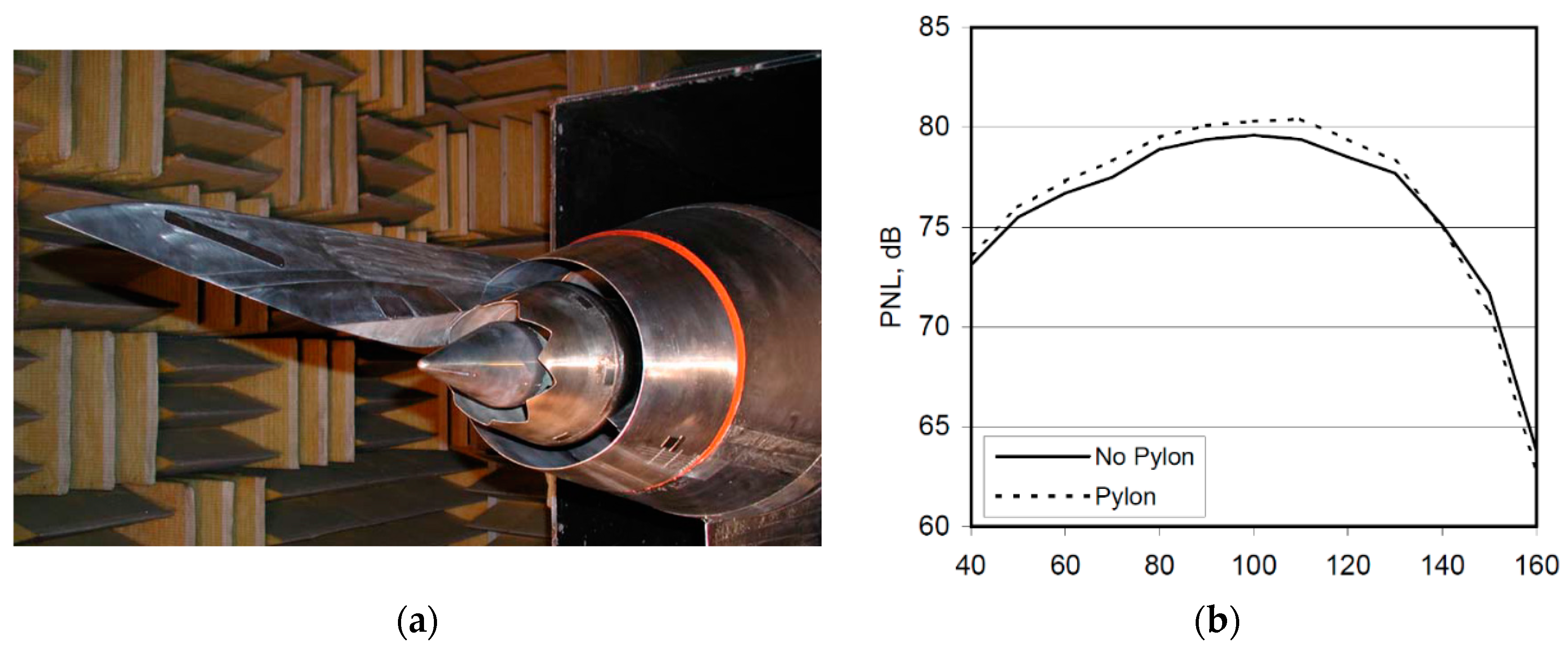
Figure 2.
Illustration of the Coanda and corresponding rooster tail effect.
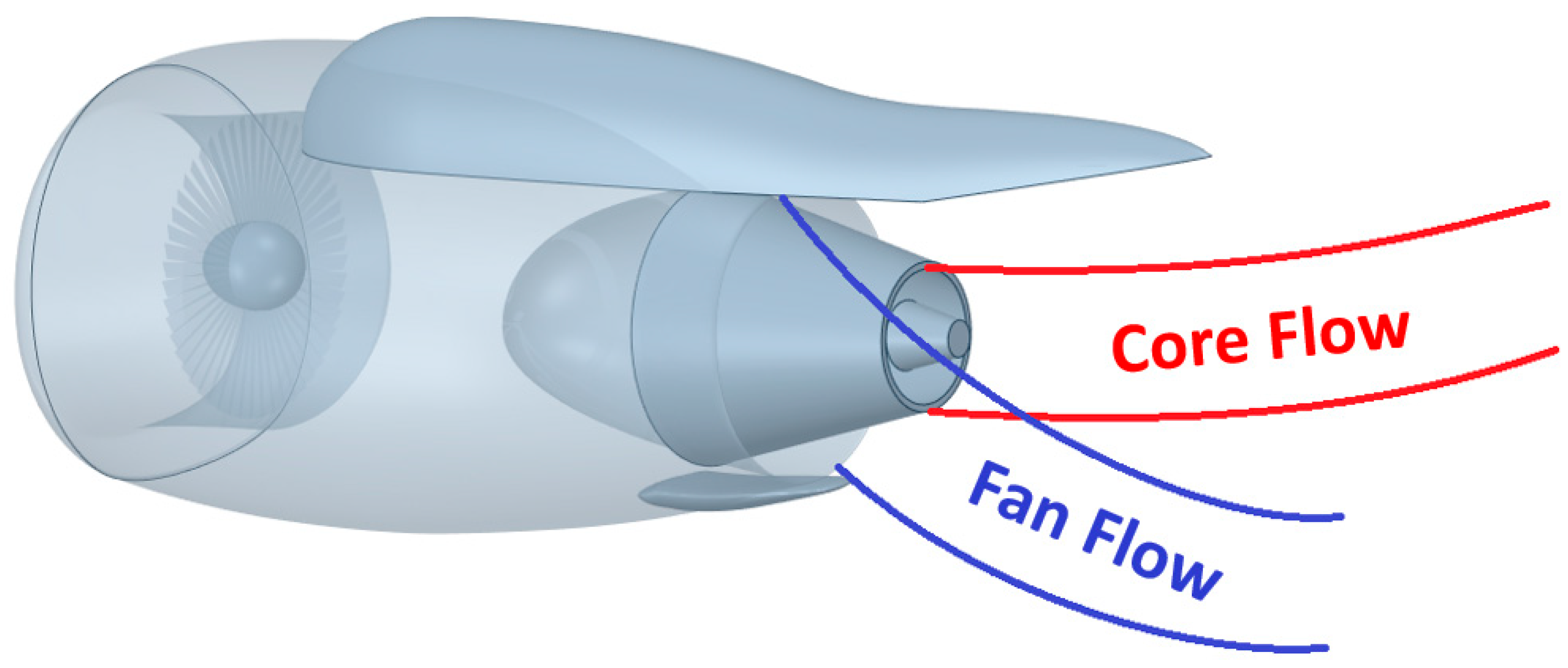
Figure 3.
Schematics of jet flow and acoustic wave interactions with aerodynamic surfaces.

Figure 4.
General Hybrid Wing Body (HWB) configuration (Ref. [24]).
Figure 4.
General Hybrid Wing Body (HWB) configuration (Ref. [24]).
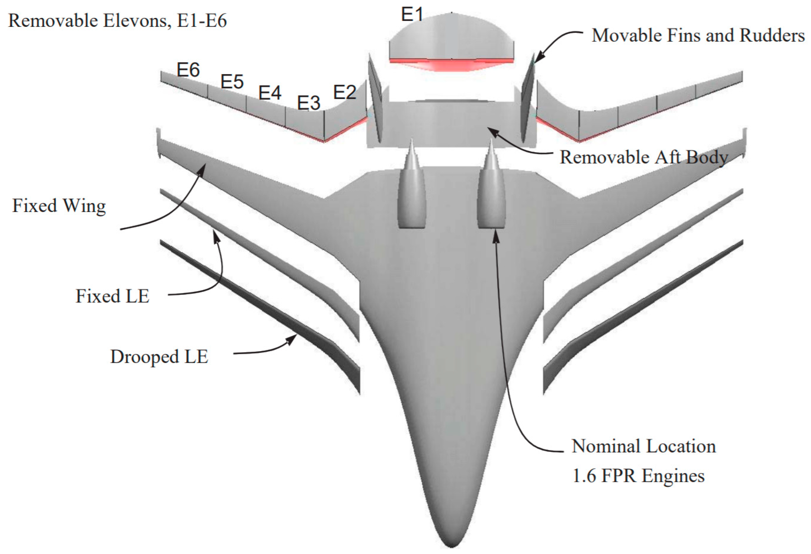
Figure 5.
Jet noise spectral measurements at 90° in a Mach 0.97 rectangular exhaust (Ref [21]).
Figure 5.
Jet noise spectral measurements at 90° in a Mach 0.97 rectangular exhaust (Ref [21]).
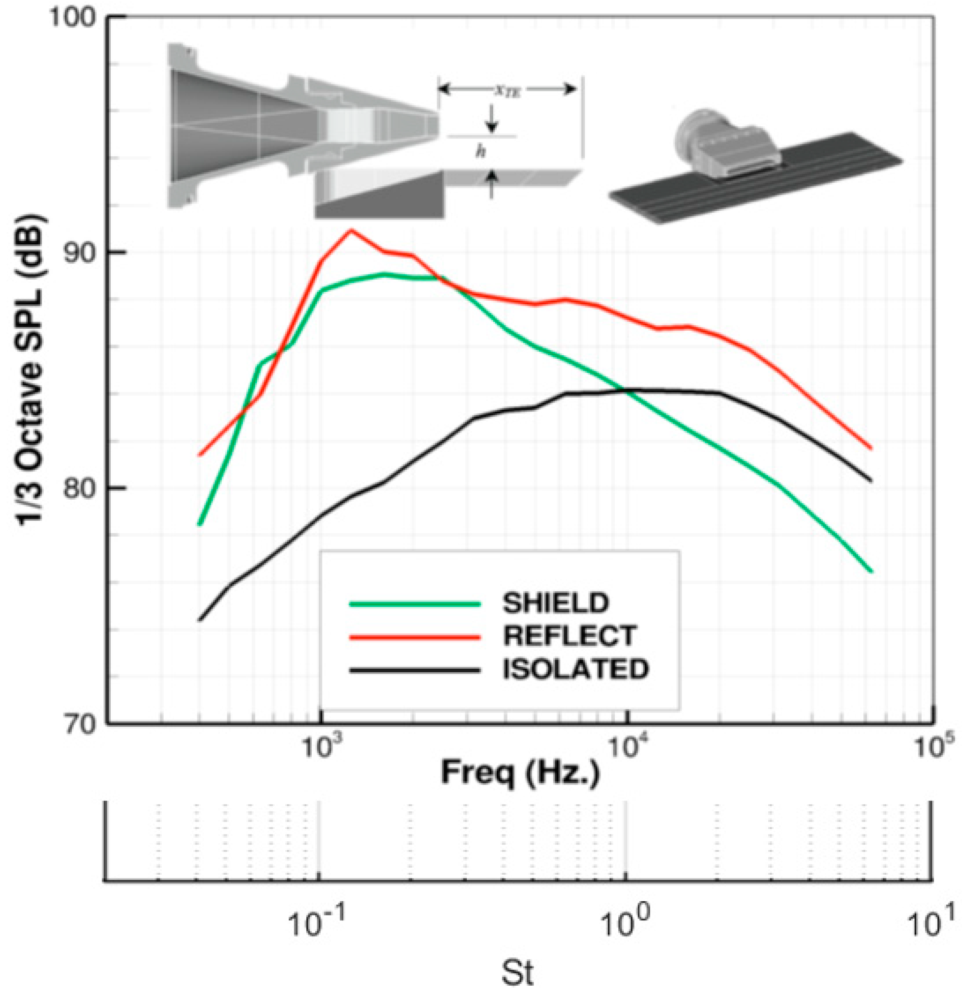
Figure 6.
Jet noise spectral measurements for a supersonic ideally expanded circular jet (Ref. [33]).
Figure 6.
Jet noise spectral measurements for a supersonic ideally expanded circular jet (Ref. [33]).

Figure 7.
Schlieren images of a jet plane (minor-axis plane). (a) Baseline, (b) with plate (). Reproduced from (Ref. [35]), with the permission of the Acoustical Society of America.
Figure 7.
Schlieren images of a jet plane (minor-axis plane). (a) Baseline, (b) with plate (). Reproduced from (Ref. [35]), with the permission of the Acoustical Society of America.
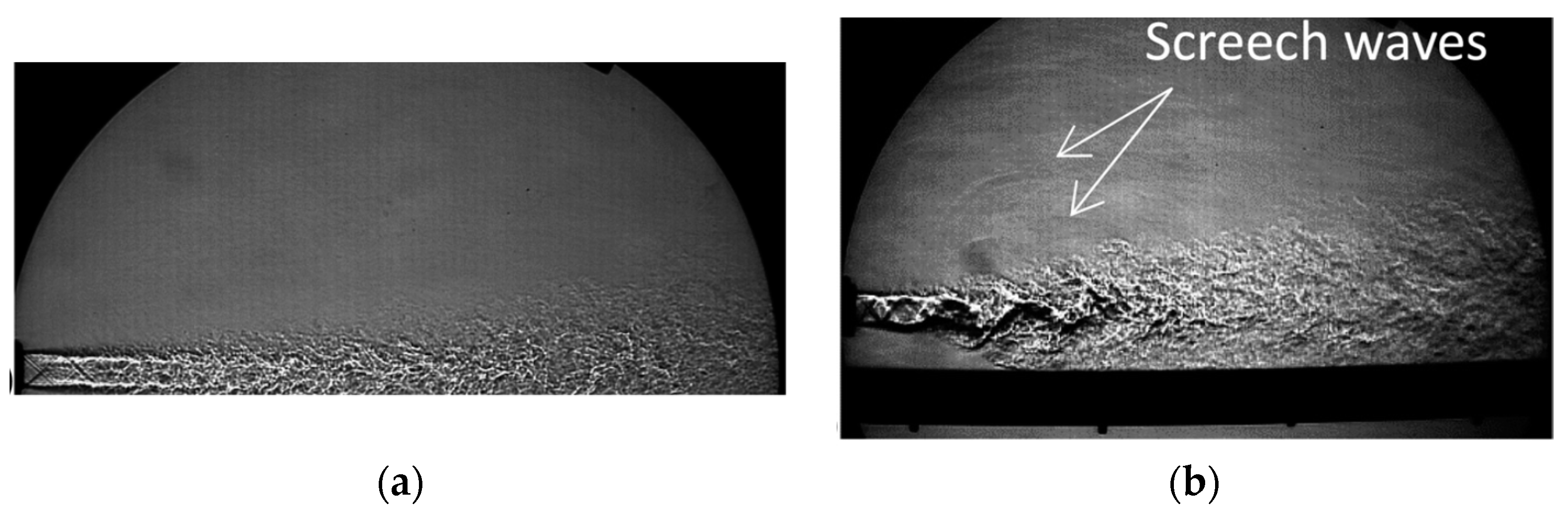
Figure 8.
Far-field acoustic directivity of the (a) reflected side and (b) shielded side. Reproduced from (Ref. [35]), with the permission of the Acoustical Society of America.
Figure 8.
Far-field acoustic directivity of the (a) reflected side and (b) shielded side. Reproduced from (Ref. [35]), with the permission of the Acoustical Society of America.
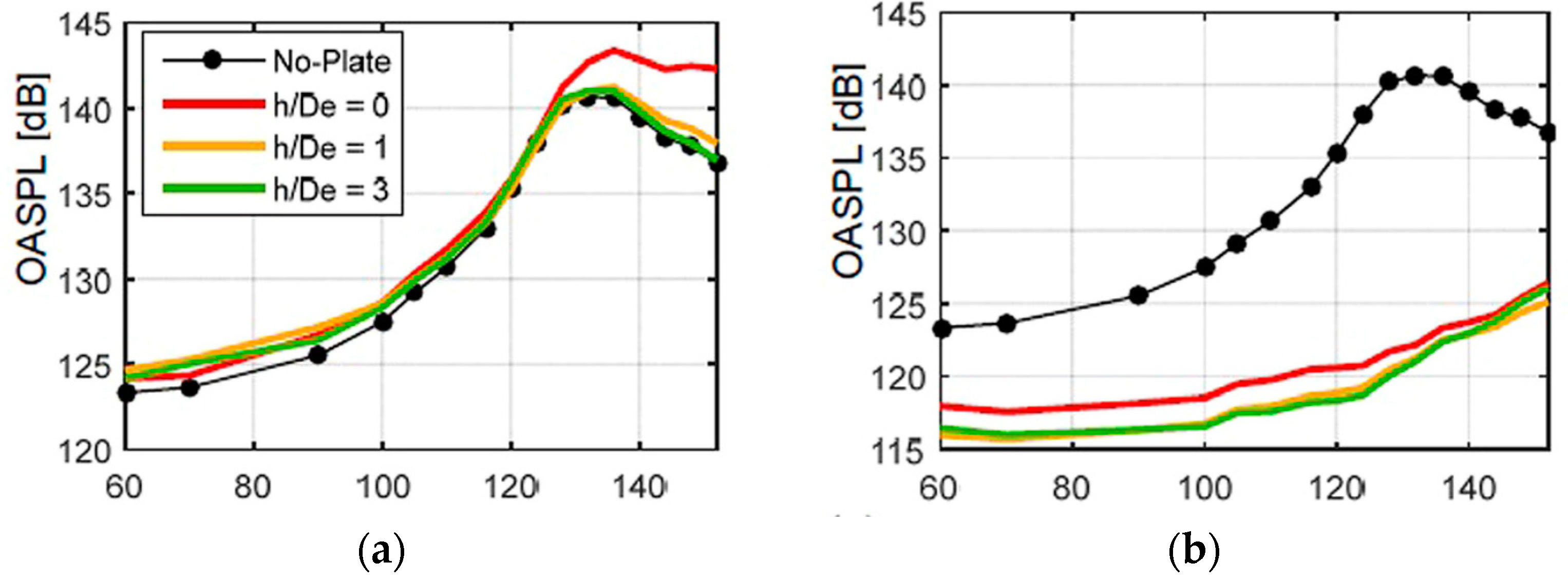
Figure 9.
Peak of the jet noise predicted by Mankbadi and Liu [40] vs. the experimental data of Lush [41].

Figure 10.
Effect of implementing various boundary treatments on the calculated acoustic field associate with an acoustic monopole in a uniform flow (Ref. [49]).
Figure 10.
Effect of implementing various boundary treatments on the calculated acoustic field associate with an acoustic monopole in a uniform flow (Ref. [49]).
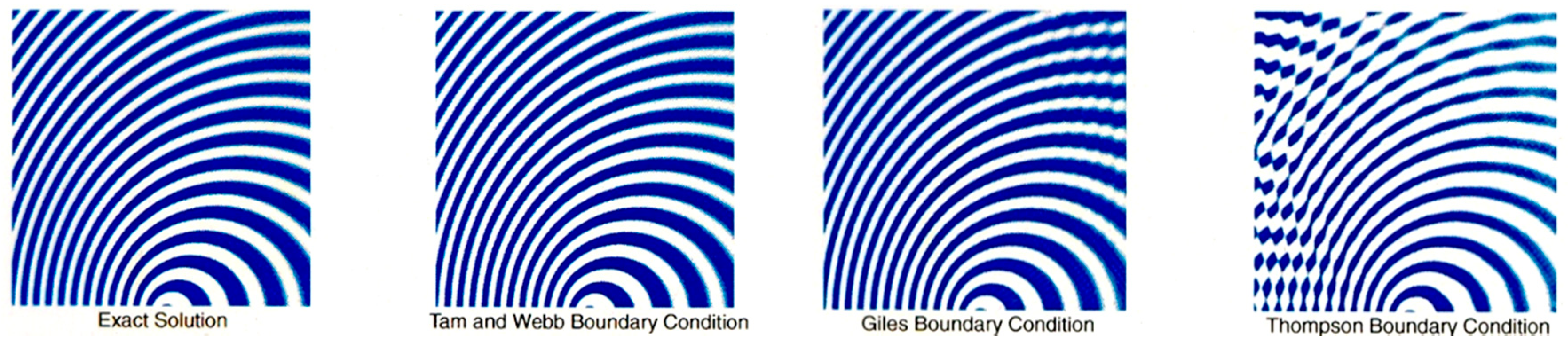
Figure 11.
The radiated acoustic field associated with a point source inside a cylindrical surface calculated using Kirchhoff’s method and with the pressure-only method of Mankbadi et al. [53].
Figure 11.
The radiated acoustic field associated with a point source inside a cylindrical surface calculated using Kirchhoff’s method and with the pressure-only method of Mankbadi et al. [53].
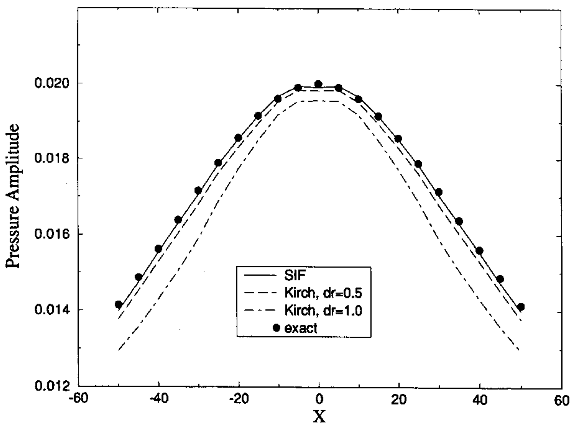

Figure 13.
(a) Directivity of the predicted noise level in dB from the large-scale simulations of supersonic jet noise (Ref. [57]). Compared with (b) the corresponding experimental data (Ref. [59]).
Figure 14.
Full 3D large eddy simulation of a supersonic jet at M = 2.1 excited at the first helical mode showing the pressure near field (Ref. [58]).
Figure 14.
Full 3D large eddy simulation of a supersonic jet at M = 2.1 excited at the first helical mode showing the pressure near field (Ref. [58]).
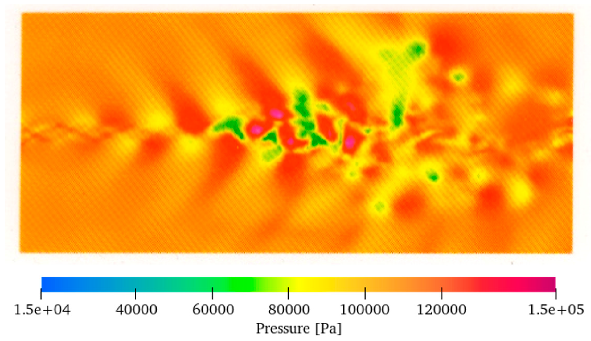
Figure 15.
Prediction of the unsteady flow and acoustics of a supersonic jet using Linearized Euler Equations (Ref. [58,61]). (a) Boundary treatments, (b) Snapshot of the oscillating pressure field, and (c) root mean square of the acoustic pressure distribution.
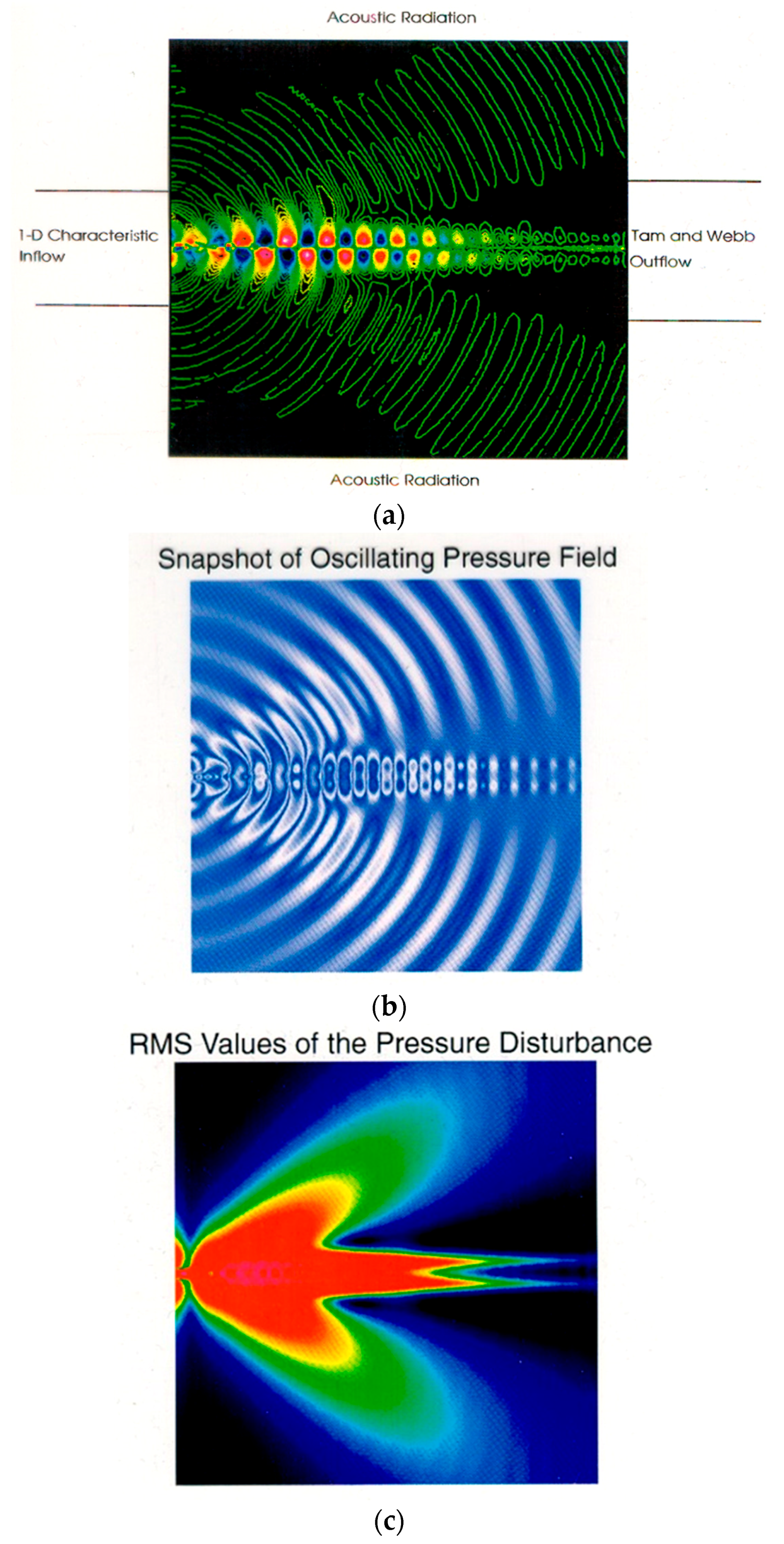
Figure 16.
Prediction of LEE for a supersonic jet M = 21 in comparison with the experiment. (a) Predicted sound pressure level in which the initial disturbances were axisymmetric but was taken either to be at St = 0.2 or computer-generated random disturbances (Ref. [58,61]). (b) Directivity at R/d = 24. The initial input disturbance to jet was taken to be either an axisymmetric or the first helical mode (Ref. [58,59]).
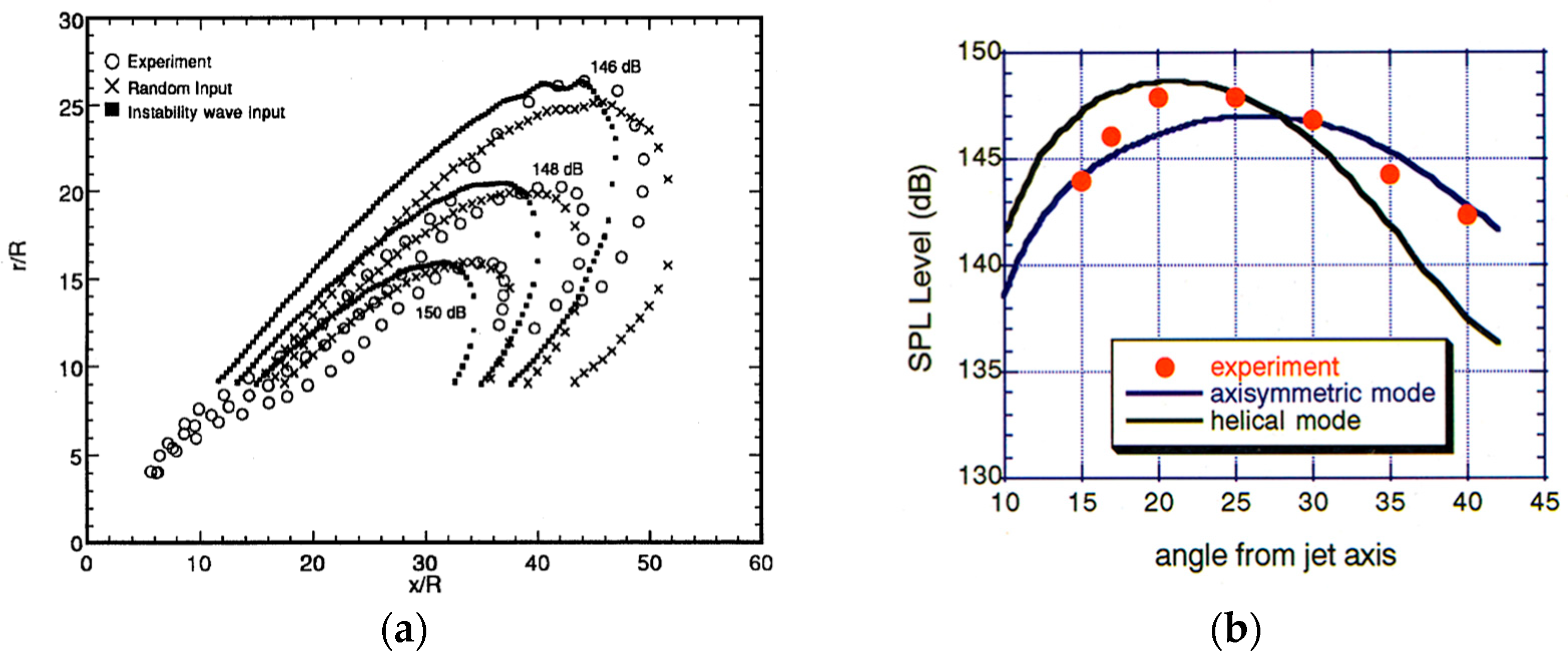

Figure 18.
Very large-eddy simulations. The pressure oscillation at various Strouhal numbers (Ref. [58,62]).
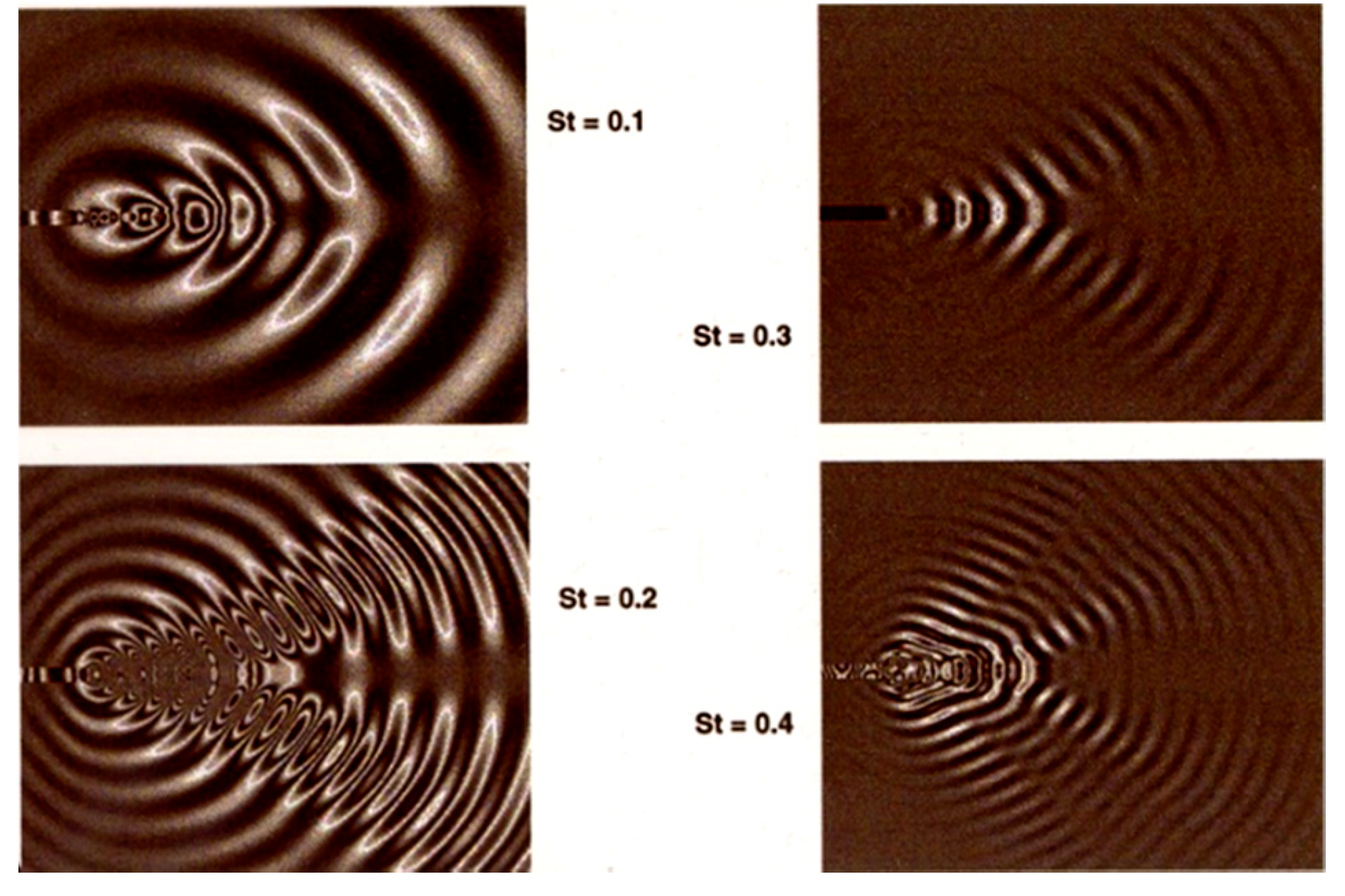
Figure 19.
(a) Development of the momentum thickness for an excitation and unexcited case (a) computation (Ref. [65]) and (b) experimental data (Ref [66]).
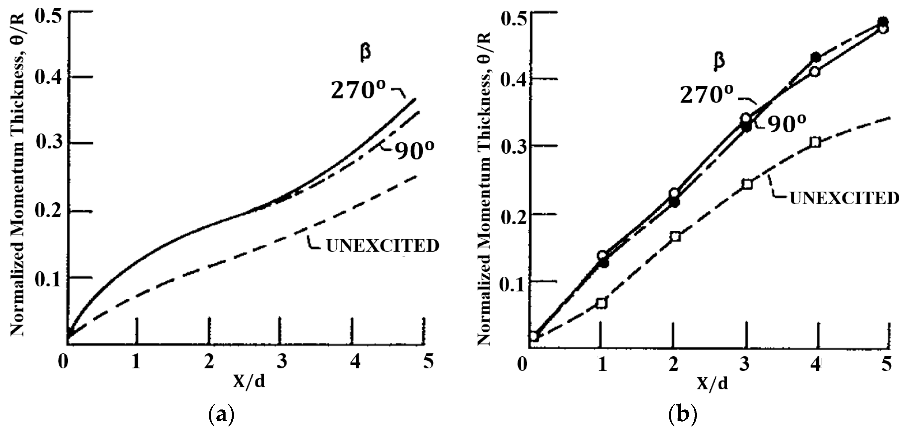
Figure 20.
Snapshots of the instantaneous pressure fluctuations in a round jet for four different cases of inflow excitation with excitation amplitude of . (a) Single frequency . (b) Single frequency . (c) Bi-modal frequency . (d) Random frequency (Ref. [58,71]).

Figure 21.
(a) Nozzle geometry cross-sectional (minor axis plane) and the location of far-field points. (b) Dimension of the flat plate.
Figure 21.
(a) Nozzle geometry cross-sectional (minor axis plane) and the location of far-field points. (b) Dimension of the flat plate.

Figure 22.
Computational grid near the nozzle exit. (a) Baseline case minor plane, (b) Shielded case minor plane, (c) Both baseline and shielded cases major plane.
Figure 22.
Computational grid near the nozzle exit. (a) Baseline case minor plane, (b) Shielded case minor plane, (c) Both baseline and shielded cases major plane.
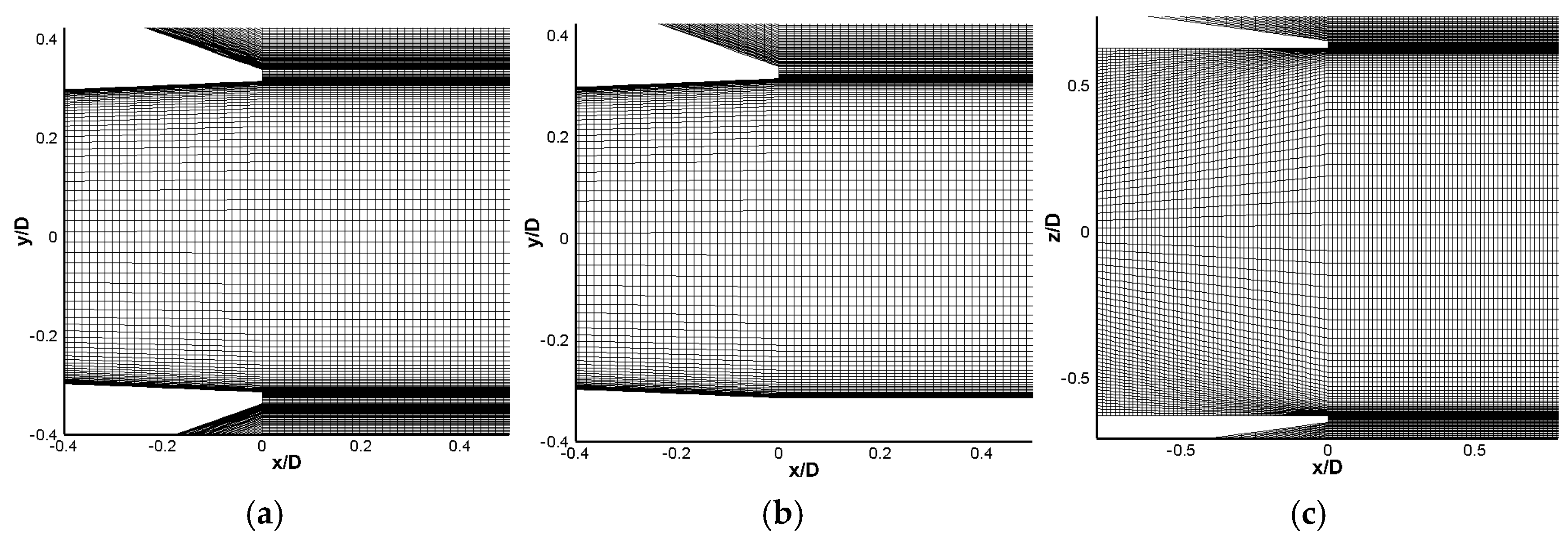
Figure 23.
Computational grid and the refinement regions. (a) Baseline case minor plane, (b) Shielded case minor plane, (c) Both baseline and shielded cases major plane.
Figure 23.
Computational grid and the refinement regions. (a) Baseline case minor plane, (b) Shielded case minor plane, (c) Both baseline and shielded cases major plane.
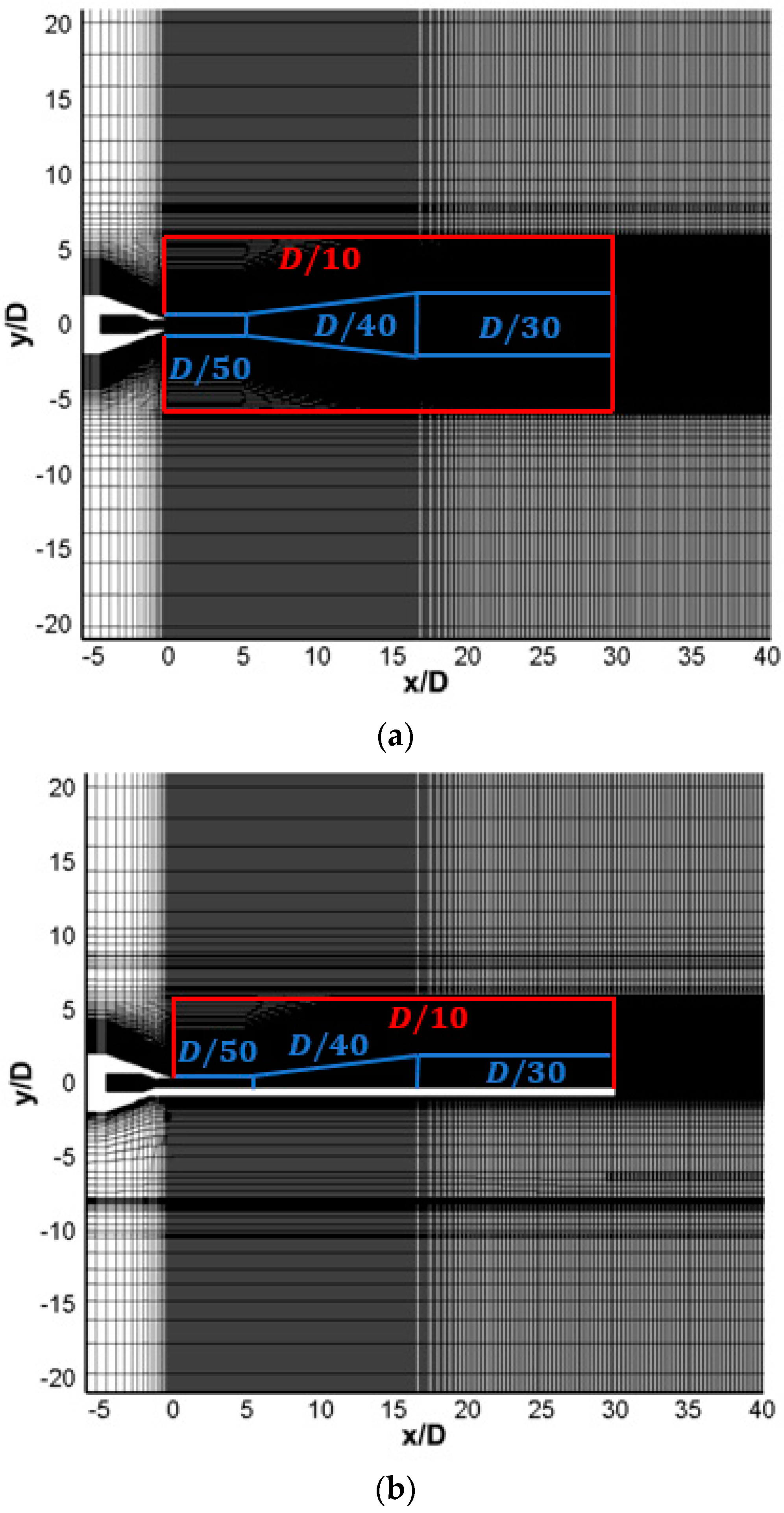

Figure 24.
Time-averaged center line velocity (no plate).
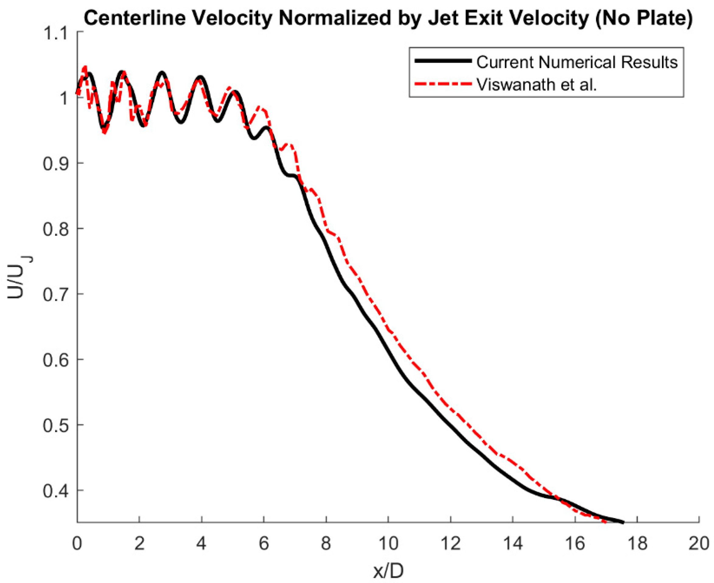
Figure 25.
(a) Instantaneous numerical shadowgraph, (b) Instantaneous Schillerian from experimental measurements (Ref. [35]).
Figure 25.
(a) Instantaneous numerical shadowgraph, (b) Instantaneous Schillerian from experimental measurements (Ref. [35]).
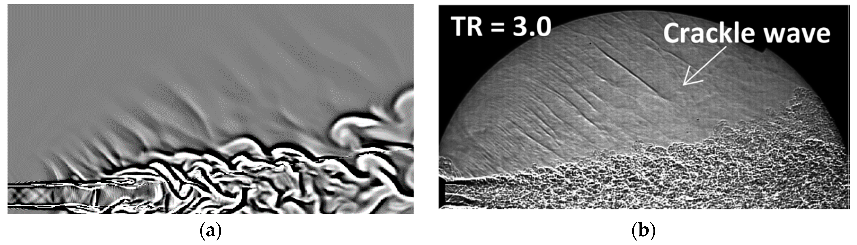
Figure 26.
Time-averaged velocity non-dimensional by jet exit velocity (Shielded case). (a) Numerical (NPR = 3.67, TR = 3.0), (b) Experiment (NPR = 3.67, TR = 2.4) (Ref. [87]).
Figure 26.
Time-averaged velocity non-dimensional by jet exit velocity (Shielded case). (a) Numerical (NPR = 3.67, TR = 3.0), (b) Experiment (NPR = 3.67, TR = 2.4) (Ref. [87]).

Figure 27.
Turbulent kinetic energy normalized by jet velocity squared. (a) Baseline, Numerical (NPR = 3.67, TR = 3.0), (b) Baseline, Experiment (NPR = 3.67, TR = 2.0) (Ref. [88]). (c) With Plate, Numerical (NPR = 3.67, TR = 3.0), (d) With Plate, Experiment (NPR = 3.67, TR = 2.4) (Ref. [87]).
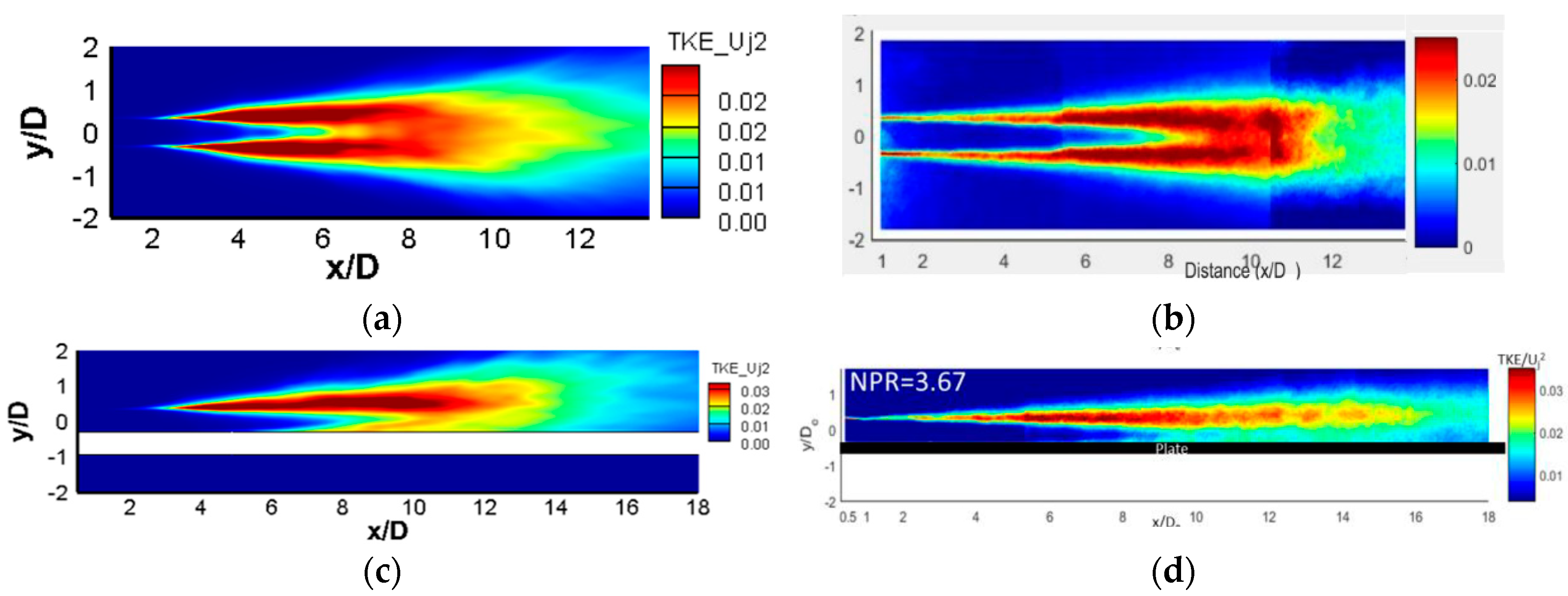
Figure 28.
Instantaneous fluctuating pressure, . (a) Baseline (BSL) case, (b) Shielded case.
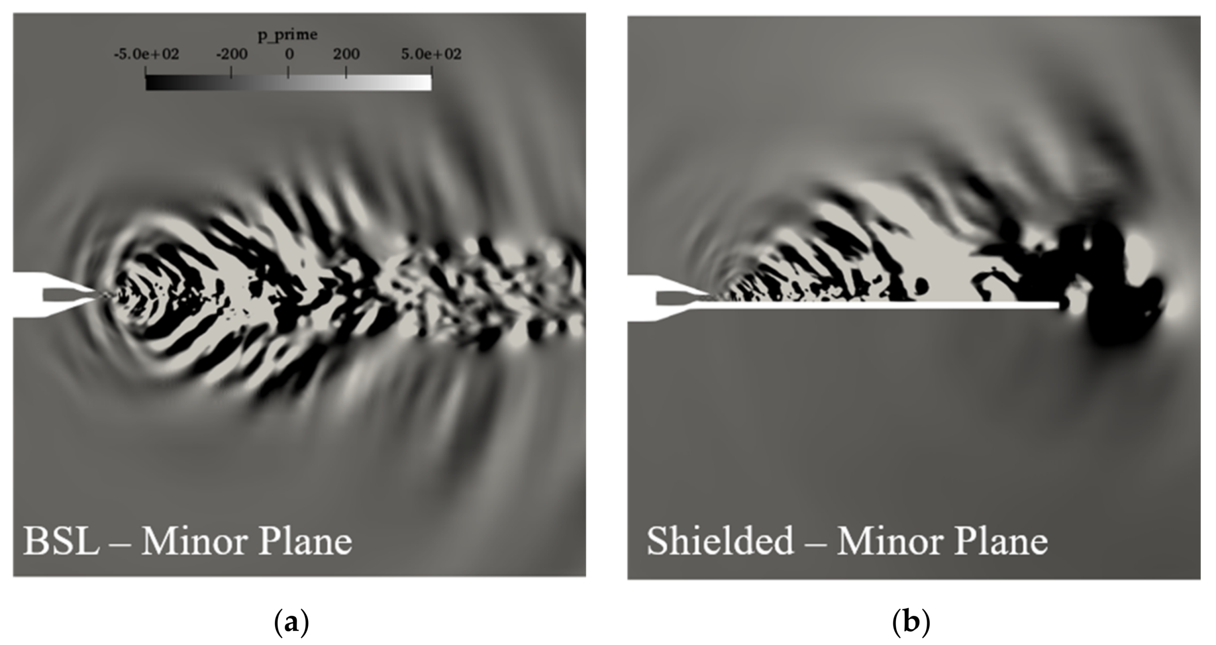
Figure 29.
Acoustic spectra of (a) reflected, and (b) shielded side (no plate).
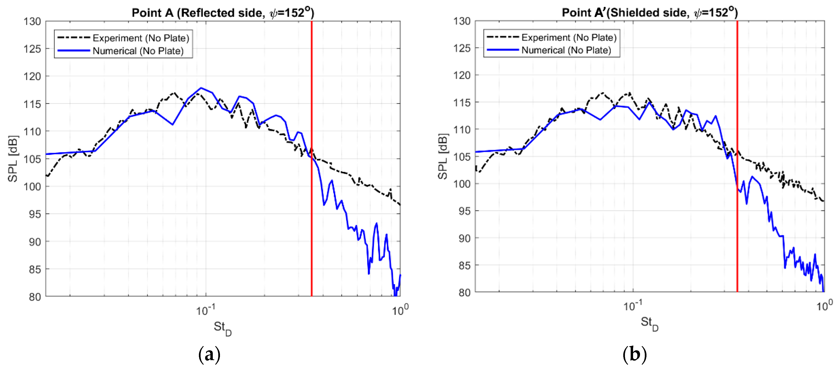
Figure 30.
Acoustic spectra of (a) reflected, and (b) shielded side (with plate).
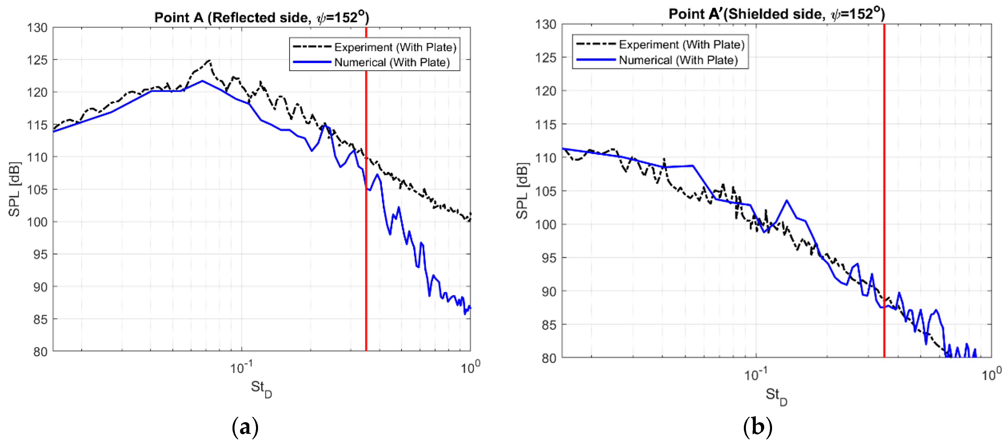
Figure 31.
Evolution of the fluctuating pressure R.M.S along jet axis. (a) Baseline (BSL) case, (b) Shielded case.
Figure 31.
Evolution of the fluctuating pressure R.M.S along jet axis. (a) Baseline (BSL) case, (b) Shielded case.
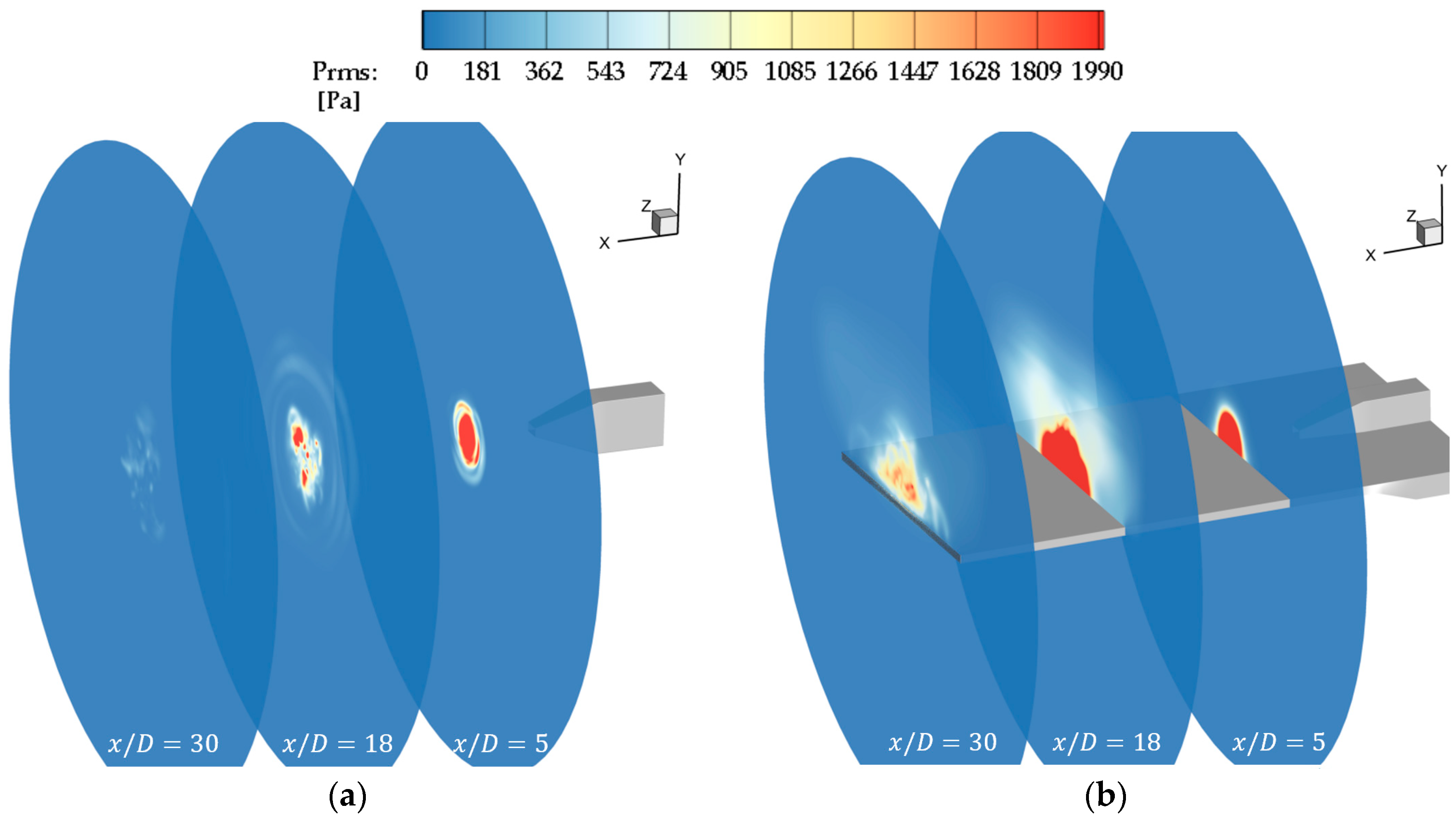
© 2020 by the authors. Licensee MDPI, Basel, Switzerland. This article is an open access article distributed under the terms and conditions of the Creative Commons Attribution (CC BY) license (http://creativecommons.org/licenses/by/4.0/).
Share and Cite
MDPI and ACS Style
Salehian, S.; Mankbadi, R. Jet Noise in Airframe Integration and Shielding. Appl. Sci. 2020, 10, 511. https://doi.org/10.3390/app10020511
AMA Style
Salehian S, Mankbadi R. Jet Noise in Airframe Integration and Shielding. Applied Sciences. 2020; 10(2):511. https://doi.org/10.3390/app10020511
Chicago/Turabian StyleSalehian, Saman, and Reda Mankbadi. 2020. "Jet Noise in Airframe Integration and Shielding" Applied Sciences 10, no. 2: 511. https://doi.org/10.3390/app10020511
Note that from the first issue of 2016, this journal uses article numbers instead of page numbers. See further details here.