2.2. Approximate Method
An analysis of difficult (non-modular) operations has shown that they can be represented exactly or approximately, so the methods for calculating positional characteristics can be divided into two groups:
- –
Methods for accurate calculation of positional characteristics.
- –
Methods for the approximate calculation of positional characteristics.
The methods for accurate calculation of positional characteristics are discussed in [
1,
2,
3]. In this paper, we investigate the approximate method for calculating positional characteristics that can significantly reduce the hardware and time costs due to operations performed on positional codes of reduced capacity. In this regard, there is an issue of using the approximate method when calculating a certain number of non-modular procedures: determining intervals of numbers; number sign; number comparison, in cases where there is no need to know the exact value; and the difference between the numbers.
The point of the approximate method for calculating the positional characteristics of modular number is based on employing the relative values of the analyzed numbers to the full range defined by the CRT, which connects the positional number
a with its representation in the remainder
, where
αi is the smallest non-negative residues of the number in relation to the modules of the residue number system
with the following expression:
where
pi are RNS modules,
is the range of RNS,
, and
is a multiplicative inversion of
Pi modulo
pi.
If we divide the left and right parts of Expression (4) by the constant
P, corresponding to the range of numbers, we will get the approximate value
where
denotes the fraction of
(or Modulo 1 operation) [
24],
are constants of the chosen system, and
αi are positions of the number represented in the RNS in modules
pi, where
, and the value of the Expression (5) will be in the range [0, 1). The result of the sum shall be found after summation and discarding the integer part while maintaining the fractional part of the sum. The fractional value
contains information both on the magnitude of the number and on its sign. If
, then the number
a is positive and
F(
a) is equal to the number of
a, divided by
P. Otherwise,
a is a negative number, and 1 −
F(
a) indicates a relative value. Rounding
F(
a) to 2
−t bits will be denoted as
. The exact value of
F(
a) is determined by inequalities
. The integer part, obtained through summing the constants
ki, is a rank number; that is, a non-positional feature that shows how many times the range of the system
P was surpassed while passing from the number representation in the residue number system to its positional representation. If necessary, the rank can be determined directly through the operation of the summation the constants
ki. The fractional part can also be written as
because
. The number of positions in the fractional part of the number is determined by the maximum potential difference between the adjacent numbers. In case of accurate comparison, which is widely used in the division of numbers, you need to calculate a value that is equivalent to the conversion of the RNS into the positional notation.
Rounding the
F(
a) value will inevitably result in an error. Let us denote
. Work [
22] shows that it is necessary to use
bits after the decimal point when rounding the value
F(
a), so that the resulting error has no effect on the accuracy of calculations. In other words, there is established a one-to-one correspondence between the set of numbers represented in the RNS and the plurality of
values. Using the variables
in calculations, in terms of algorithmic complexity, is equivalent to applying the inverse transformation from the RNS into the positional notation using the CRT. This method is slow and therefore, in practice, the use of calculations with the values
is not rational. In [
22], it is shown that it is possible to use the values
, where
, for operations of determining the number sign in the RNS. The point of this approach is based on the fact that when determining the sign there is no need to know the exact value of the number, and it is just enough to know about the range within which the number tested falls.
The algorithm for determining the sign of the number serves the basis for number comparison algorithms. Determining the sign of the number in the RNS using the values , takes the following operations:
«Rough estimate». At this stage, the value , is used. If , then the number a is positive. If , then the number is negative.
«Clarification». If the number a falls into none of the intervals as indicated in Step 1, then a rechecking of the number is needed with maximum precision calculation regarding the values. If , then the number a is positive. If , then the number a is negative.
The speed of the algorithm at the stage of the «rough estimate» depends on how little the value
is compared to
N. However, if
is taken as too little, then the intervals in Step 1 may be so small that the algorithm for numerous numbers in the RNS would require the use of the «clarification» stage, while the benefit of using a small capacity at the «rough estimate» stage would be dismissed completely. For example, in [
13], it is proposed to use the case when
that is usually too small for practice. Instead, we suggest using an estimation from [
22], which shows that the optimal speed of the algorithm is achieved with
. Here below comes a comparison of the
and
N capacities for the RNS, where the ranges of 16, 32, and 64 bits are implemented.
1. Sixteen bits. RNS modules 7, 17, 19, 29.
2. Thirty-two bits. RNS modules 2, 3, 5, 11, 13, 19, 23, 29, 79.
3. Sixty-four bits. RNS modules 2, 11, 17, 19, 23, 31, 41, 53, 59, 61, 71, 79, 83.
Thus, with an RNS of a 16-bit range, the «rough estimate» is done using the values with a capacity of bits, while the «clarification» takes place at the N = 23 bit precision. The speed of the rough estimate goes up by 2.09 times. For an RNS with a 32-bit range, the «rough estimate» employs a capacity of bits, while the «clarification» requires N = 40 bits for calculation. The speed of the rough estimate increases 3.08 times. For a 64-bit RNS, the «rough estimate» would use a capacity of bits, while the «clarification» requires N = 74 bits. The speed of the rough estimate increases 4.62 times. These results show that, for large ranges, the capacity employed for the rough estimate is significantly lower than the accurate calculation capacity N, which allows significant gains in terms of speed when performing non-modular operations.
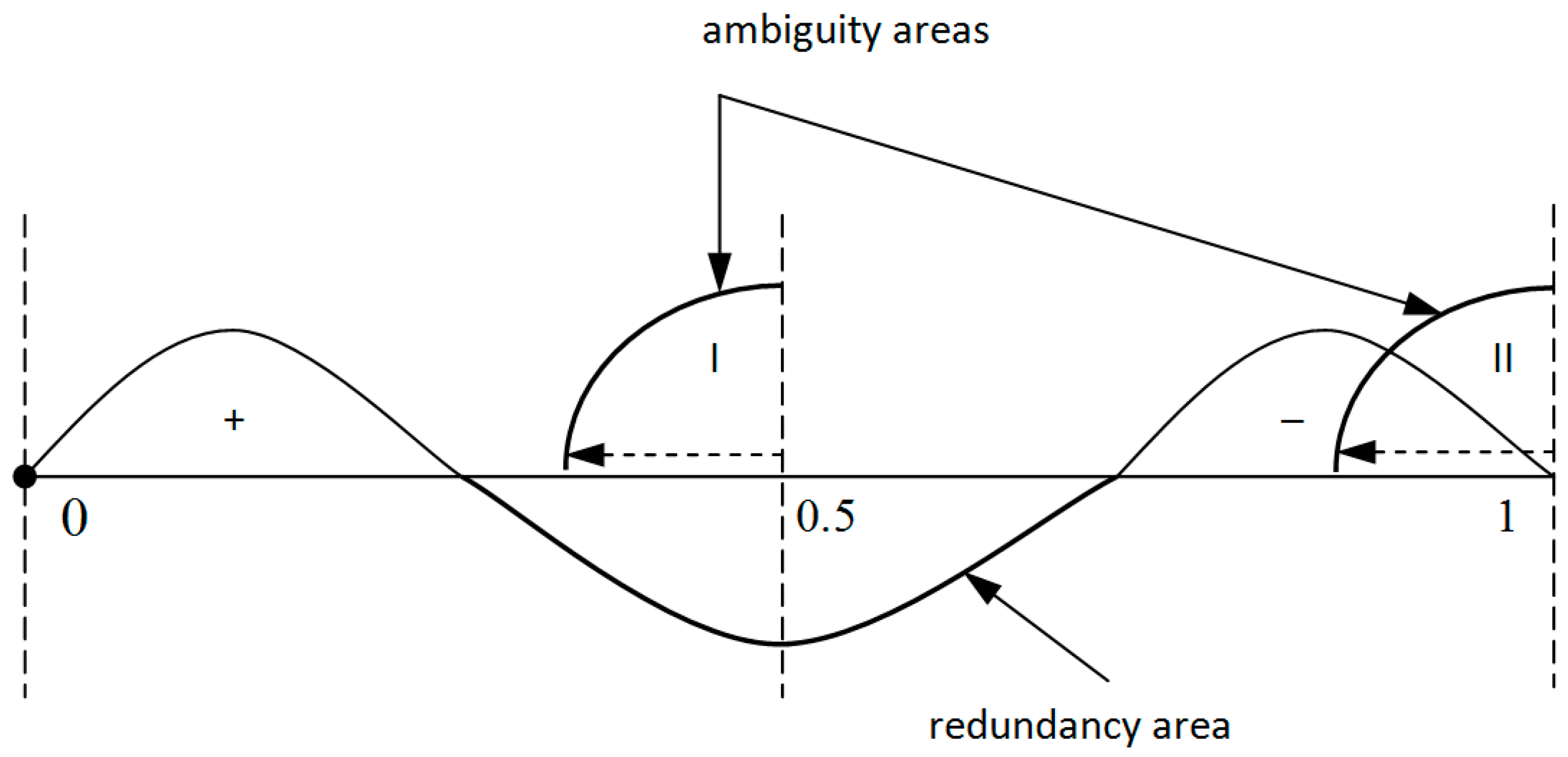
Figure 1 shows the location of the mentioned intervals for positive and negative numbers in the RNS, and the location of the ambiguity areas, where it is possible to wrongly determine the sign. For the redundant RNS, the numerical range shows a redundancy zone. This allows reducing the number of the checked conditions due to the fact that the sets of the admissible positive numbers and the areas of the erroneous sign determination would no longer intersect (
Figure 2). Thus, when speaking of a redundant RNS, determining the sign is reduced to the following tasks.
«Rough estimate». If , then the number a is positive. If , then the number a is negative.
«Clarification». If the number a is not included in any of the intervals in Step 1, then there is a sign rechecking needed using the variables. If , then the number a is positive. If , then the number a is negative.
Let us have a view on employing the approximate method by comparing the numbers in the RNS.
Example 1. We have a system of bases,,,.
Then,,,,,.
The constants
ki used for computing the relative values are:
For precise operations with relative sizes of numbers in the RNS, it is necessary to use characters after the decimal point. For a quick «rough estimate», we will use decimals. The constants ki rounded up to 7 and 12 bits after the decimal point, are, respectively:
Seven bits: k1 = 0.1000000; ; ; ;
Twelve bits: ; ; ; .
The «rough estimate» takes checking the conditions and (Step 1 of the algorithm), which in the binary form will appear as
1.1. If , then the number a is positive.
1.2. If , then the number a is negative.
Let us compare the two numbers a = 97 и b = 8 presented in the RNS on the bases , , , and . Let us define the numbers a and b in the RNS as: a = (1, 1, 2, 6), b = (0, 2, 3, 1). The difference is a − b = (1, 1, 2, 6) − (0, 2, 3, 1) = (1, 2, 4, 5). We will also define the sign a − b. For the «rough estimate», we will find that . The values found meets the condition of Step 1 of the algorithm, that is 0 < 0.0110001 < 0.0110011, so we can conclude that a – b > 0, which produces a > b.
Now, let us compare the two numbers a = 97 and b = 96 as presented in the RNS on the bases , , , and . Now, we will define the numbers a and b in the RNS: a = (1, 1, 2, 6), b = (0, 0, 1, 5). The difference is a − b = (1, 1, 2, 6) – (0, 0, 1, 5) = (1, 1, 1, 1). We will define the sign a − b. For the «rough estimate», . None of the conditions are met regarding the value obtained, so it will take a clarification stage of the algorithm. For the «accurate estimation», we will find . This value follows the condition of Step 2 of the algorithm, so we conclude that a – b > 0, where a > b.
The example above serves an illustration of employing the approximate method for computing in the RNS. It has been shown how to take into account the error that occurs when using a small . In practice, for most cases, it would be enough to carry out a «rough estimate», a run wherein it takes operating with numbers whose capacity is close to the logarithm of the full range capacity. Therefore, the complexity of the «rough estimate» is committed to , while the complexity of the «clarification» stage tends to O(n).
2.3. Division Algorithm in the RNS
The algorithm for the integer division could be described with an iterative scheme, which is performed in two stages. The first stage implies a search for the highest power 2i when approximating the quotient with a binary sequence. The second stage involves clarification of the approximating series. To get a range greater than P, you can select a value ; thus, it will take expanding the RNS base through adding an extra module. To avoid this base expansion, which is a computationally complex operation, we need to compare not the dividend with the interim divisors but the current results of the iteration (i) with the values of the previous iterations (i − 1). We will repeat the process of doubling the divider as long as the intermediate divider at the i iteration is below that of the i − 1 iteration. This would allow meeting the condition .
The division algorithm can be described with the following rules.
A certain rule φ is constructed, which, for each pair of positive integers, a and b will assign a certain positive number qi, where i is the number of the iteration, so that , i.e., . Then, the division of a by b will follow the rule: based on the operation φ, each pair of a and b will be assigned a corresponding number , so that , i.e., . We will take the values 2i as and place them into the memory as the constants . Given that, the i + 1 operation does not depend on the i-th operation, which allows performing iterations in parallel. Furthermore, in each iteration, there are only two operations performed: multiplication of the constant divisor by 2i, and comparison of the obtained values with the dividend.
If
, then the division is complete; if
, then following the rule
φ, the pair of numbers
will get a
q2 assigned, so that
, i.e.,
. If
, then the division is completed, and if
, then following the rule
φ, the pair of numbers
is assigned a
q3, so that
, etc. Since the consistent application of the operation
φ leads to a decreasing sequence of integers
, then the algorithm is implemented in a finite number of steps. Let us assume that at step
m there is a case 0 <
bqm recorded, which means the end of the division operation. Then, we finally obtain
, where the sequence
is the approximation of the quotient, which may contain some extra
qi. Next, we need clarification for the resulting approximating series. In [
14] and [
16], the idea of the most significant bits for the quotient was introduced for RNS with specialized moduli sets
and {2
k, 2
k − 1, 2
k – 1− 1}, while the approach proposed in this paper is extended for a general case.
The clarification will start with the higher
qm. If
a >
bqm, then
qm is a member of the approximating series of the resulting quotient. Further, we take
: if
, then
is put into the line, otherwise, if
, then
qm is excluded from the series, etc. After checking all the
qi, the quotient shall be determined by the remaining members of the series. Then, the quotient desired is determined by the expression
, where
This algorithm will be easy to modify it into a modular form, while the absolute values of the variables are replaced with their relative values. The structure of the algorithm proposed is based on employing the approximate method for comparing numbers, which is performed using subtraction.
The known algorithms determine the quotient on the basis of iteration , where A and , respectively, are the current and the next dividend, D is the divisor, Q1 is the quotient, which is generated at each iteration of the full range of the RNS, and is not chosen from a small set of constants. In the proposed algorithm, the quotient is determined from the iteration , where A is a certain dividend, b—divisor, and 2i is a member of the quotient’s approximating series.
A comparison of the algorithms shows that the dividend in all iterations does not change, while the divisor is multiplied by the constant, which significantly reduces the computational complexity. In the iterative process of division in positional notation, in order to search for the highest power of the quotient’s approximating series, and to clarify the approximating series, the dividend is compared to the doubled divisors or to the sum of the members of the series. Application of this principle to RNS can lead to incorrect operation of the algorithm, since, in case of the dynamic range overflow for the intermediate divider, the reconstructed number may go beyond the operating range caused by cyclic RNS. The cyclic RNS value will be below the dividend, which is not true because, in fact, the numbers will exceed the range P and the algorithm will proceed to the «loop» mode. For example, if the RNS modules are , , , and , then the range is . Suppose the reconstruction produced the number A = 220. In the RNS, , i.e., A = 210 and have the same representation in the RNS. This ambiguity can lead to a breach of the algorithm. To overcome this difficulty, there is a need to compare the RNS the results of the current iteration values with the previous ones, which allows correct determination of a larger or smaller number. So, the fact of the dynamic range overflow in the RNS can be used for decision-making, «more-less». At the first iteration, there is a comparison of the dividend with the divisor, while the remaining iterations compare the doubled values of the divisors . Each new iteration implies a comparison of the current value with the previous one.
Consistent application of these iterations leads to the formation of the inequalities chain , which determines the required number of iterations dependent on the values of the dividend and the divisor. Thus, the algorithm is implemented through a finite number of iterations. Suppose that at iteration there is a case of closure of the increasing sequence , which corresponds to the RNS overflow range, i.e., and . Here is the end of the process of developing quotient interpolation through a binary sequence or a set of constants in the RNS. Thus, the process of the quotient approximation can be done by comparing the neighboring approximate divisors.
Here below, we will provide a detailed description of an improved algorithm for the division of modular numbers in a redundant RNS.
2.5. Clarification of the Quotient’s Approximating Sequence
Step 5. From the memory, we select the constant 2j (the highest power of the series) and multiply it by the divisor. The value 2jF(b) will be compared with the dividend F(a) using the approximate method of number comparison in the RNS.
The constants 2j, are previously placed in the memory V; the counter j and the quotient Q are set on «0». The outputs of the counter are address inputs in the memory V.
Step 6. Calculate the . If the sign bit the value is «1», then the corresponding power series is discarded; if the value is «0», then to the quotient adder we add the value of the sequence members with the same degree, i.e., , , .
Step 7. Check the sequence member of the degree through a shift to the right and comparison. Compare and . If , then the corresponding power series is discarded; if , then to the quotient adder we add the value of the sequence members with the same degree, i.e., и .
Step 8. Similarly, check all the remaining sequence members up to degree zero. The last , i.e., 0 ≤ R < b will be the remainder of a divided by b. The quotient Q will be the sum of all the 2j needed for developing the quotient, which was accumulated in the adder with the sign as defined in the second step. The algorithm terminates.
The performance of the modified algorithm could be further shown with the example below.
Example 2. Find the quotientof dividingbyin an RNS with bases,,,. Then,,,,, and.
The constants
ki used for calculation of the relative values are:
For a quick «rough estimate», we will use characters after the decimal point. The constants ki rounded up to 7 bits after the decimal point are:
Seven bits: ; ; ; .
Precise operations with relative values of the numbers in the RNS take
characters after the decimal point. The constants
ki rounded up to 12 binary bits after the decimal point are:
Now, we shall represent the
a и
b numbers in the RNS:
Determine the signs of the numbers a and b.
A «rough estimate» (binary):
Since
misses any one of the intervals
,
as set forth in Example 1 will take a clarifying iteration:
, too, misses all the intervals , as set forth in Example 1, so it will take another clarifying iteration.
Since
, then the number
is positive.
Since , then the number b is negative.
The numbers a and have opposite signs, so the quotient sign will be negative. In order to find the absolute value of the quotient, we will divide a by following the algorithm as specified above.
The relative values of the dividend
a and the divisor −
b with full accuracy of the calculations
are:
Shifting the fractional part of the divisor −
b to the left, step by step, we determine that a change in the first fractional bit after the decimal point occurs at the fourth shift. Thus, the approximation series can include only the values 2
0, 2
1, 2
2, and 2
3, which, in the RNS, have the following representation:
These values develop the approximation sequence of the quotient, which is to be clarified later on. For a more accurate approximation sequence, we will subtract from the fraction
of the dividend the fraction of the divisor
that has been shifted three ranks to the left (i.e., multiplied by 2
3):
Since , then we will leave 23 in the approximation sequence, while the value will be used for further calculations.
We subtract from
the fraction
of the divisor shifted left two ranks:
Since , then we leave 22 in the approximation sequence, while the value will be used for further calculations.
We subtract from
the fraction
of the divisor shifted left one rank:
The appearance of 1 in the sign rank indicates that , therefore 21 is excluded from the approximation sequence, and is not to be used further (continue using ).
We subtract from
the fraction
of the divisor (no shift applied):
The appearance of 1 in the sign rank indicates that , so 20 is excluded from the approximation sequence.
Here, the process of clarifying the approximation sequence comes to an end. To determine the quotient, we need to add the remaining members of the approximation sequence. In this example, the remaining members were the following ones:
and
. Then the absolute value of the quotient is to be determined through summing the members of the sequence:
In view of the sign, we finally obtain .
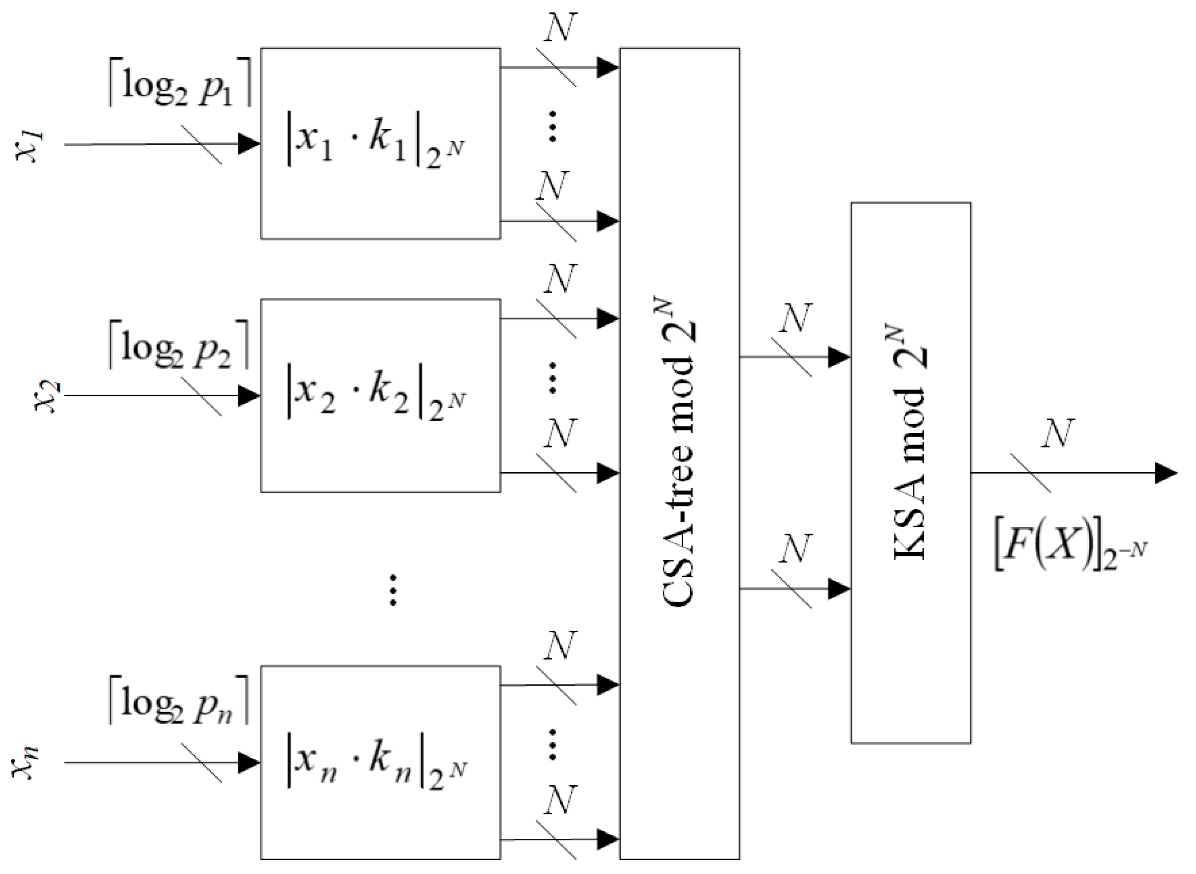
Figure 3 demonstrates the scheme of positional characteristics calculation based on CRTf for a number
. A bit’s width of values
xi is equal to
,
. The initial moduli
,
generates partial products of constant multiplication. Then, they are summed by a Carry-Save-Adder-tree (CSA-tree) modulo 2
N. Obtained results are summed by Kogge–Stone adder [
25] modulo 2
N and is equal to
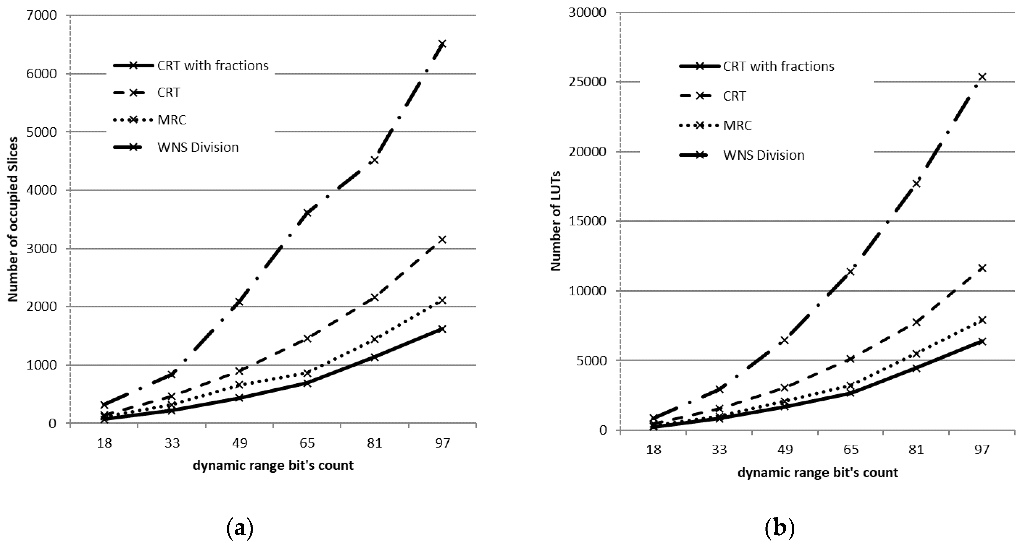
. In the next section, we will demonstrate the advantages of the proposed method compared to known analogs based on CRT and MRC.


 ,
, 


