Effect of High-Temperature Pavement Paving on Fatigue Durability of Bearing-Supported Steel Decks

Abstract

Orthotropic steel deck (OSD) is a better choice for urban bridges and the replacement of damaged concrete slabs. Gussasphalt concrete (GAC) is usually adopted as the asphalt surfacing; however, the paving temperature of GAC is high, which will affect the fatigue durability of fatigable welds in OSD. In this study, such influence of high-temperature pavement paving was comprehensively investigated based on in-situ monitoring and numerical analysis. The temperature of OSD and displacement of bearings were investigated based on the monitored data and numerical results. After that, the deformation and residual temperature stress of OSD during the paving process were analyzed. On this basis, the effect of residual temperature stress on fatigue damage accumulation of OSD was investigated and discussed. Results show that the uplift and expanded deformation of OSD arise during the paving process, leading to the displacement of bearings. Residual displacement of bearings, as well as the residual temperature stress at fatigable details of OSD, is observed. The residual temperature stress has considerable effect on fatigue damage accumulation at rib-deck weld. A fatigue damage amplification factor of 1.1 is recommended for taking into consideration of the adverse effect of high-temperature pavement paving.

1. Introduction

Orthotropic steel deck (OSD) has been widely used in long- and medium-span bridges because of their light weight, high strength, and other advantages [1]. Moreover, OSD gradually becomes a better choice for the replacement of concrete slabs of old concrete bridges. For example, Nanjing Yangtze River Bridge replaced its concrete slab by OSD in the year of 2018, which will be introduced in detail in the next section. For these reconstructed bridges, the OSD is usually placed on the main beams using a set of bearings. During the process of high-temperature pavement paving, OSD will surfer obvious deformation, as confirmed in [2]. Large deformation of OSD will affect the service performance of bearings (i.e., resulting in residual displacement). The residual displacement of bearings will in turn restrict the deformation recovery of OSD, generating residual stress at fatigable details (i.e., residual temperature stress). Due to the coupled effect of vehicle-induced stress, welding residual stress, and residual temperature stress, the fatigable details will be more prone to fatigue cracking. Therefore, it is necessary to reveal the effect of high-temperature pavement paving on fatigable details for precise fatigue damage evaluation.

Actually, based on the principle of superimposed stresses, the effect of residual temperature stress could be equivalent to that of stress ratio (R), as illustrated in Figure 1. After taking into consideration the welding residual stress, both R and the mean stress (σ_m) has increased. Furthermore, both R and σ_m have further increased due to the effect of residual temperature stress. The increase of R and σ_m will subsequently affect the fatigue performance of fatigable welds, as evidenced by extensive experimental and numerical studies, which show that the fatigue strength of welds decreases when the stress ratio (or mean stress) increases [3,4,5]. On this basis, the fatigue damage might be underestimated when neglecting the effect of high-temperature pavement paving. Therefore, it is necessary to clarify and quantify such effect on fatigable welds in OSD.

For this purpose, in-situ monitoring is one of the most effective methods [6]; however, it is impractical to install enough sensors or strain gauges. Furthermore, the monitored data are usually insufficient to predict the distribution and variation of temperature and thermal stress. Instead, the finite element (FE) method is commonly adopted to investigate the thermal characteristics of OSD [7,8]. To make the FE model more accurate and reliable, monitored data are usually used to verify the feasibility of the model. Hence, a numerical analysis combined with in-situ monitoring is often adopted for thermal analysis [2,9]. Recently, most studies have been focused on the thermal field induced by ambient temperature, solar radiation, wind, humidity, and their combined effects [10,11,12], while a few studies have assessed the effects of high-temperature pavement paving on the fatigue performance of OSD. The effect of high-temperature pavement paving on the thermal field characteristics and thermal deformation of OSDs of Tongling Yangtze River Bridge and Taizhou Yangtze River Bridge were investigated, of which the OSDs are supported by cables [2,9]. The analytical methods are referable; however, the effect of high-temperature pavement paving on the fatigue performance of OSD is not mentioned. Hence, further studies are needed, especially for the OSDs supported by bearings.

Overall, the objectives of this study consist of (1) investigating the thermal characteristics of bearings-supported OSD during high-temperature pavement paving; (2) investigating the variation of residual temperature stress during the paving process; (3) evaluating the effect of residual temperature stress on fatigue performance of OSD during its service life. To accomplish the objectives, both in-situ monitoring and FE analysis were carried out. Firstly, the thermal characteristics of OSD were analyzed based on in-situ monitoring results. After that, the transient thermal analysis-based finite element model was established and verified based on the monitored data. Subsequently, the deformation of OSD and the variation of residual temperature stress were analyzed. Finally, the effect of residual temperature stress on fatigue performance of OSD was evaluated based on a proposed evaluating framework. The research flow chart is shown in Figure 2. The results address the significance of residual temperature stress in fatigue damage evaluation, especially when a precise evaluation result is needed.

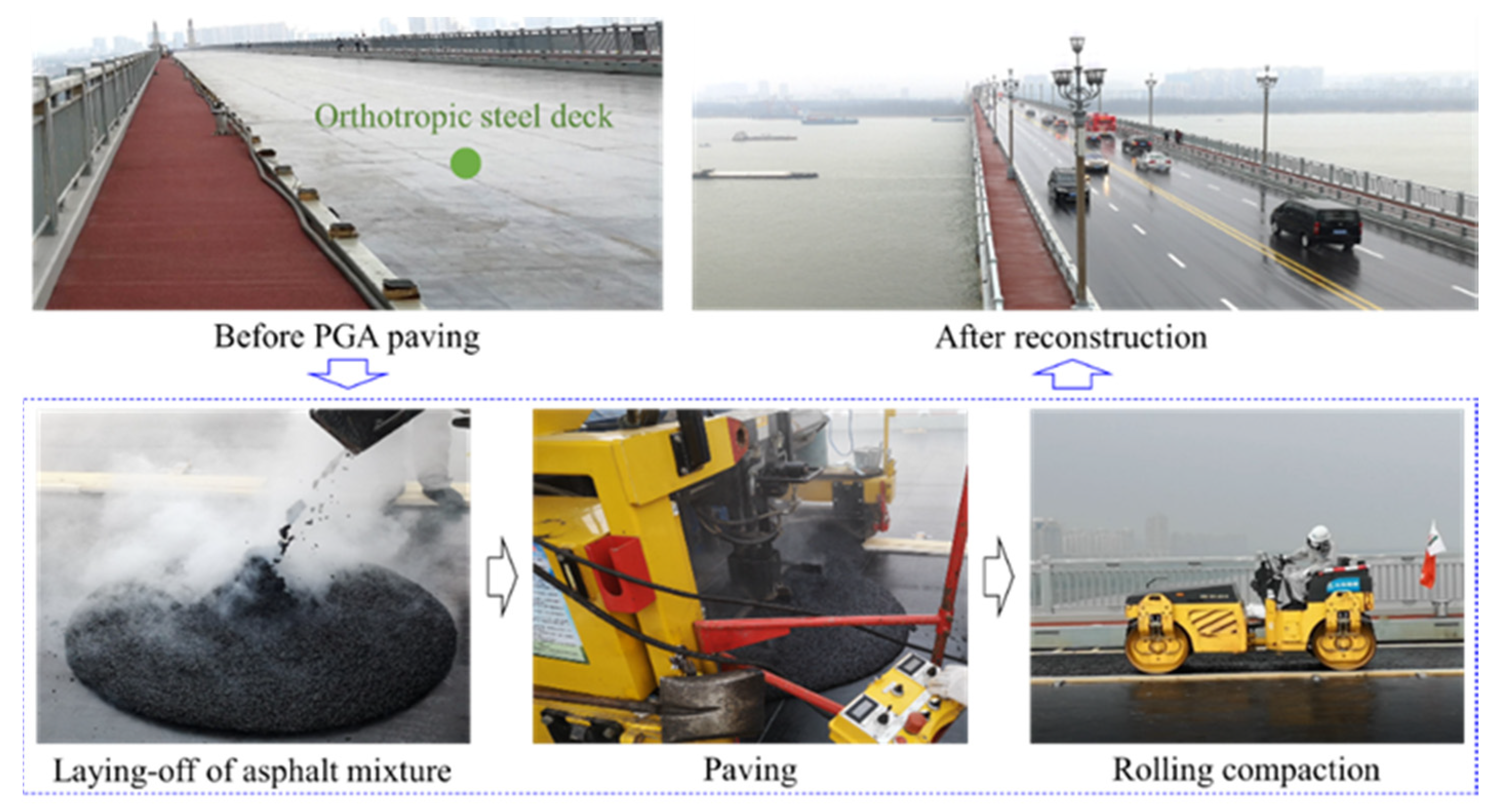
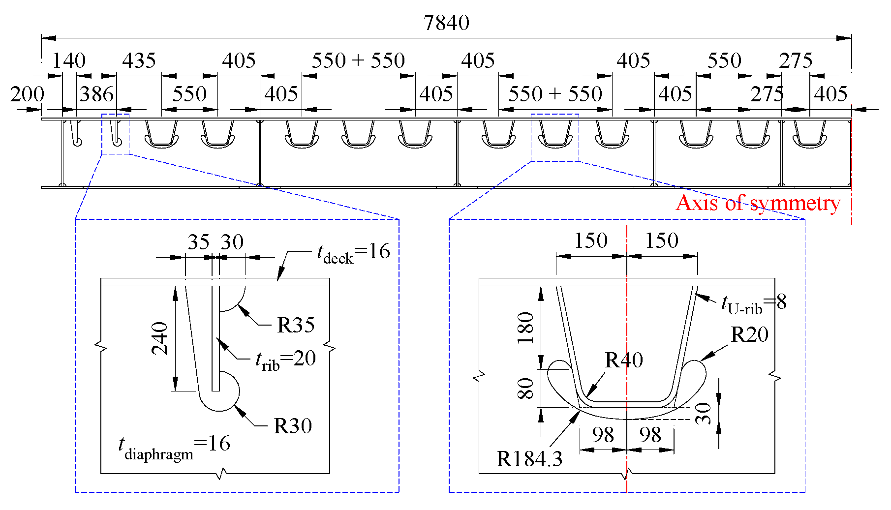
2. Background of Project

The Nanjing Yangtze River Bridge (NYRB) was selected as the object of this study. The NYRB, opened to traffic in 1968, was the first bridge to cross the Yangtze River in China. Additionally, it was the first self-designed double-deck railway and highway bridge in China. The NYRB was recorded as “the world’s longest bridge with dual functions of railway and highway” by the Guinness Book of World Records in the 1960s. The NYRB is not only the important pathway crossing rivers in eastern China, but also one of the transportation junctions serving Nanjing City. After nearly 50 years of service, the railway maintains good working performance, however, the highway composed of concrete deck slabs has faced a series of defects (e.g., pothole and rutting of pavement, serious corrosion of expansion joint, cracking of the concrete slab). To improve the service properties of the NYRB, the concrete deck slabs have been replaced by orthotropic steel deck (OSD) (Figure 3).

The reconstruction project began in October 2016 and was completed in December 2018. The railway kept in service during the whole reconstruction process. The OSD was placed above the main beams using a set of tension-compression bearings. After that, pouring Gaussian asphalt (PGA) concrete, a widely used pavement material for OSD, was adopted in the pavement paving process (see Figure 3). Generally, PGA has the highest temperature (reaching 220–260 °C) among all paving materials. As introduced in Section 1, it might affect the fatigue performance of OSD, which is mainly focused on in this study.

3. Field Monitoring

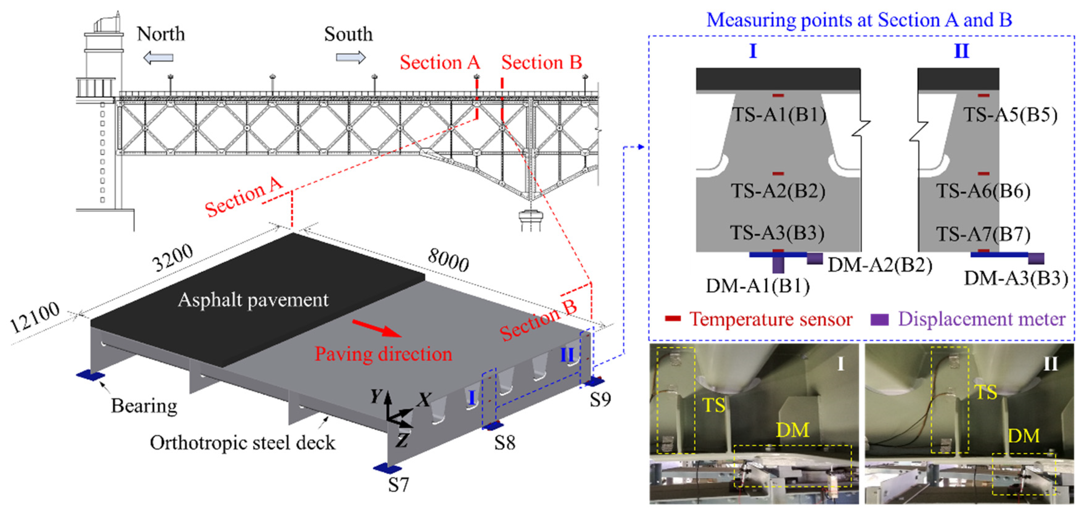
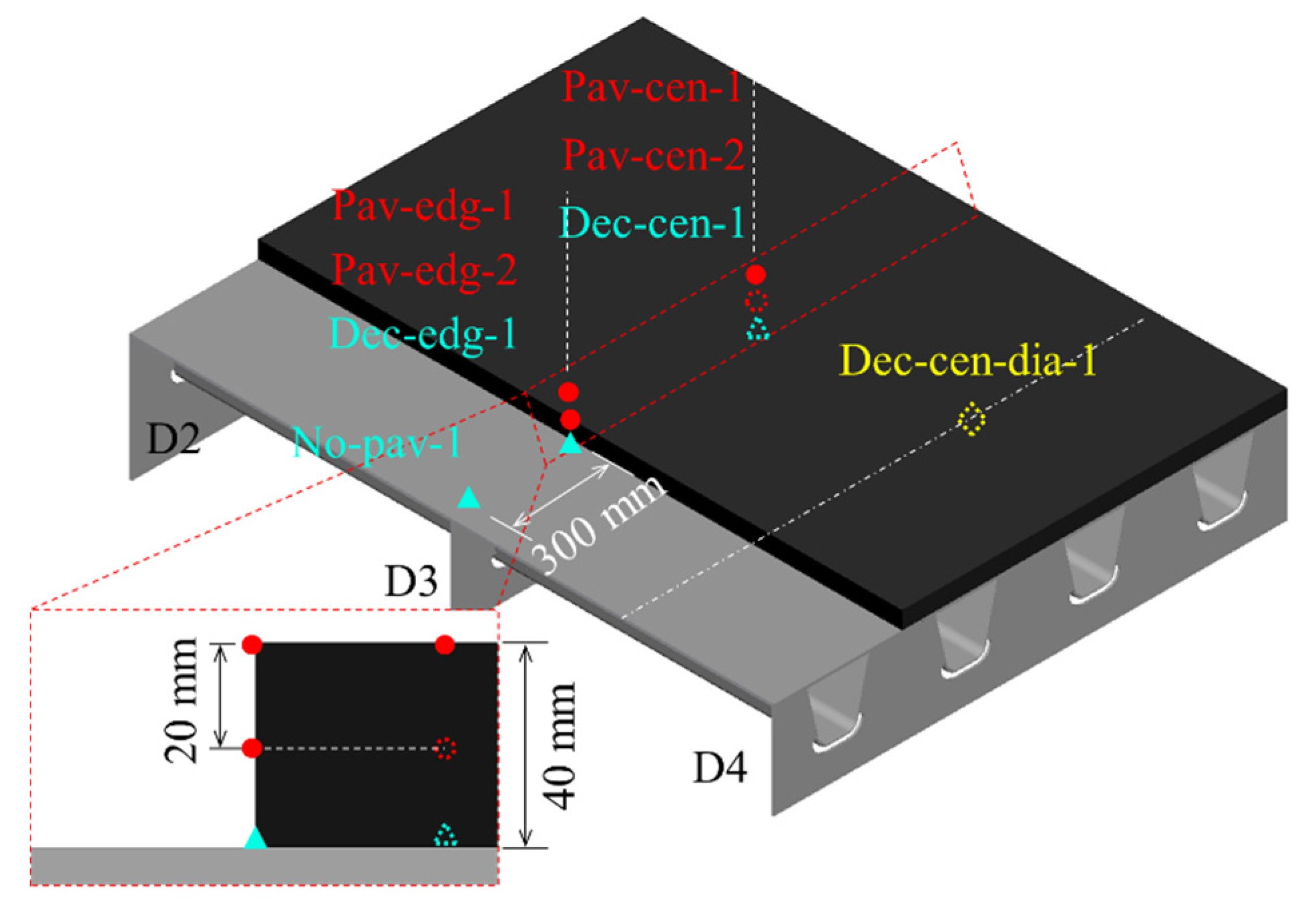
3.1. Layout of Measuring Points

Temperature of OSD and displacement of bearings were monitored during PGA paving. The asphalt surfacing to be placed on the deck plate is composed of two layers: a 40-mm-thick pouring Gaussian asphalt (PGA) concrete as the base course, and a 35-mm-thick high-elasticity modified asphalt concrete as the wearing course. In this study, the effect of PGA paving was focused on while the effect of the wearing course PGA layer was not considered. The displacement sensor typed YHD-50, which was provide by Tianjin JinAnRui Instrument Co. LTD located in Tianjin China, was adopted to monitor the displacement of the bearings. The maximum measurement value of YHD-50 is 50 mm, and the measurement accuracy is 0.01mm. Additionally, the digital temperature sensor was adopted to monitor the temperature.

One of the segments of the OSD was selected as the monitoring objective (Figure 4). The length of the segment is 8000 mm. Considering that the paving sequences would lead to temperature differences in the longitudinal direction, the temperature sensors and displacement meters were arranged at both Sections A and B, as shown in Figure 4. Additionally, four temperature sensors were also placed below the pavement centerline (TS-A4 and TS-B4) and pavement edge (TS-A8 and TS-B8) to monitor the ambient temperature. Similarly, TS-B1 to TS-B8 were arranged at the corresponding positions in Section B.

For monitoring the displacement of bearings, six displacement meters were equally arranged at each section. Taking Section A for example, both vertical and transverse displacements of the bearing below the pavement centerline (S8) were monitored by DM-A1 and DM-A2. The transverse displacement of the bearing below the pavement edge (S9) was monitored by DM-A3. Similarly, DM-B1 to DM-B3 were arranged at the corresponding positions in Section B.

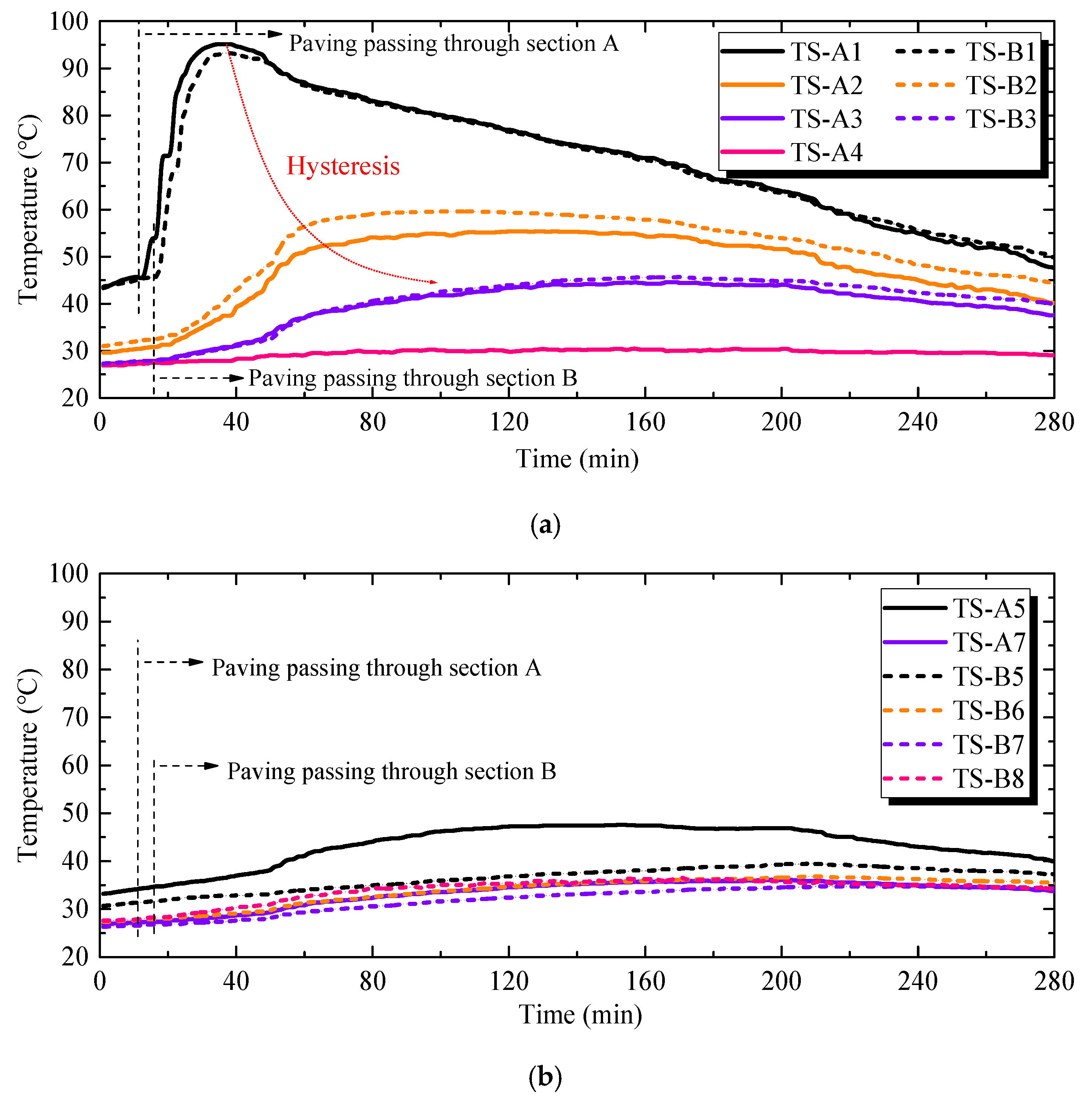
3.2. Temperature Variation during the Paving Process

All temperature sensors, excluding those monitoring ambient temperatures, were attached to the diaphragms. Hence, the monitored temperature data only represent the temperature characteristics of diaphragms. The thermal temperature variation of pavement and deck plate would be investigated based on the numerical results.

The temperature histories monitored by TS-A1 (B1) to TS-A4 (B4), which are arranged below the pavement center, are shown in Figure 5a. The temperatures at different positions of the diaphragm are affected by the vertical thermal transfer; the vertical temperature distribution of the diaphragm exhibits hysteresis during the PGA paving process. With respect to the temperatures close to the deck plate (monitored by TS-A1 and TS-B1), there is a time lag before the increase induced by the paving sequence; however, the time intervals for other measuring points are negligible due to the hysteresis induced by heat transfer. The temperatures rise quickly after PGA paving, and then decrease at a slower rate.

With respect to the temperature monitored at TS-A1, the maximum value of 95.2 °C appears at 25 min after PGA paving. The temperature monitored by TS-B1 reaches the maximum value of 93.2 °C at 22 min after PGA paving. Temperatures at the middle of diaphragm are much lower than those closest to the deck plate. Temperatures monitored by TS-A2 and TS-B2 reach their maximum values at 78 and 68 min after PGA paving, respectively. Additionally, the highest temperatures thereat are about 54.6 and 59.6 °C. TS-A4 and TS-B4 are both measuring points of ambient temperature: according to the monitored data from TS-A4, the ambient temperature near the OSDs increases from 27 to 30 °C, which is negligible. The monitored data from TS-B4 are not included in Figure 5 since it failed before PGA paving.

TS-A5 (B5) to TS-A8 (B8) were arranged below the paving edge, and the monitored data are plotted in Figure 5b. The monitored data from TS-A6 and TS-A8 are not included due to the failure of the sensors. Generally, the monitored temperatures below the pavement edge, excluding the ambient temperature, are lower than the temperatures below the pavement centerline. This could be attributable to two reasons: first, due to the transverse heat transfer, the temperature decreases gradually upon approaching the pavement edge [9]. Second, heat transfer below the pavement edge is much more complicated since there is a sidewalk closest to the pavement edge (see Figure 3). Apart from the heat transferred to the air, more heat tends to be transferred to the steel supporting the sidewalk, since steel has the greater thermal conductivity. The temperature monitored by TS-A5 reaches a maximum value of 47.3 °C at 108 min after PGA paving, however, the monitored data from TS-B5 change little, which might be due to measurement error. Meanwhile, due to the complex vertical and transverse thermal transfer, and the effect of the sidewalk, the temperatures at the middle and bottom of the diaphragm are similar.

Overall, the temperature of OSD exhibits spatiotemporal variations during high-temperature paving. The temperature at different positions on the OSD shows distinct hysteresis due to heat transfer. Uneven temperature distribution might lead to complex deformation of the OSD, which will be discussed in the following sections.

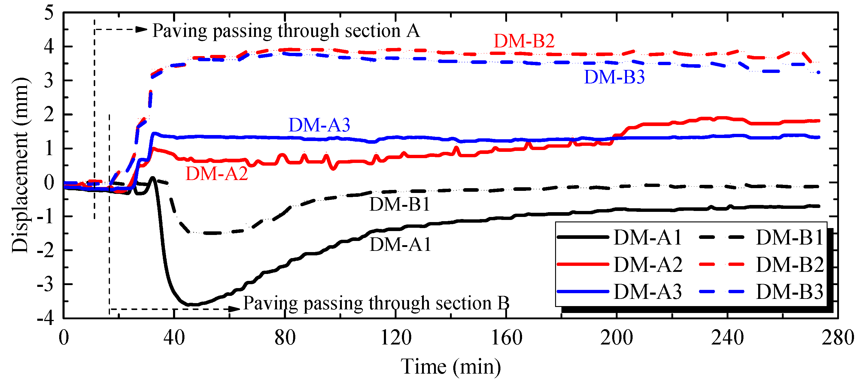
3.3. Displacement of the Bearings

As mentioned above, the bearings might be affected by high-temperature pavement paving. In in-situ monitoring, six displacement meters (DM-A1 (B1) to DM-A3 (B3)) were adopted to monitor the displacement of the bearings. The monitored data are plotted in Figure 6. Due to the thermal transfer, there is a distinct hysteresis in the displacement of the bearings (Figure 6). The displacements monitored by DM-A1 and DM-B1 are negative values, indicating local uplift deformation of the OSD. The vertical displacement increases rapidly at first until reaching its greatest value, then decreases gradually. The maximum values of the vertical displacement at Sections A and B are about 3.6 and 1.5 mm, respectively. The vertical displacement remains stable at 240 min after paving, and the residual displacements at Sections A and B are about 0.7 and 0.1 mm, respectively.

Generally, the displacement variation in the transverse direction is similar. The transverse displacements experience a rapid increasing trend at first, then remain stable (excluding data from DM-A2). The monitored data from DM-A2 still experience fluctuations at 80 min after paving, while the data monitored at DM-A3 become stable. This indicates that DM-A2 might have failed after paving. For safety and better service performance, the transverse and longitudinal displacements of tension-compression bearings (e.g., that adopted in NYRB) should be limited to no more than 5.0 and 50.0 mm, respectively. The transverse displacements of the bearings rarely decrease after reaching their maxima. According to Figure 6, the maximum value is about 4.0 mm, which is within the allowable range and indicates that the residual displacement has less effect on the service behavior of the bearings. However, the residual displacement of bearings restricts the deformation recovery of OSD, which will further lead to stress concentration at fatigable details. Such influences will be investigated in detail based on FE analysis in the following sections.

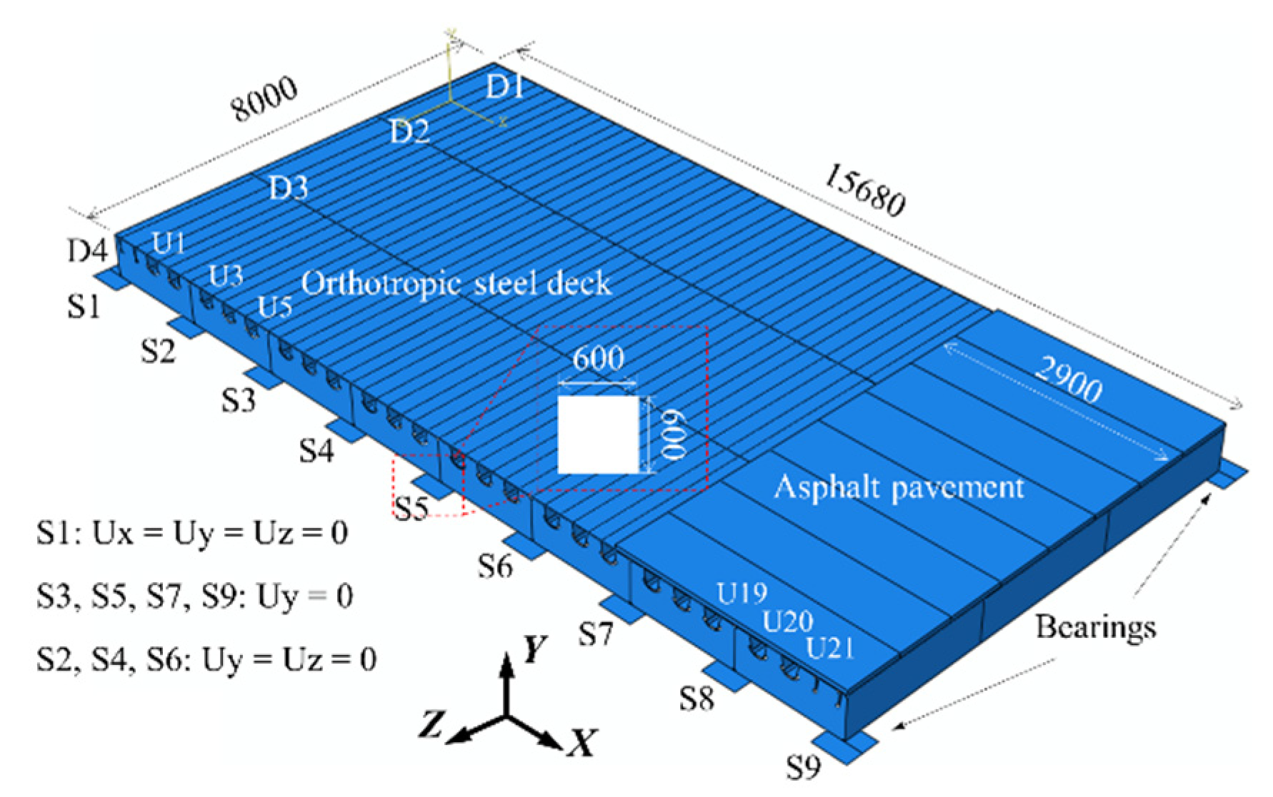
4. Modeling of High-Temperature Pavement Paving

4.1. Coupled Thermal-Structural Analysis

The residual temperature stress was analyzed based on numerical results. For this purpose, it is necessary to simulate the high-temperature pavement paving process first. In this study, the FE model for the coupled thermal-structural analysis was developed using ABAQUS. The dimensions of the model are given in Figure 7, and the FE model is shown in Figure 8. The model was composed of pavement, deck plate, base plate, 21 U-ribs (U1 to U21), four diaphragms (D1 to D4), and 18 bearings with nine at each section (S1 to S9). It should be noted that only the sublayer pavement (PGA) with a thickness of 40 mm was simulated here, neglecting the wearing course. The dimensions of the bearing were 600 (length) × 600 (width) × 20 (thickness) mm. To increase the computational accuracy, the asphalt surfacing, deck plate, U-ribs, base plate, and bearings were simulated by thermal-type solid elements (DC3D8), while the other parts were simulated by thermal-type shell elements (DS4). The global meshing size was 0.2 m, while the meshing sizes of asphalt surfacing, deck plate, bearing, and adjacent regions were refined to be 20 mm. In this case, the number of total elements and nodes are 161,195 and 229,375, respectively. The elastic modulus and Poisson’s ratio of steel were set to 206 GPa and 0.3, respectively. In the process of asphalt pavement paving, the paver can be considered as a moving heat source, thus the space–time change law of local thermal field is presented in the steel bridge deck. Hence, the thermal field of the steel bridge deck during PGA paving is treated as the transient temperature field. Hence, the element deletion approach was adopted to simulate the dynamic process of PGA paving. The simulation procedure is summarized below.

Firstly, the FEM simulating the segment of OSD was developed according to the geometric sizes. The boundary conditions and thermal parameters were applied to the FE model, which are introduced in the next section. Secondly, the pavement model was divided into 10 parts along the longitudinal direction, and all elements representing the pavement were deactivated. Subsequently, the first 10 steps were utilized to successively reactivate the pavement elements to simulate the dynamic paving process. The paving speed was controlled by the time period for each step. The paving speed of actual asphalt paver was controlled to be in the range of 2.0 to 2.5 m/min. Hence, the paving speed in the numerical simulation was set as 2.0 m/min. That is, the time period for each step was 60 s. Finally, the definition of 11 heat transfer steps was completed. The 11th step was set to simulate the temperature variation when the paving process was completed. The total calculating process lasted for 7200 s (i.e., 2 h). The solutions time was about 8 h.

The physical boundary conditions were the same with the actual situation. In NYRB, the OSD was placed on the girders using spherical tension-compression bearings, including bidirectional movable bearings, unidirectional movable bearings, and fixed bearings. Accordingly, in the numerical simulation, the displacements along the X, Y, and Z-axes of S1 were constrained to simulate the fixed bearing. The displacement along the Y-axis of S3, S5, S7, and S9 was constrained to simulate the bidirectional movable bearing. The displacement along the Y-axis and Z-axis of S2, S4, and S6 was constrained to simulate the unidirectional movable bearing.

The temperature boundary conditions were also similar to the actual environment. The temperature of OSD was determined by the coupled effect of natural convective heat transfer, solar radiation, and radiation heat transfer. Hence, the temperature boundary conditions of the asphalt surfacing and deck plate could be expressed by Equation (1) [9,13]:

$$-K{\frac{\partial T}{\partial y}|}_{y=0}=h_{c}f\left[{T_1(t)|}_{y=0}-T_a\right]+q(t)+\epsilon \sigma \left[{({T_1(t)|}_{y=0}-T_Z)}^4-{(T_a-T_Z)}^4\right]$$

(1)

where K is the thermal conductivity of the materials (58.2 W/(m·K) for steel and 1.3 W/(m·K) for pavement materials); T₁(t) refers to the temperature of different parts of the OSDs; q(t) is the intensity of solar radiation [2]; ε is the emissivity (0.4 for steel and 0.84 for pavement materials); σ is the Stefan–Boltzmann constant (5.6697 × 10⁻⁸ W/(m²·K⁴)) here; h_c is the natural convective heat transfer coefficient [2]; T_Z is absolute zero; T_a is the ambient temperature.

The effects of solar radiation and natural convention on the inner side of OSDs could be neglected. Hence, the temperature boundary conditions of the inner side of OSDs are expressed by Equation (2):

$$-K{\frac{\partial T}{\partial y}|}_{y=y_0}=\epsilon \sigma \left[{({T_1(t)|}_{y=y_0}-T_Z)}^4-{(T_a-T_Z)}^4\right]$$

(2)

Apart from the thermal boundary conditions, the specific heats of the steel and pavement were 460 and 920 J/kg·K, respectively. The densities of steel and pavement were 7850 and 2500 kg/m³, respectively. Considering that the interfacial thermal resistance between the pavement and deck plate might affect the thermal field characteristics, it was set to 2.2218 × 10⁻³ (m³·K)/W here.

The NYRB and Taizhou Yangtze River Bridge (TYRB) are close to each other. Additionally, the PGA paving for NYRB was undertaken in September, while that of TYRB was carried out in July: the corresponding ambient temperatures could be regarded as similar. Hence, the environmental thermal parameters of NYRB were referred to those of TYRB [2]. The environmental and paving parameters for thermal analysis are listed in

Table 1. Environmental and paving parameters for thermal analysis.

Parameter	Value	Parameter	Value
Solar radiation intensity (W/m2)	800	Paving temperature (°C)	230
Ambient temperature (°C)	40	Pavement thickness (mm)	40
Wind speed (m/s)	1	Paving speed (m/min)	2.0

.

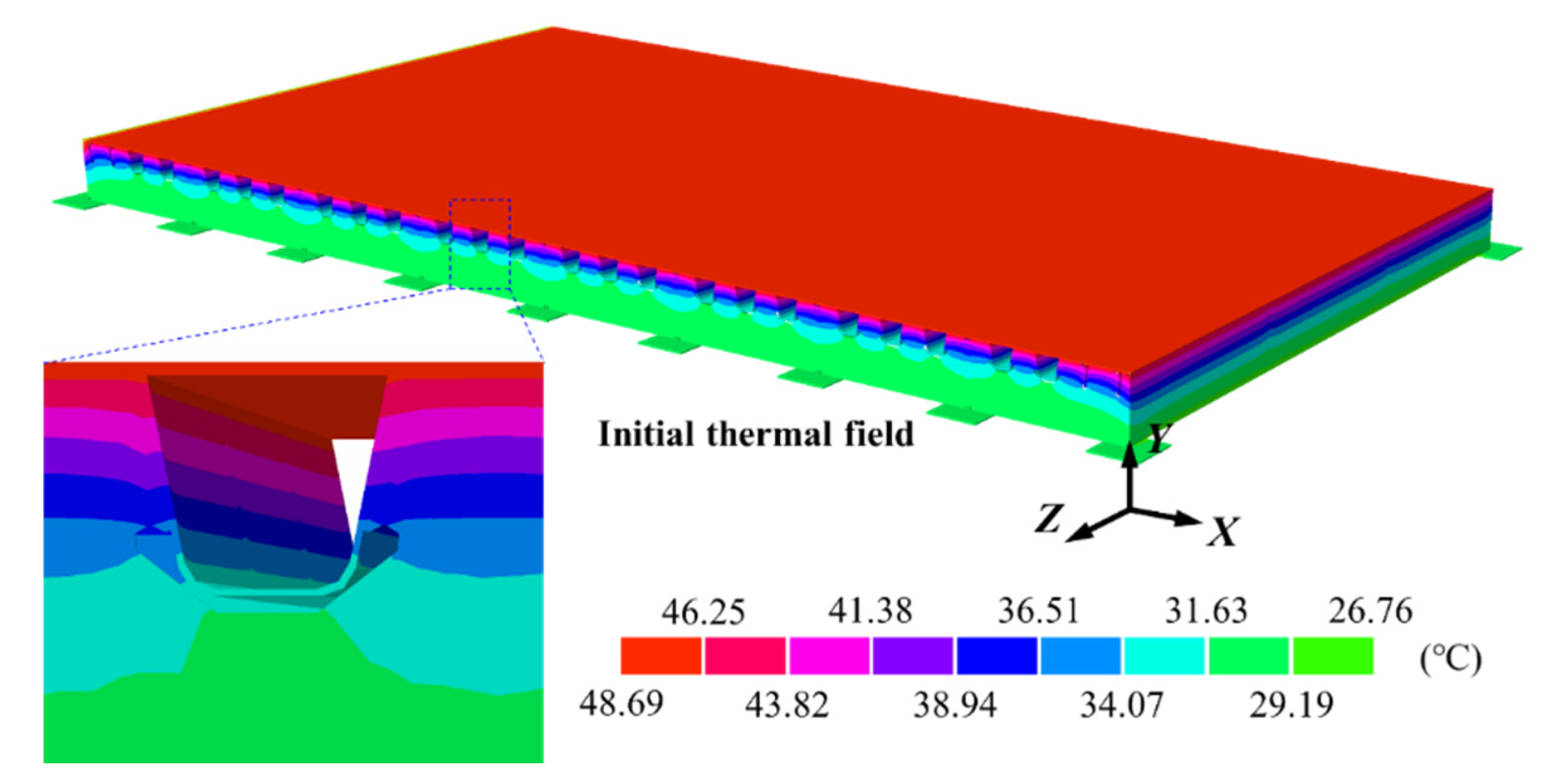
4.2. Initial Thermal Field

The initial thermal field of the OSDs was simulated before the simulation of high-temperature paving. The combined effects of ambient temperature, wind speed, and solar radiation were considered. The simulated initial thermal field is shown in Figure 9. It could be seen that the deck plate is at the highest temperature (48.69 °C). The temperature gradually decreases from the deck plate to the bearings. In in-situ monitoring, the monitored temperatures before PGA paving could be regarded as the initial temperature of the OSD. Hence, the corresponding monitored data were adopted to verify the FEM. The temperatures before PGA paving are listed in

Table 2. Comparison of initial temperatures based on monitoring and numerical results.

Measuring Point	Measured Result, tm (°C)	Numerical Result, tn (°C)	(tn − tm)/ tm × 100%
TS-A1	43.44	46.77	7.67%
TS-A2	29.71	30.88	3.94%
TS-A3	27.44	26.87	−2.08%

, where the temperatures monitored by TS-A1 to TS-A3 were adopted for comparison. The differences between the monitored and numerical temperatures are within 8%: this demonstrates that the simulated initial thermal field of OSDs is reliable.

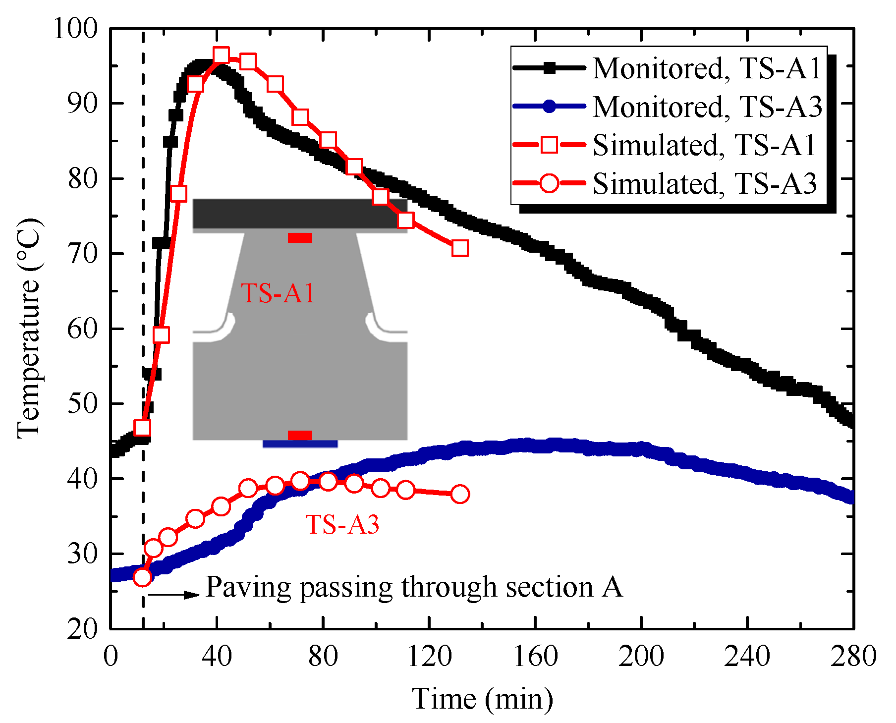
4.3. Validation of the Model

In this study, the monitored data of temperatures and displacement of bearings were both used to validate the FE model. The temperature data monitored by TS-A1 and TS-A3s were adopted to verify the model simulating this dynamic paving process (Figure 10). When the PGA paving passes through Section A, both monitored and numerical temperatures increase rapidly. The maximum values among the numerical results are very close to the monitored results. Generally, the variation in the temperature history curves is also similar. Since the objectives of this study were mainly related to the peak temperatures (e.g., the deformation of the OSDs), the minor differences (e.g., the time taken to reach the highest temperature) were believed to have less effect. Meanwhile, taking into consideration the simplification of the FE model and the measurement errors, it is deemed acceptable to conclude that the developed FE model is valid.

Figure 11 plots the numerical results of the displacements of bearings S5 to S9 at Section B, involving monitored data from DM-B2 and DM-B3. The transverse displacement gradually increases from S5 to S9. The calculated transverse displacement of S8 is 2.86 mm, 8.2% smaller than the monitored value. Meanwhile, the calculated transverse displacement of S9 is 3.54 mm, which is 9.6% greater than the monitored value. With regard to S8 and S9, the increase amplitude of numerical results is larger than that seen in monitored data. The reason for this is that the friction force within the bearings, which affects the displacements of the bearings, is neglected in the numerical simulation. However, since the difference value of monitored and numerical results is within 10%, it is also believed that the developed FE model is reliable.

5. Temperature Deformation and Stress

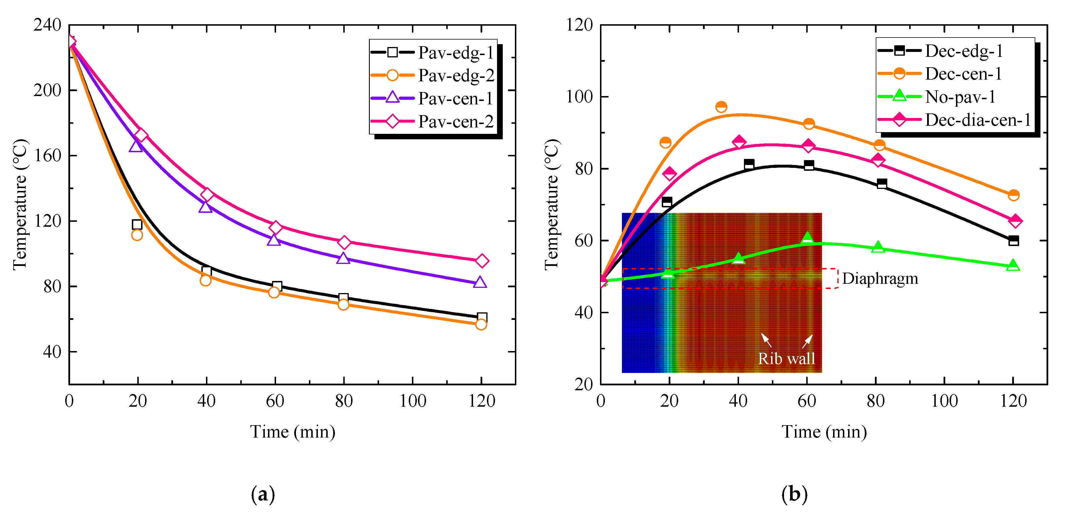
5.1. Temperature Variation at Pavement and Deck Plate

During PGA paving, the temperatures of the pavement and deck plate were not monitored. Instead, the numerical results were used to investigate the thermal characteristics, and a total of eight points were chosen (Figure 12): four points for analyzing the temperature variations on the asphalt surfacing, and another four for analyzing the temperature variations on the deck plate.

To name the specific points clearly, “Pav” and “Dec” are used to represent the points on the pavement and deck plate, respectively. “edg” and “cen” represent the edge and center of the pavement, respectively. “dia” represents the points located above the diaphragm, and “No-pav” represents points away from the paving area. Apart from Dec-cen-dia-1, which is located above D3, all points are located at the middle between D2 and D3.

The temperature histories of asphalt surfacing are plotted in Figure 13a. The initial temperature of the pavement is 230 °C, and decreases gradually after paving. The temperature at the paving edge decreases much faster at the initial stage. At about 60 min after PGA paving, the rate of decrease of the temperature at pavement edge becomes similar to that at the pavement centerline. It is also observed that the temperature at Pav-cen-2 decreases more slowly than that at Pav-cen-1, since the point lies within the asphalt surfacing.

Figure 13b plots the temperature variation at the deck plate. Generally, the temperature first increases, then decreases over time after reaching its highest value. The temperature at the pavement center (Dec-cen-1) increases faster than those elsewhere, and the highest temperature is about 96.9 °C at 35 min after PGA paving. Due to the transverse heat transfer, the temperature at the pavement edge (Dec-edg-1) reaches the highest value of 80.9 °C at 50 min after paving, which shows distinct hysteresis. Additionally, the temperature outside the paving area (No-pav-1) increases more slowly int the initial stage, and the highest temperature is 59.2 °C at 65 min after paving. Furthermore, it could be observed from the temperature nephogram (Figure 13b) that the temperature above the diaphragm and rib walls is lower. This could be attributed to the greater coefficients of thermal conductivity of the diaphragm and rib walls.

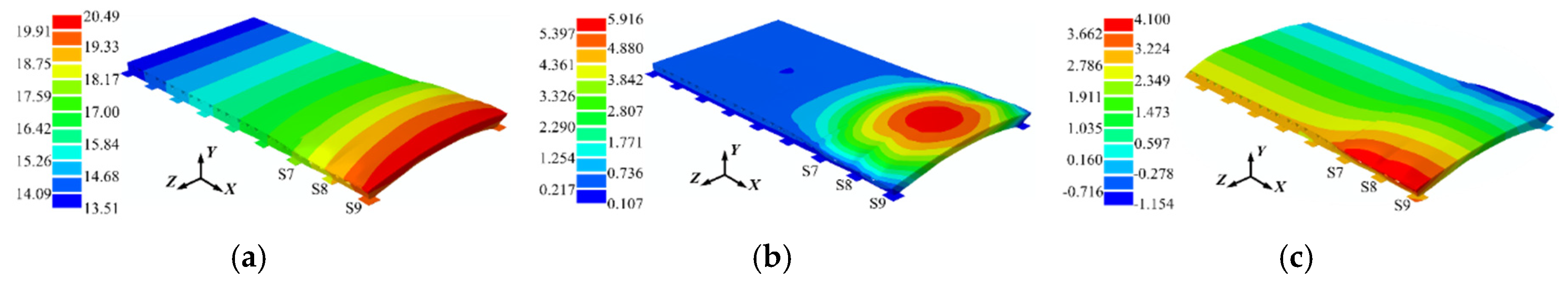
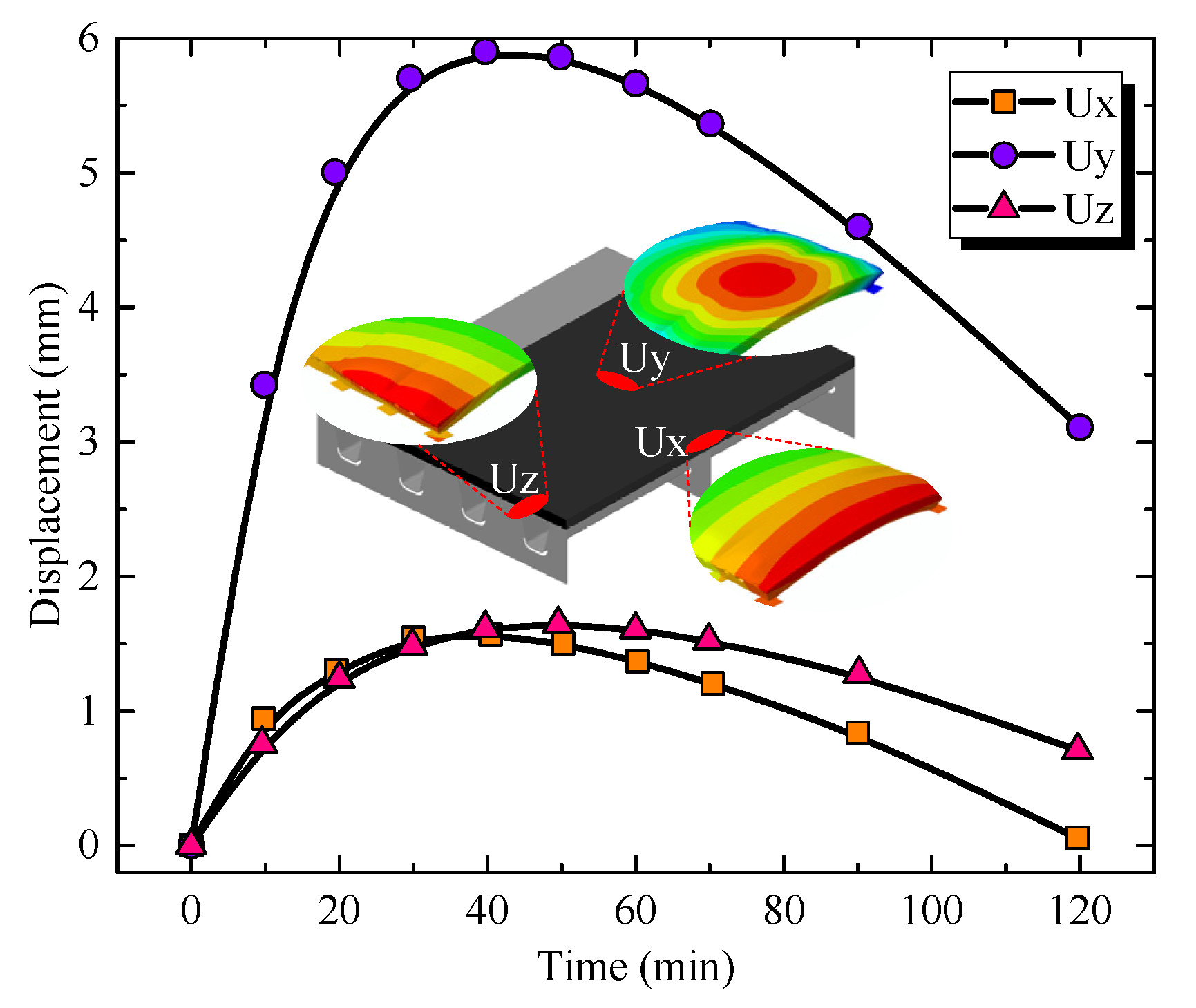
5.2. Deformation of the OSD

The thermal deformation of the OSD will occur sensibly due to the high-temperature pavement paving. The critical thermal deformation nephogram of the OSD at 40 min after paving is shown in Figure 14. The displacement–time curves at the critical positions are plotted in Figure 15. It should be noted that the values inserted in the nephogram (Figure 14) are equal to the sum of the displacements of OSD and bearings. The displacement of the OSD is the difference between the sum and that of the bearings.

As the bearing labelled S9 is transversely free, the maximum transverse displacement lies at the edge of OSD, and the maximum value is about 1.5 mm. With respect to the uplift displacement of the OSD, the maximum value appears on the deck plate in the paving area, and the maximum value is about 5.9 mm. The non-uniform uplift deformation might affect the interlayer bonding system between the pavement and deck plate. According to Figure 14c, the OSD expand in the longitudinal direction during PGA paving. The maximum displacement lies at the longitudinal end of the OSD, and the maximum value is about 1.6 mm. The displacement of the bearings and the residual temperature stress at fatigable details might be generated by the deformation of the OSD, which will be analyzed below.

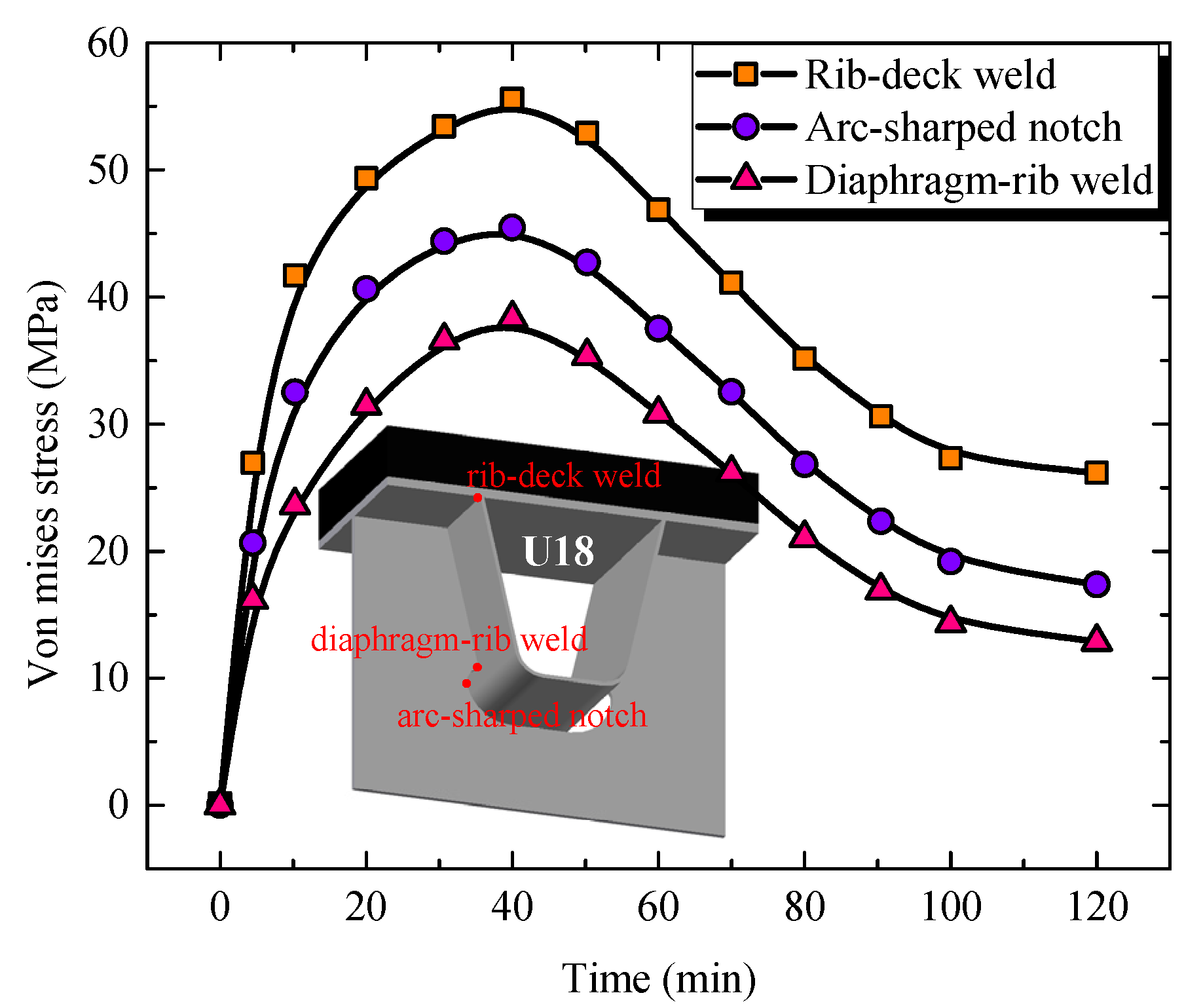
5.3. Temperature Stress at Fatigable Details

As mentioned above, there is some residual displacement of the OSD and bearings, which might result in residual stresses at fatigable details of OSD. Figure 16 shows the stress–time histories at rib-deck weld, diaphragm-rib weld, and arc-sharped notch after PGA paving. It is seen that the variation in stress is similar to that of the displacements of the OSD (Figure 15). The stress increases at first until reaching a maximum value, then decreases gradually. The temperature stress at rib-deck weld is greater than the one at other details, and the maximum value is about 55.6 MPa at 40 min after paving. The maximum stresses at arc-sharped notch and diaphragm-rib weld are 45.6 and 38.4 MPa, respectively. At 120 min after paving, the temperature stresses at rib-deck weld, arc-sharped notch, and diaphragm-rib weld decrease to 26.1, 17.3, and 12.9 MPa, respectively. This indicates that a certain value of residual stress is generated after PGA paving. Even though the residual stress is much lower than the yield strength of the base metal (e.g., 345 MPa for Q345-typed steel), it affects the mean stress at fatigable details [14], which in turn affects the fatigue performance of welds. Therefore, the effect of the residual temperature stress on the fatigue performance of fatigable details warrants further investigation.

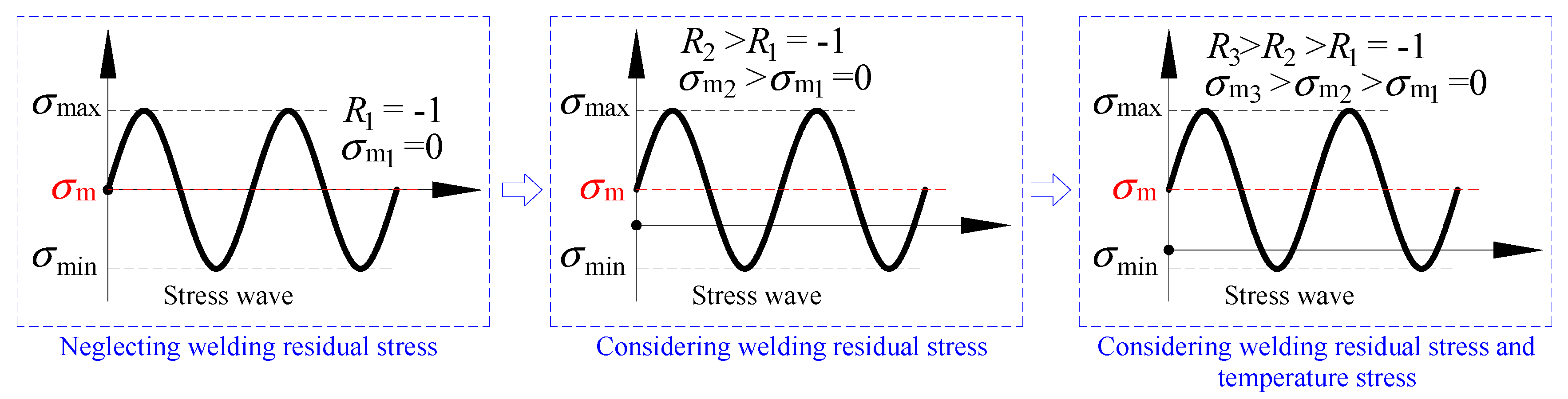
6. Fatigue Damage Evaluation Considering Residual Temperature Stress

6.1. Refining the FE Model

To investigate the effect of residual temperature stress, another FE model was developed with a 75 mm thick pavement surfacing, and the static structural analysis was carried out. The material parameters were the same with the model in Section 4.1. The asphalt surfacing is regarded as an isotropic material by assuming initial material parameters, i.e., Young’s modulus and Poisson’s ratio. The Young’s modulus and Poisson’s ratio of the asphalt surfacing was valued 1000 MPa and 0.25, respectively. The Chinese Standard “Specifications for Design of Highway Steel Bridge” was referred to for the double wheel load (60 kN), of which the loading area was 600 (transverse) × 200 mm (longitudinal) [15]. The rib-deck weld between D2 and D3 was set as the objective detail since the residual temperature stress thereof is greatest. The equivalent Von-Mises stress (σ_s) was selected as the objective stress. Actually, with regard to rib-deck weld between D2 and D3, the stress component perpendicular to the weld line (σ_x) could also be adopted, since the stress waves of σ_s and σ_x are almost overlapped with each other, as revealed in [16]. To improve the analysis precision, 20-node element typed C3D20 was adopted to simulate the OSD and asphalt surfacing. The global meshing size was set as 50 mm, while the meshing size around the objective weld was refined to be 10 mm.

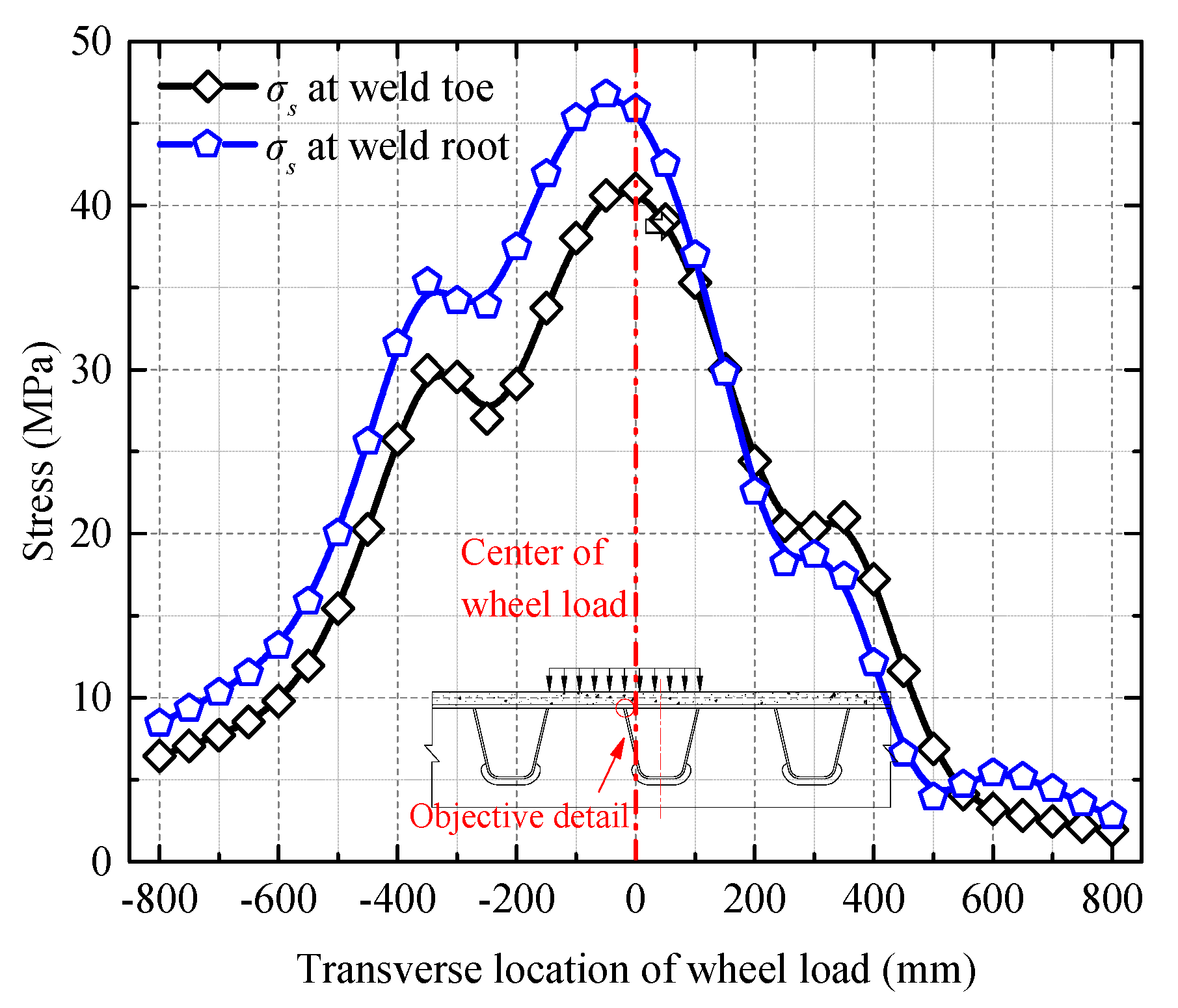
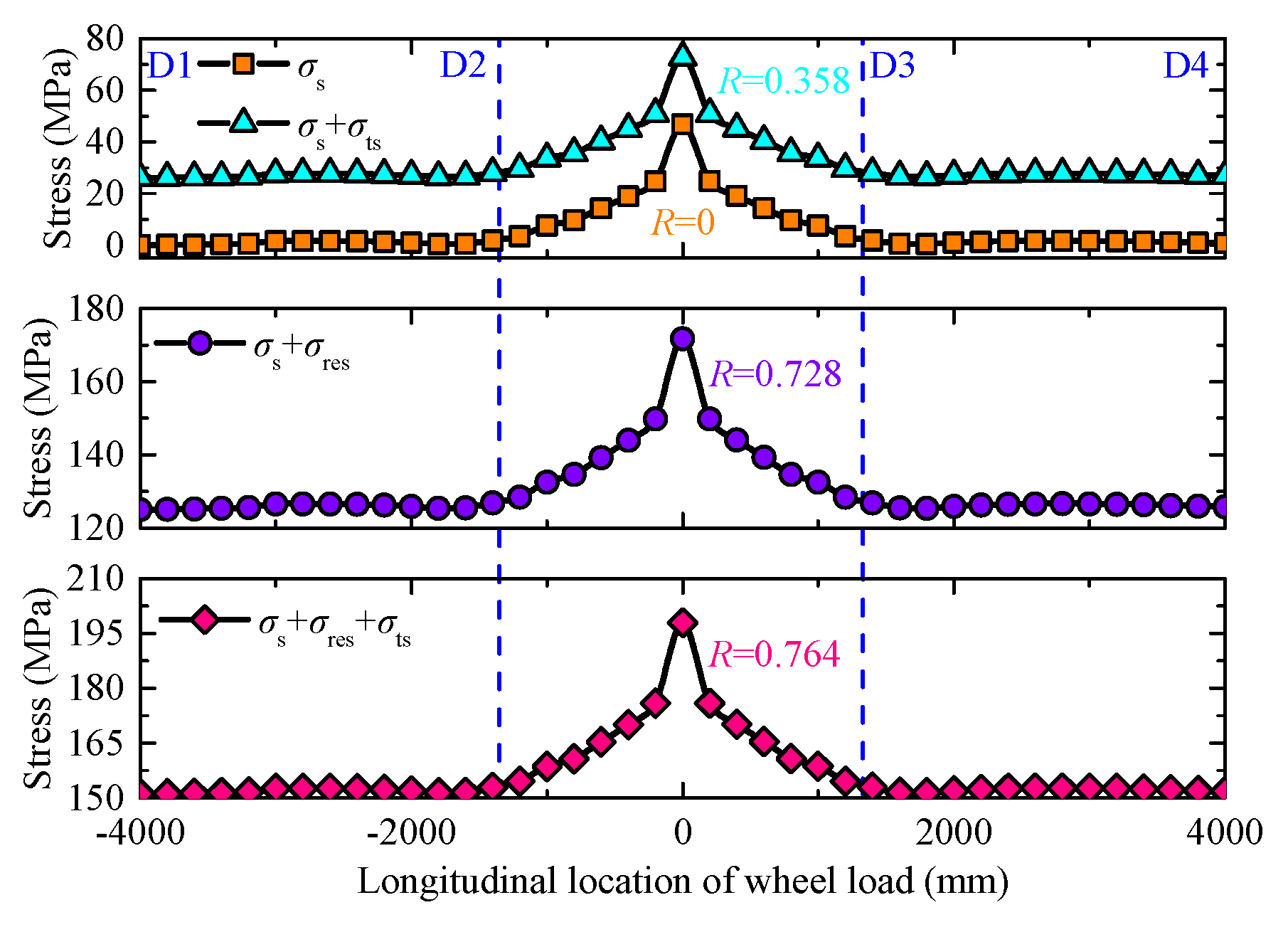
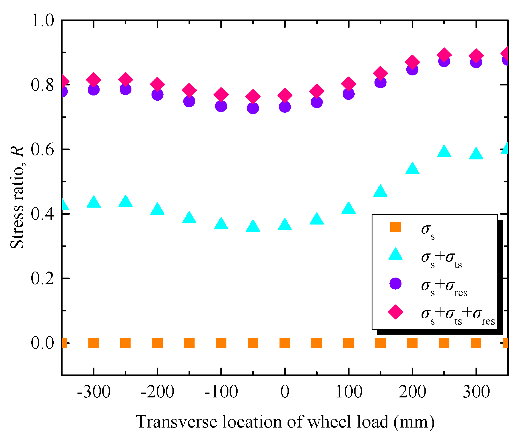
6.2. Consideration of Transverse Distribution of Wheel Load

The scatter in the transverse location of the wheel load was considered in the fatigue damage evaluation, as shown in Figure 17. Correspondingly, the transverse influence lines of rib-deck weld (Figure 18) were also obtained for ease of calculating the stress amplitude. As shown in Figure 18, the stress at weld root is generally greater than that at weld toe. It indicates that the weld root is more easily subjected to fatigue cracking. Hence, in the following analysis, the fatigue damage at weld root is focused on. Additionally, it is noted that the equivalent stress amplitude could be considered to be equal to the equivalent stress at critical loading position [17]. Therefore, the equivalent stress amplitude could be obtained from Figure 18 without calculating the stress wave.

6.3. Consideration of Residual Temperature Stress

Similar with the welding residual stress (WRS), the residual temperature stress affects the mean stress induced by wheel loads, subsequently the stress ratio. In this study, the welding residual stress at weld root was set to 125 MPa according to published data [14]. Hence, the stress wave considering residual temperature stress and welding residual stress could be obtained based on the principle of superposition of stress, as shown in Figure 19. As can be seen in Figure 19, the stress ratio (R) increases from 0 to 0.358 after considering the residual temperature stress (labelled σ_ts). Similarly, the R increases from 0 to 0.728 after considering the welding residual stress (labelled σ_res). While the coupling effect of σ_ts and σ_res is considered, the R increases from 0 to 0.764. It demonstrates that the residual temperature stress (σ_ts) affects the fatigue damage at rib-deck weld. However, it should be noted that the R given in Figure 19 only corresponds to one case of transverse location (i.e., 0 mm in Figure 17). Similar with the stress amplitude, the R also varies with the transverse location of wheel load, as plotted in Figure 20. The relative frequency of R is the same with that in Figure 17.

In this study, the Walker equation was adopted to take into consideration the effect of residual temperature stress and welding residual stress [14], as given by Equation (3):

$${\sigma }_a^{eq}={\sigma }_a{(\frac{2}{1-R})}^{1-\gamma }$$

(3)

where σ_a is the stress amplitude; ${\sigma }_a^{eq}$ is the equivalent stress amplitude; R represents the stress ratio; γ is a constant reflecting material sensitivity to mean stress, which is set to 0.7774 here.

6.4. Fatigue Damage Evaluation and Comparison

Based on the relative frequency of transverse location of wheel load, stress amplitude and stress ratio, the fatigue damage could be calculated based on Miner’s rule, as expressed by Equations (4) and (5)

$$D_i=\frac{{(\Delta {\sigma }_a^{eq})}^m}{2\times {10}^6\times \Delta {\sigma }_R^m}$$

(4)

$$D={\displaystyle {\sum }_{i=1}^n{D}_i\times P_i\times N}$$

(5)

where Δσ_R is the fatigue strength based on recommended S-N curves; the constant m is set to 3.0; P_i is the relative frequency of transverse location of wheel load (Figure 17); N is the loading cycles of single wheel per day, valued 1000 here.

To investigate the effect of residual temperature stress, four cases were considered: fatigue damage induced by wheel load only (labelled D₁); fatigue damage considering the effect of residual temperature stress (labelled D₂); fatigue damage considering the welding residual stress (labelled D₃); fatigue damage considering the coupling effect of residual temperature stress and welding residual stress (labelled D₄). Figure 21 shows the flowchart of fatigue damage evaluation process. The calculated results are given in

Table 3. Comparison of fatigue damage.

Case	D1	D2	D3	D4	(D2 − D1)/D1	(D4 − D3)/D3
Fatigue damage	7.88 × 10−5	1.09 × 10−4	1.97 × 10−4	2.17 × 10−4	38.3%	10.2%

Note: D₁ represents the fatigue damage induced by wheel load only; D₂ (or D₃) represents the fatigue damage considering residual temperature stress (or WRS) only; D₄ represents the fatigue damage considering both residual temperature stress and WRS.

. It is seen that the fatigue damage has increased by 38.3% considering the residual temperature stress only. However, since the welding residual stress is nonnegligible in real-world OSDs, the fatigue damage considering the coupling effect of welding residual stress and residual temperature stress has more practical significance. The results show that the fatigue damage considering such coupling effect has increased by 10.2%. The increased fatigue damage induced by residual temperature stress equals to that induced by 255 loading cycles (i.e., 25.5% of the total per day) of wheel load. It reveals the considerable effect of residual temperature stress on fatigue performance of OSD. Based on the numerical results, a damage amplification factor of 1.1 is recommended to represent the effect of residual temperature stress.

7. Conclusions

The influence of high-temperature pavement paving on the fatigue performance of fatigable welds was focused in this study. Both in-situ field monitoring and numerical analysis were carried out to accomplish the objectives. The following conclusions can be drawn.

(1) The temperature of an OSD exhibits spatiotemporal variations during high-temperature pavement paving. Nonuniform temperature variation leads to uplift and expanded deformation of OSD, the displacements of bearings and subsequently the temperature stress at fatigable details.

(2) Residual displacement of bearings and temperature stress at fatigable details are observed after high-temperature pavement paving. The maximum residual temperature stress appears at the rib-deck weld, indicating that the rib-deck weld is most sensitive to the high-temperature pavement paving. It is recommended to monitor the stresses at fatigable details (especially rib-deck welds) in similar projects.

(3) The stress ratio (R) increases after considering the residual temperature stress, which has considerable effect on the fatigue performance of rib-deck weld. For involving the effect of residual temperature stress, a fatigue damage amplification factor of 1.1 is suggested for similar structures.

As the monitoring data in this paper is limited, it could just represent some certain conditions. Due to some limitations, the weld stress was not monitored during high-temperature pavement paving, thus the temperature stress cannot be directly validated by the monitored data. In the future, the stress at fatigable details should also be monitored together with the temperature field.

References

1. Xiao, Z.G.; Yamada, K.; Ya, S.; Zhao, X.L. Stress analyses and fatigue evaluation of rib-deck joints in steel orthotropic decks. Int. J. Fatigue 2008, 30, 1387–1397. [Google Scholar] [CrossRef]
2. Liu, Y.; Qian, Z.D.; Hu, J.; Jin, L. Temperature behavior and stability analysis of orthotropic steel bridge deck during gussasphalt PGA paving. J. Bridge Eng. 2017, 23, 04017117. [Google Scholar] [CrossRef]
3. Memari, M.; Mahmoud, H. Performance of steel moment resisting frames with RBS connections under fire loading. Eng. Struct. 2014, 75, 126–138. [Google Scholar] [CrossRef]
4. Skriko, T.; Ghafouri, M.; Björk, T. Fatigue strength of TIG-dressed ultra-high-strength steel fillet weld joints at high stress ratio. Int. J. Fatigue 2017, 94, 110–120. [Google Scholar] [CrossRef]
5. Cao, B.Y.; Ding, Y.L.; Song, Y.S.; Zhong, W. Fatigue life evaluation for deck-rib welding details of orthotropic steel deck integrating mean stress effects. J. Bridge Eng. 2019, 24, 04018114. [Google Scholar] [CrossRef]
6. Ding, Y.L.; Zhou, G.D.; Li, A.Q.; Wang, G.X. Thermal field characteristic analysis of steel box girder based on long-term measurement data. Int. J. Steel Struct. 2012, 12, 219–232. [Google Scholar] [CrossRef]
7. Tong, M.; Tham, L.G.; Au, F.T.K.; Lee, P.K.K. Numerical modelling for temperature distribution in steel bridges. Comput. Struct. 2001, 79, 583–593. [Google Scholar] [CrossRef]
8. Kim, S.H.; Cho, K.I.; Won, J.H.; Kim, J.H. A study on thermal behaviour of curved steel box girder bridges considering solar radiation. Arch. Civ. Mech. Eng. 2009, 9, 59–76. [Google Scholar] [CrossRef]
9. Liu, Y.; Qian, Z.D.; Hu, H.Z. Thermal field characteristic analysis of steel bridge deck during high-temperature asphalt PGA paving. KSCE J. Civ. Eng. 2016, 20, 2811–2821. [Google Scholar] [CrossRef]
10. Zhou, L.R.; Xia, Y.; Brownjohn, J.M.W.; Koo, K.Y. Temperature analysis of a long-span suspension bridge based on field monitoring and numerical simulation. J. Bridge Eng. 2016, 22, 04015027. [Google Scholar] [CrossRef]
11. Xu, X.; Huang, Q.; Ren, Y.; Zhao, D.Y. Modeling and separation of thermal effects from cable-stayed bridge response. J. Bridge Eng. 2019, 24, 04019028. [Google Scholar] [CrossRef]
12. Liu, J.; Liu, Y.J.; Jiang, L.; Zhang, N. Long-term field test of temperature gradients on the composite girder of a long-span cable-stayed bridge. Adv. Struct. Eng. 2019, 22, 2785–2798. [Google Scholar] [CrossRef]
13. Rajbongshi, P.; Das, A. Estimation of residual temperature stress and low-temperature crack spacing in asphalt surfacing. J. Transp. Eng. 2009, 135, 745–752. [Google Scholar] [CrossRef]
14. Wang, Q.D.; Ji, B.H.; Chen, X.; Ye, Z. Dynamic response analysis-based fatigue evaluation of rib-to-deck welds considering welding residual stress. Int. J. Fatigue 2019, 129, 105249. [Google Scholar] [CrossRef]
15. JTG D64-2015. Specifications for Design of Highway Steel Bridge; China Communications Press: Beijing, China, 2015. (In Chinese) [Google Scholar]
16. Fu, Z.Q.; Wang, Y.X.; Ji, B.H.; Jiang, F. Effects of multiaxial fatigue on typical details of orthotropic steel bridge deck. Thin Walled Struct. 2019, 135, 137–146. [Google Scholar] [CrossRef]
17. Wang, Q.D.; Ji, B.H.; Fu, Z.Q.; Yao, Y. Effective notch stress approach-based fatigue evaluation of rib-to-deck welds including pavement surfacing effects. Int. J. Steel Struct. 2020, 20, 272–286. [Google Scholar] [CrossRef]
Figure 1. Variation of stress ratio induced by residual temperature stress.
Applsci 10 07196 g001
Figure 2. Research flow chart.
Applsci 10 07196 g002
Figure 3. High-temperature pavement paving in the reconstruction of Nanjing Yangtze River Bridge (NYRB) (Images taken by Q.W.).
Applsci 10 07196 g003
Figure 4. Arrangement of temperature sensors and displacement meters (unit: mm).
Applsci 10 07196 g004
Figure 5. Variation of monitored temperatures. (a) TS-A1 (B1) to TS-A4 (B4); (b) TS-A5 (B5) to TS-A8 (B8).
Applsci 10 07196 g005
Figure 6. Monitored displacement of the bearings during the paving process.
Applsci 10 07196 g006
Figure 7. Geometric sizes of the model (unit: mm).
Applsci 10 07196 g007
Figure 8. Finite element (FE) model as built (unit: mm).
Applsci 10 07196 g008
Figure 9. Initial thermal field of OSD before PGA paving.
Applsci 10 07196 g009
Figure 10. Comparison of monitored and numerical results of temperature.
Applsci 10 07196 g010
Figure 11. Comparison of monitored and numerical results of displacement of bearings.
Applsci 10 07196 g011
Figure 12. Arrangement of extracting points.
Applsci 10 07196 g012
Figure 13. Variation of simulated temperatures. (a) Pavement surfacing; (b) deck plate.
Applsci 10 07196 g013
Figure 14. Deformation nephogram of the OSD (amplification factor: 400). (a) Ux; (b) Uy; (c) Uz.
Applsci 10 07196 g014
Figure 15. Variation of the maximum displacement of OSD along X-, Y-, and Z-axes.
Applsci 10 07196 g015
Figure 16. Variation of the stress at fatigable welds during the paving process.
Applsci 10 07196 g016
Figure 17. Transverse distribution of the wheel load.
Applsci 10 07196 g017
Figure 18. Stress influence lines of rib-deck weld.
Applsci 10 07196 g018
Figure 19. Stress wave at weld root under critical loading position.
Applsci 10 07196 g019
Figure 20. Stress ratio corresponding to different transverse loading positions
Applsci 10 07196 g020
Figure 21. Flowchart of fatigue damage evaluation procedure.
Applsci 10 07196 g021