Diagnostics 101: A Tutorial for Fault Diagnostics of Rolling Element Bearing Using Envelope Analysis in MATLAB

Abstract

This paper presents a MATLAB-based tutorial to conduct fault diagnosis of a rolling element bearing. While there have been so many new developments in this field, no studies have addressed the tutorial aspects in this field to help the engineers learn the concept and implement by their own effort. The three most common techniques—the autoregressive model, spectral kurtosis, and envelope analysis—are selected to demonstrate the bearing diagnosis process. Simulation signal is introduced to help understand the characteristics of fault signal and carry out the process toward the fault identification. The techniques are then applied to the two real datasets to demonstrate the practical applications, one made by the authors and the other by the Case Western Reserve University, which is known as a standard reference in testing the diagnostic algorithms.

1. Introduction

Prognostics and Health Management (PHM), which enables life extension while preventing unexpected failures in various engineering systems, have received great attention over the last decades for more efficient operation and maintenance. Generally, there are three main steps in the PHM development: (1) signal processing, (2) diagnosis, and (3) prognosis. Signal processing is the step in which the valuable information called features are extracted from noisy sensor signals such as vibrations or acoustic emissions. Diagnosis focuses on detecting the faults, isolating their locations, and identifying their severity based on the extracted features. Lastly, the prognosis is to predict the Remaining Useful Life (RUL) based on the accumulated diagnostic information, which indicates how long it will take until the system’s health reaches the failure threshold. Though the most important step is the prognosis, its performance is of no doubt dependent on the quality of prior steps: the signal processing and the diagnosis.

To date, the PHM has mainly focused on the vibration signal-based techniques for rotating mechanical components such as gears [1,2] and bearings [3,4,5,6,7], since they usually lead to the critical failures [1,8]. Among them, the rolling element bearings, which support the shaft during the rotation, have been of greatest importance in view of its widespread use and often cause of another failures. For example, the bearings are known to cause around 70% of gearboxes and 21–70% of generator failures in the wind turbine industries [9]. To prevent such failures, early fault detection and diagnosis of the bearings is important. A great deal of research has been conducted on this topic. Many review papers are available, addressing the state-of-the-art algorithms from various perspectives. Only a few are given here; among others, Rai et al. reviewed several signal processing techniques for the rolling element bearing fault diagnosis [10]. Cerrada et al. have reviewed fault severity assessment methods [11]. Hamadache et al. made review on artificial intelligence-based approaches including shallow and deep learning [12]. Reviews are available, too, on the bearings for specific applications; Caesarendra et al. presented feature extraction methods for the low-speed slew bearing [13]. de Azevedo et al. have reviewed condition monitoring methods for bearings in the wind turbine [9].

As such, a great number of new algorithms have been introduced and reviewed over the last decades. Despite the importance, however, no studies have dealt with the tutorial aspects except the one by Randall and Antoni, which have introduced a number of techniques covering the essential as well as advanced algorithms in the context of diagnostic procedure [14]. The paper was highly informative and enlightening in several aspects, but it was in some sense close to a collection of their recent achievements in a single article, and hence was less instructive in view of the self-explanatory aspects of the tutorial. In real practice, there are many instances that engineers without enough knowledge in this field fail to solve their problems due primarily to the lack of detailed understanding of the algorithms and of how to implement them. Motivated by this, a tutorial is presented in this paper to conduct the fault diagnosis of rolling element bearing, with the purpose to help the beginners learn by themselves the basic concepts along with implementing the algorithms with minimum resort to the external resources.

Among the techniques currently available for the bearing diagnosis, envelope analysis is the most common and relatively well established, which enables to detect the fault with location by matching the frequency spectrum of the envelope to the fault frequencies. By the way, the bearing signal is usually masked by the resonant noise and those coming from other components (e.g., gears and engines), which should be filtered out as a first step. Spectral kurtosis and autoregressive model are the most commonly applied techniques for this purpose [14]. These are addressed in the context of diagnosis process using the MATLAB scripts.

Simulation datasets are prepared to explain the characteristics of the raw signal and the process of how to retrieve the fault information out of it. The techniques are then applied to the real datasets made by the authors to demonstrate the practical applications. The datasets by the Case Western Reserve University, which have been a standard reference in testing the diagnostic algorithms, are also used to demonstrate the general nature of the techniques.

The paper is organized as follows. In Section 2, the basic theory and procedures in the bearing diagnostics are introduced. Section 3 addresses how to implement the bearing diagnosis using the simulation data. Practical diagnoses using the MATLAB codes are also performed with the real datasets in Section 4 and Section 5. Lastly, conclusions are presented in Section 6.

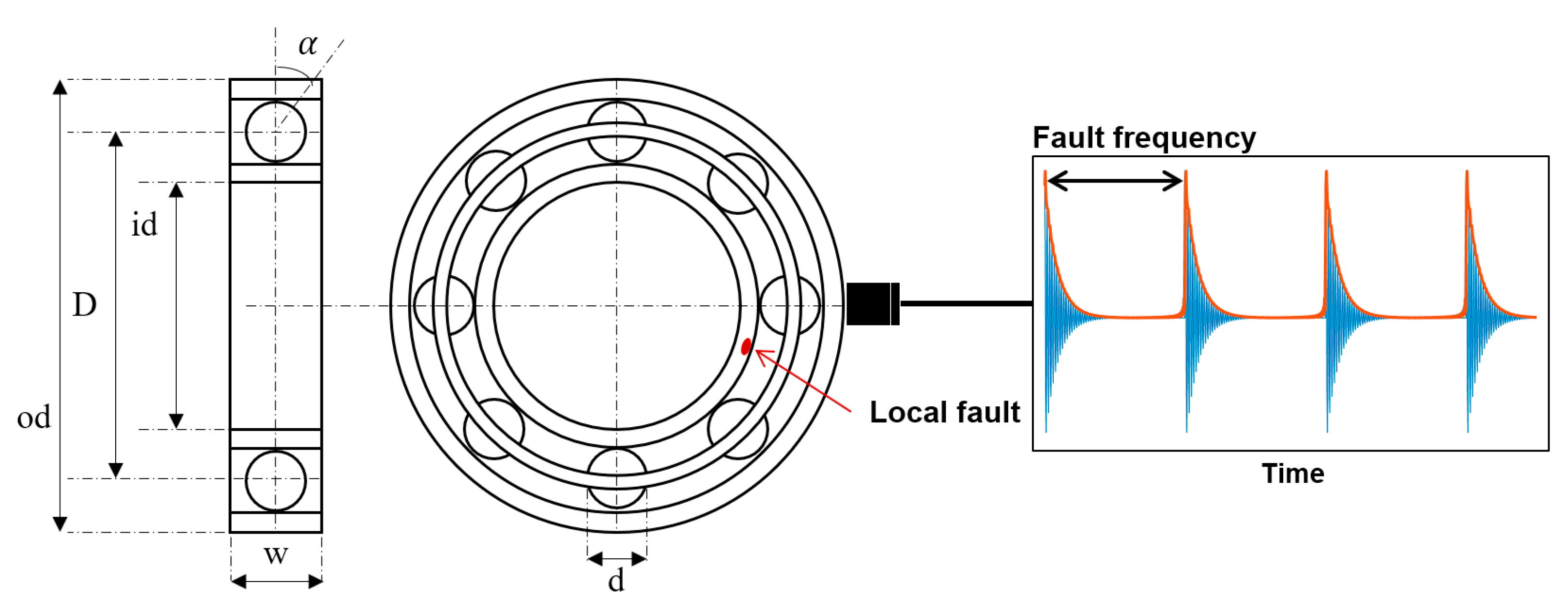
2. Bearing Diagnostics

In this section, fundamental characteristics of fault signal is addressed first in view of amplitude modulation. Then, a virtual signal is generated to illustrate what the real signal is like in terms of its components, which will be used in implementing the diagnosis procedure in the next section.

2.1. Fault Signal Given by Amplitude Modulation

Whenever the rolling element in the bearing strikes a local fault in the inner or outer race or vice versa during operation, an impact signal is produced at the period of one of the bearing fault frequencies, such as Ball Pass Frequency Outer race (BPFO), Ball Pass Frequency Inner race (BPFI), Fundamental Train Frequency (FTF), and Ball Spin Frequency (BSF), which are defined as follows [15].

$$BPFO = \frac{n{f}_s}{2}\left\{1+\frac{d}{D}cos\alpha \right\}$$

(1)

$$BPFI = \frac{n{f}_s}{2}\left\{1-\frac{d}{D}cos\alpha \right\}$$

(2)

$$FTF = \frac{f_s}{2}\left\{1-\frac{d}{D}cos\alpha \right\}$$

(3)

$$BSF = \frac{D{f}_s}{d}\left\{1-{\left(\frac{d}{D}cos\alpha \right)}^2\right\}$$

(4)

where 𝐷, 𝑑, 𝛼, 𝑛 and $f_s$ are the pitch diameter, ball diameter, contact angle between the ball and the cage, number of rolling elements, and the rotating speed of bearing (Hz), respectively. Usually, the impact signals at these fault frequencies are modulated by the much higher resonant frequencies of the bearings, which results in the signal like the one in Figure 1, the exponentially decaying ringing occurring periodically at the fault frequencies [16].

This phenomenon is mathematically the same as the amplitude modulation (AM), of which the concept is illustrated by a simple example in Figure 2. The fault and the resonance signal of the bearings are assumed to be Figure 2a,b which are the modulating and carrier signal in the signal processing theory, respectively. Then, the AM signal becomes the carrier signal with variable amplitude given by the modulating signal as shown in Figure 2c. After taking the FFT, the frequency domains of modulating, carrier, and the AM signals are given in Figure 2e–g, respectively. The result shows that the AM spectrum has peaks at the resonance (carrier) frequency ($f_r$) with the sidebands spaced apart by the fault (modulating) frequency ($f_f$) [17]. The AM signal can be expressed by the following equation [18]:

$$x\left(t\right) = \left[1+f\left(t\right)\right]\times r\left(t\right) = \left\{1+Msin\left(2\pi f_{f}t\right)\right\}Acos\left(2\pi f_{r}t\right)$$

(5)

where f(t) is the fault signal (plus DC offset to ensure that the mean amplitude of AM signals is zero) with the amplitude M and frequency $f_f$, r(t) is the resonance signal with the amplitude $A$ and frequency $f_r$, and $x\left(t\right)$ is the AM signal. Equation (5) can be transformed to

$$x\left(t\right) =Acos\left(2\pi f_{r}t\right)+\frac{A·M}{2} \left[sin2\pi \left(f_r+f_f\right)t-sin2\pi \left(f_r-f_f\right)t\right]$$

(6)

which shows that the spectrum of the AM signals consists of three components $f_r$, $f_r\pm f_f$, with the amplitudes $A$ and $A$·$M/2$, respectively, as shown in Figure 2f. Therefore, it can be concluded that, when a bearing has fault, it appears as the sideband around the resonance signal. Then, the remaining task is to extract or separate the original fault signal Figure 2a or its FFT (e) from the AM signal Figure 2c or its FFT (g). This is realized by the envelope analysis, which is an amplitude demodulation technique as will be addressed in the subsequent section.

2.2. Simulation of Fault Signal

With this understanding, more complex signal closer to the reality is considered. Toward this end, a virtual signal is generated using the MATLAB code given in Appendix A. A fault signal is created as shown in Figure 3a by an exponential function, $x_1\left(t\right)=A\cdot exp\left(-\alpha t^{\prime }\right)$ to represent the transient impact signal with the frequency $f_f=10$ Hz, where $t^{\prime }=mod\left(t,1/f_f\right)$ and A and $\mathsf{\alpha }$ represent the magnitude of impulse signal and the damping parameter of the bearing, respectively. They are given by 5 and 75.4 in this example. The mod stands for the modulus after division, which is to make repeated signal over time [19]. The FFT of this signal becomes Figure 3d, where the fundamental frequency is 10 Hz with amplitude 1.0 with the subsequent ones being its harmonics. This is modulated by a carrier signal given by the sinusoidal function $x_2\left(t\right)=sin\left(2\pi f_{r}t\right)$ with frequency $f_r=600$ Hz which is much higher than $f_f$, as shown in Figure 3b–c. This corresponds to the resonance of the bearing. Then, the modulated signal becomes $x_3\left(t\right)=x_1\left(t\right)\ast x_2\left(t\right)$, and is shown in Figure 3c in which the carrier contains the fault in its amplitude [20]. Its FFT becomes Figure 3f, where the sidebands are present around 600 Hz.

Added to this, the signal may include a certain discrete signals from other components such as gears and shafts as well as the background noise. In this example, they are represented by another low-frequency sinusoidal function $x_4\left(t\right) = sin\left(2\pi f_{d}t\right)$ with amplitude 2 and frequency $f_d=13\mathrm{Hz}$ and Gaussian white noise $x_5\left(t\right)~N\left(0,{\sigma }^2\right)$ with variance ${\sigma }^2 = {0.5}^2$, which are given by Figure 4a,b, and their FFTs (d) and (e), respectively. Putting all these together, the resulting raw signal $x\left(t\right) = x_3\left(t\right)+x_4\left(t\right)+x_5\left(t\right)$ becomes Figure 4c with its FFT being (f). Note that the governing sinusoidal wave shown in Figure 4c is the discrete signal $x_4$. The amplitudes at the high-frequency region in Figure 4f represent the carrier at 600 Hz (resonance) and surrounding sidebands (faults), which is a more complex version of the AM mentioned in Figure 2. The frequency amplitudes of the discrete and AM signal are 2 and 0.6, respectively, which means that the fault is buried by the carrier and another discrete signals. This agrees with the finding that the signals from the gears and shafts often show higher amplitudes than those of faulty bearing; typically, the amplitudes of the shaft rotation, gear meshing and the bearing fault signals are on the order of 0.1, 10 and 0.001 g [21,22].

3. Diagnosis Using Simulation Data

The goal of the diagnosis is to isolate the fault information from the raw signal mixed with other noisy sources. The steps are taken in reverse order of the way the virtual raw signal is made and are summarized in Figure 5. It consists of three steps: First is the discrete signal separation to remove signals from the other components. Second is the demodulation band selection to find out the band containing resonance frequencies, using which the band pass filtering is carried out to obtain only the signal in the band while removing those elsewhere. Last is the envelope analysis to restore the original fault signal out of the modulated signal around the resonance frequencies. Usually, the first two steps are denoted as the signal pre-processing. Note that the raw signal includes the mixture of four signals: bearing fault signal, resonance signal, and discrete signal with frequencies $f_f$,$f_r$ and $f_d$ and the background noise.

Regarding the algorithms in each step, autoregressive (AR) models are applied [14,23] for the discrete signal separation at first. Spectral kurtosis (SK) and Short Time Fourier Transform (STFT) are employed in the second step to select frequency band where the bearing resonance is dominant. In the third step, Hilbert transform is applied for the envelope analysis to obtain the analytic signal. Then, its magnitude becomes the envelope signal. By taking the FFT of the envelope signal, the fault information is retrieved from the amplitudes at the fault frequencies. More details are explained in the following sub-sections. MATLAB code with 63-lines is provided in the Appendix B to implement the process, which consists of four parts: (1) problem definition, (2) discrete signal separation, (3) demodulation band selection, and (4) envelope analysis.

3.1. Problem Definition (Lines 1–7)

In the code, six parameters are required in the problem definition. The first four are related to the data acquisition and bearing dimensions, and thus should be fixed for the same applications. Raw data are stored in the variable rawData. Simulation data generated by Appendix A are loaded into this variable. The parameters sampRate, rpm and bearFreq denote the sampling rate in Hz, shaft rotation speed in rpm and bearing fault frequency. Note that there are four fault frequencies in the bearing, which are calculated by the Equations (1)–(4) based on the shaft frequency in rpm and bearing specifications. In the simulation, however, a single fault frequency is directly assigned, which is $f_f = 10$ Hz as shown in Figure 3a. Therefore, the rpm is just set at 60 here. The last two parameters maxP and windLeng are to control the performance of the algorithm: maxP is the maximum order of the AR model, which is given by 300 from the ratio of the sampRate = 3000 and bearFreq = 10. This is based on the criteria that the model order should not be greater than the number of data within a fault interval [23]. The parameter windLeng is a row vector of the lengths in the window function of STFT. In this example, four different window lengths [2^4 2^5 2^6 2^7] are used. More details about how to set optimum window length can be referred to in Ref. [24].

3.2. Discrete Signal Separation (Lines 8–22)

The first step is the discrete signal separation that removes the signals from the other sources such as gears and shafts, which we call the discrete (deterministic) signal. The discrete signal can be obtained by the autoregressive (AR) model, which is to estimate the current value of time series data via weighted sum of the past values. Then, the residual signal is obtained by subtracting the AR model, i.e., the discrete part, from the raw signal, as shown in Figure 6.

Let us consider a time series x(n) with n = 1, N, which is the raw vibration signal acquired with sampRate per seconds. The AR model is then constructed to predict the next value in a time series by using a series of previous observations, which is described by the following equation [22] (line 15):

$$x_p\left(n\right) = -{{\displaystyle \sum }}_{k = 1}^{p}a\left(k\right)x\left(n-k\right)\mathrm{or}\mathrm{in}\mathrm{a}\mathrm{matrix}\mathrm{form}{x}_p=-Xa$$

(7)

where $x_p\left(n\right)$ is the predicted value at nth time step as a weighted sum of its p previous values in the sequence, p is the order of the model, a(k) is the weighting coefficients, and x(n-k) is n-kth data. The matrix $X$ is an $N\times p$ matrix consisting of the past series values of $x$ (line 13–14). The coefficient $a\left(k\right)$ can be obtained by solving the Yule–Walker equation [14,22] (line 12):

$$\left[\begin{array}{cccc}{r}_{xx}\left(0\right)& r_{xx}\left(-1\right)& \cdots & r_{xx}\left(-p+1\right)\\ r_{xx}\left(1\right)& r_{xx}\left(0\right)& \cdots & r_{xx}\left(-p+2\right)\\ ⋮& ⋮& \ddots & ⋮\\ r_{xx}\left(p-1\right)& r_{xx}\left(p-2\right)& \cdots & r_{xx}\left(0\right)\end{array}\right]\left[\begin{array}{c}a\left(1\right)\\ a\left(2\right)\\ ⋮\\ a\left(p\right)\end{array}\right]=-\left[\begin{array}{c}{r}_{xx}\left(1\right)\\ r_{xx}\left(2\right)\\ ⋮\\ r_{xx}\left(p\right)\end{array}\right]$$

(8)

where $r_{xx}\left(k\right)$ is the autocorrelation function of x(n), which is defined by

$$r_{xx}\left(k\right) = \frac{1}{N}{\displaystyle \sum }_{n = 1}^{N}x\left(n\right)x\left(n-k\right), k = 0,\dots ,p-1$$

(9)

In order to illustrate the process, an example is given when p = 2. Then, Equation (8) becomes

$$\left[\begin{array}{cc}{r}_{xx}\left(0\right)& r_{xx}\left(-1\right)\\ r_{xx}\left(1\right)& r_{xx}\left(0\right)\end{array}\right]\left[\begin{array}{c}a\left(1\right)\\ a\left(2\right)\end{array}\right] = -\left[\begin{array}{c}{r}_{xx}\left(1\right)\\ r_{xx}\left(2\right)\end{array}\right]$$

(10)

where

$$r_{xx}\left(0\right) = \left[x\left(1\right)x\left(1\right)+x\left(2\right)x\left(2\right)+\cdots +x\left(N\right)x\left(N\right)\right]/N$$

$$r_{xx}\left(1\right) = \left[x\left(1\right)x\left(0\right)+x\left(2\right)x\left(1\right)+x\left(3\right)x\left(2\right)\dots +x\left(N\right)x\left(N-1\right)\right]/N$$

$$r_{xx}\left(-1\right) = \left[x\left(1\right)x\left(2\right)+x\left(2\right)x\left(3\right)+\cdots +x\left(N-1\right)x\left(N\right)+x\left(N\right)x\left(N+1\right)\right]/N$$

$$r_{xx}\left(2\right) = \left[x\left(1\right)x\left(-1\right)+x\left(2\right)x\left(0\right)+x\left(3\right)x\left(1\right)\dots +x\left(N\right)x\left(N-2\right)\right]/N$$

In the equations, the items $x$ exceeding the range [1, N] do not exist, hence, are assigned zero. Then, the AR model at nth step becomes by Equation (7)

$$x_p\left(n\right) = -a\left(1\right)x\left(n-1\right)-a\left(2\right)x\left(n-2\right)$$

(11)

Once the deterministic signal $x_p$ is obtained from the AR model, the residual signal is obtained by subtracting the prediction from this (line 16).

Since the order p affects the prediction performance, it should be determined to make the residual signal represent the fault as best as it can. Depending on its uses, there are several different criteria to determine the order p, such as Akaike information criteria (AIC) [25,26,27,28], Bayesian information criterion (BIC) [29], Minimum description length (MDL) [30], and Partial Autocorrelation Function (PACF) [31]. In the bearing fault diagnosis, the order p is usually determined such that the kurtosis of the residual signal is maximized, as are addressed in many literatures (e.g., [23]). The latter is used here because it is simpler to calculate and the kurtosis is the impulsiveness indicator of fault signal. For this objective, the kurtosis is calculated by increasing the order p from 1 to maxP = 300 (lines 10–18). The result is in Figure 7a, where the maximum is at p = 82, hence, is used for optP (line 19). Then, the AR model is constructed again using this, which is to repeat lines 12–15. In this case, however, it is implemented by the MATLAB function filter, which does the same but in more simple way (line 21). Residual signal thus obtained can be plotted by entering plot(rawData.t (optP+1:end),e) in the MATLAB command window, and is shown in Figure 7b along with its kurtosis value. Additionally, the raw signal and its kurtosis are given in Figure 7c for comparison. Kurtosis is higher by about four times after removing the discrete signals, reflecting the fault presence more clearly. For more advanced results, however, another criteria as mentioned above may be applied to determine the model order p and choose the one with better performances after comparison. This may be beyond the scope of this paper.

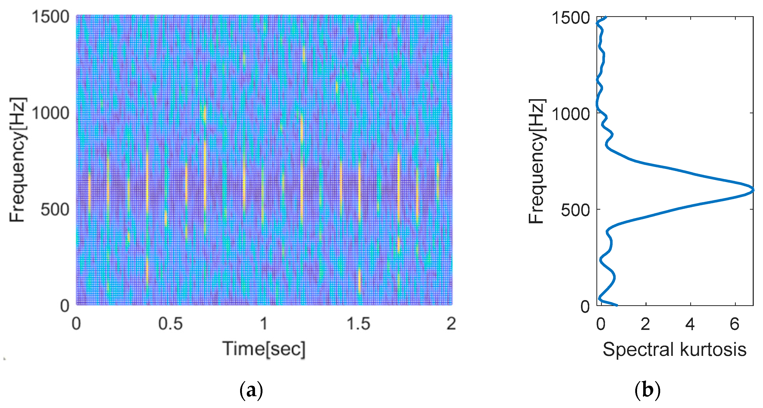
3.3. Demodulation Band Selection (Lines 23–49)

As the second step of the signal pre-processing, a frequency band enclosing the resonance frequencies is sought from the residual signal. It is determined based on the spectral kurtosis (SK), which is the kurtosis at each frequency line in a time- frequency diagram. When the fault occurs, the SK becomes higher around the region of resonance frequencies onto which the fault signal is modulated. The SK is defined by the functions of short time Fourier transform (STFT) [14,32] (line 39):

$$K\left(f\right) = \frac{{\langle \left|S\left(t,f\right)\right|}^4\rangle }{{\langle \left|S\left(t,f\right)\right|}^2\rangle {}^2}-2$$

(12)

where 〈⋅〉 is the time-averaging operator, and S(t,f) is the STFT of the residual signal. The STFT is a local Fourier transform for a finite time window at time t, which varies from $t =0$ to $t_{\mathrm{end}}$ (lines 27–37). The process is illustrated in Figure 8, in which the top figure is the raw signal, and middle figure is the window function to restrict the signal to the range at each time point t = t₀ ~ t_w, from which the local signals are made as shown in the figures below. Then, one obtains the bottom figure by taking the Fourier transform for each signal. Among various window functions, this paper employs the Hann window as follows with length L [24] (line 27):

$$w\left(l\right) = 0.5\left(1-cos\left(2\pi \frac{l}{L-1}\right)\right), 0\le l\le L-1$$

(13)

The time interval of Fourier transform is given by the half of the window length. Remembering that the sampling rate of the signal is 3000 Hz, which means 3000 data are in a second, when the window length is 2⁷ = 128; for example, the first signal at $t_0$= 0 in the middle figure resides in the range of 0$\le t\le 0.0427(1\le n\le 128$), and the second at $t_1 = 0.0213 \left(n = 65\right)$, in the range of $0.0213\le t\le 0.0640(65\le n\le 192$), etc.

The results of FFT in Figure 8 can also be plotted in the 2D form called spectrogram, as shown in Figure 9a, which shows the frequency spectrum where the x and y axes are the time and frequency. Finally, the SK can be computed using Equations (1) and (2) to obtain as a function of frequency, as shown in Figure 9b (lines 38–40). Based on the figure, the frequency range for high SK can be selected visually, which is around 400-800 Hz in this case (lines 43–47). The frequency band thus obtained is used to band-pass filter the residual signal, which leaves only the spectrum in the band (lines 48–49).

By the way, the results of STFT may vary by different window lengths, which leads to the different SK. For better results, it is necessary to set a proper window length in the STFT. In case the fault interval can be identified visibly as is found as 0.1 s ($n = 300$) in Figure 7b, it is advised that the length be smaller to some degree than the number of data within the interval, which is the same as maxP. In practice, however, since the signal is not so clear, several window lengths are usually attempted [14], which are in this example given arbitrarily by [2^4 2^5 2^6 2^7] (line 7). Upon obtaining the SK with each window lengths (lines 26–42), they are plotted in superposition (line 45), from which the frequency band for higher SK is visually determined (lines 47). The result is shown in Figure 10a, where demodulation bands are set between [500 700] for the range of higher kurtosis in common. This should be input in the command window as shown in Figure 10b. Then, the residual signal goes through band-pass filtering to result in the signal in Figure 10c of which the kurtosis increases by twice to 23.1865 from 10.5885.

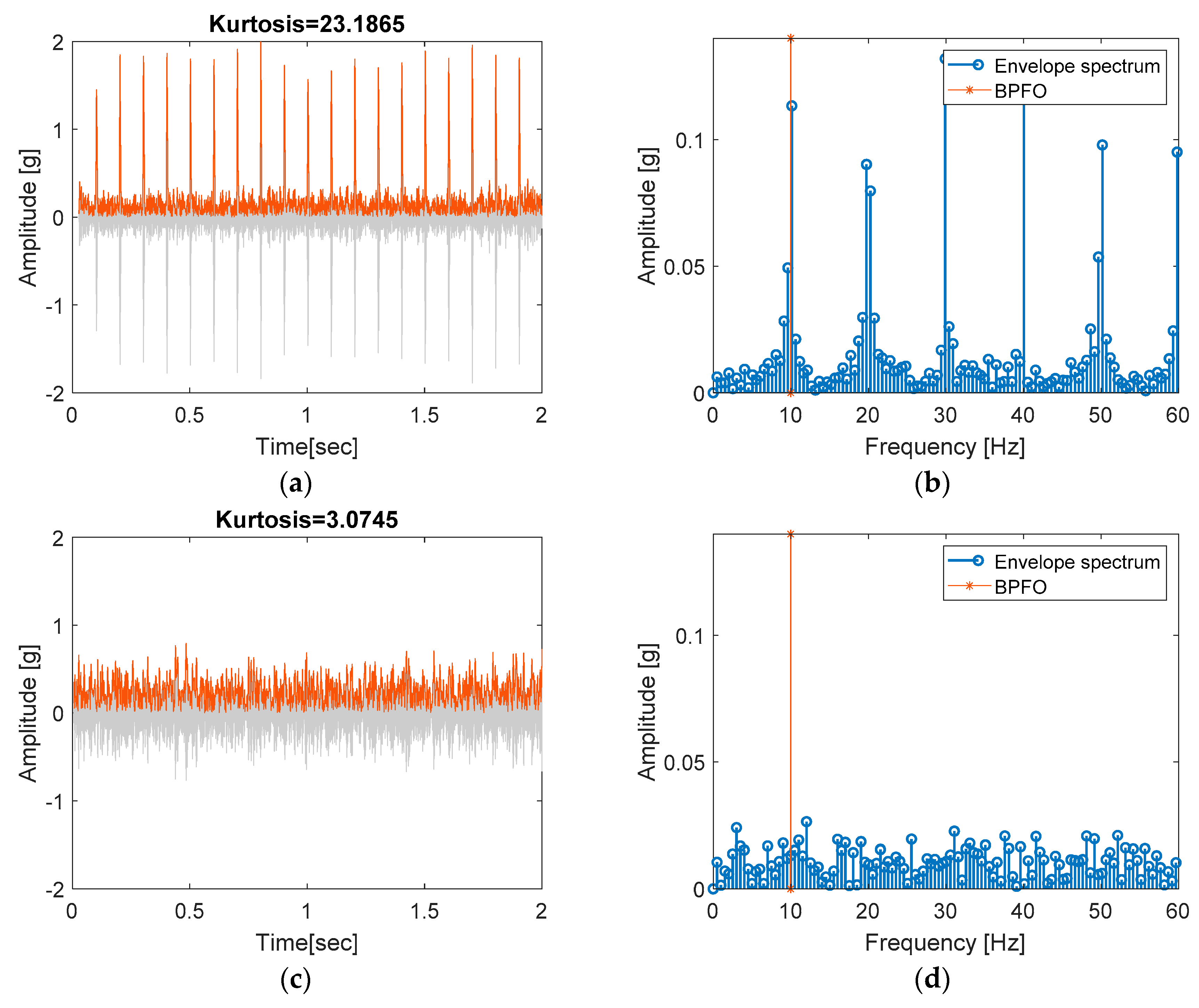
3.4. Envelope Analysis (Lines 50–64)

After two pre-processing techniques—discrete signal separation and band-pass filtering—one obtains the AM signal that includes only components of resonance (carrier) and fault (modulation) frequency. Then, the envelope analysis is used as the last step for the diagnosis of bearing faults, which consists of three sub-steps: First, Hilbert transform is applied to the AM signal to obtain the analytic signal [14,15,17] (line 51). Next, its magnitude is calculated to obtain the envelope signal, which is the absolute value of the analytic signal (line 52). It is further translated to have zero mean by removing the DC offset (line 53). Last, FFT is taken to the envelope signal to retrieve the fault information from the amplitudes at the fault frequencies (lines 54–55).

The Hilbert transform is referred to as a 90° phase shifter and results in the analytic signals, expressed as follows [18]:

$$a_x\left(t\right) = x\left(t\right)+j\widehat{x}\left(t\right) = \sqrt{x^2\left(t\right)+{\widehat{x}}^2\left(t\right)}{e}^{j{\varphi }_x\left(t\right)} = A_x\left(t\right)e^{j{\varphi }_x\left(t\right)}$$

(14)

where $a_x$ indicates the analytic signal, in which the real part $x$(t) is the original AM signal, imaginary part $\widehat{x}\left(t\right)$ is its Hilbert transform, ${\varphi }_x\left(t\right)$ is the instantaneous phase, and $A_x$ is the instantaneous amplitude, i.e., the envelope signal. The resulting envelope signal with the DC offset is shown in Figure 11a. The envelope spectrum after taking FFT is given in Figure 11b, in which the fault is identified by examining the amplitude at the given fault frequencies (lines 56–64). In the figure, the peaks near the fault frequency 10 Hz and its harmonics are apparent, which indicates that the fault has occurred indeed. Compare the Figure 11a,b with the original ones in Figure 3a,d to find out that result of the envelope spectrum is different, which we call smearing. The reason is because the sampling rate is low and the length of residual signal is changed from the original one after the AR filtering. Though not addressed here, it is left to the reader to implement and figure out what the result will be when the fault is small or nonexistent by assigning smaller value to A. For comparison, envelop analysis results of healthy bearing are also given in Figure 11c,d, which can be easily made by assigning A = 0 in the MATLAB code (Bearing fault simulation). Comparing Figure 11a,b with the fault, the normal bearing does not show periodic impulse representing the fault in the time domain and the peak at the fault frequency in the frequency domain either. Furthermore, the kurtosis value is about 3 in the normal bearing, which is much smaller than that of fault and the typical of the Gaussian distribution.

4. Diagnosis of Korea Aerospace University (KAU) Bearing Faults

In this section, diagnosis is performed using the real vibration data made by the authors’ test rig in the Korea Aerospace University (KAU). It is shown in Figure 12 which consists of DC motor, support bearings, and two roller bearings for the test. Vertical load is applied to the support bearing. The test bearing is given by NSK NJ 2306, with its geometry and dimensions in

Table 1. Bearing dimensions.

Parameter Name	Value	Parameter Name	Value
Bearing type	NJ 2306	Width (w)	27 mm
Inner diameter (id)	30 mm	Dynamic load rating	51,500 N
Outer diameter (od)	72 mm	Static load rating	51,000 N
Number of rollers (n)	11

. Fault is seeded at the inner race with an artificially induced notch (0.2 mm depth, 0.3 mm width). The accelerometer is installed on top of the test bearing’s housing using bolt to acquire the vibration signals. The test is performed under four different conditions as listed in

Table 2. Operating conditions.

Data Name	RPM	LOAD
bearing 1	1200 rpm	0 N
bearing 2	1200 rpm	200 N
bearing 3	1000 rpm	0 N
bearing 4	1000 rpm	200 N

.

In order to diagnose the bearing fault, the fault frequencies as stated in Equations (1)–(4) should be available. In practice, however, most of the bearing manufacturers do not provide the values of ball and pitch diameter. To solve this problem, a commercial bearing fault frequency calculator [33] is adopted in this study and the results are listed in

Table 3. Bearing fault frequencies.

Frequency Name	Value	Frequency Name	Value
BPFO	$4.4423\times f_r$	FTF	$0.4038\times {\mathrm{f}}_{\mathrm{r}}$
BPFI	$6.5577\times f_r$	BSF	$5.0079\times {\mathrm{f}}_{\mathrm{r}}$

$f_r:\mathrm{shaft}\mathrm{rotating}\mathrm{speed}$ [Hz].

. The bearing data are acquired through a sampling frequency of 51.2 kHz.

In order to illustrate the process, the dataset for “bearing 1” is taken, which is operated with a rotating speed of 1200 rpm and a 0 N vertical load (note that the load by the weight of bearing housing still exists). Figure 13 shows the raw signal, of which the kurtosis is 4.9923. The four datasets listed in Table 2 can be downloaded from https://www.kau-sdol.com/ and https://sites.google.com/view/sg-kim.

The raw data for bearing 1 are loaded by the name bearing1. Referring to Table 2, sampRate and rpm are set at 51.2e3 and 1200, respectively. Bearing fault frequencies are assigned in bearFreq, which is [4.4423 6.5577 0.4038 5.0079] for BPFO, BPFI, FTF, and BSF, respectively, based on Table 3. The maximum order of the AR model maxP is set at 390 based on the ratio of the sampling frequency versus the highest fault frequency (51200/(6.5577*1200/60)) as mentioned before. Vector of the window lengths windLeng for STFT are given by [2^4 2^5 2^6 2^7 2^8] under the constraint of maximum length being smaller than maxP (390). As a result, the commands in the Problem definition (lines 1–7) are modified as follows:

-

Line 2: rawData = load('bearing1');

-

Line 3: sampRate = 51.2e3;

-

Line 4: rpm = 1200;

-

Line 5: bearFreq = [4.4423 6.5577 0.4038 5.0079]*rpm/60;

-

Line 6: maxP = 390;

-

Line 7: windLeng = [2^4 2^5 2^6 2^7 2^8].

After going through the discrete signal separation (lines 8–22), one obtains the optimum order optP being 318 for the AR model by maximizing the kurtosis of the residual signal. Then, the resulting residual signal becomes Figure 14 and its kurtosis is 44.0245, roughly a nine-fold increase. Demodulation band selection (lines 23–49) is then carried out using the four sets of SK made with five window lengths, which are given in Figure 15a. The proper frequency band for higher SK is selected by visual examination of this figure, which is given arbitrarily as [1.8e4 2.3e4] by the authors. The residual signal after applying band-pass filter is then obtained as shown in Figure 15b, of which the kurtosis increases to 208.849, five times greater than the previous one.

After typing in the frequency band, it continues to the envelope analysis (lines 50–64), and the results are shown in Figure 16. In the figure, the four fault frequencies are plotted as vertical lines, at which the peak is examined to identify whether the fault has occurred or not. The result, however, should be interpreted with caution. It shows multitude of peaks at the several frequencies: the first group is at the shaft frequency (20 Hz = 1200 rpm/60 s) and its harmonics (black arrows), which can be caused by unbalance, misalignment, or coupling lock up. Details associated with shaft harmonics can be referred to the literature [34]. Next is at the BPFI (130 Hz) and sidebands with harmonics spaced at the interval of shaft frequency (20 Hz) around it (orange arrows). Once the peaks like these are identified around the BPFI, it indicates the inner race fault occurrence. Note that, in case of inner race fault, sidebands typically appear around the BPFI, whereas it is not so in the other faults [35]. Note also that sometimes the peaks can overlap by chance in the same frequency range, as is found at BPFO, which should not be mistaken as the fault.

5. Diagnosis of CWRU Bearing Faults

Vibration data provided by the Case Western Reserve University (CWRU) Bearing Data Center are employed [36,37] to demonstrate another application of the diagnosis code. In this case, artificial faults ranging in diameter from 0.007 to 0.028 inches were seeded with the electro-discharge machining (EDM) on drive-end (SKF 6205-2RS JEM) and fan-end (SKF 6203-2RS JEM) bearings. During the tests, data were collected at 12 and 48 kHz sampling rates for several datasets. Test bearings were driven with different rotation speeds ranging from 1797 to 1720 rpm. Accelerometers were installed on three different locations: on the drive-end bearing (DE), the fan-end bearing housing (FE), and the motor supporting base plate (BA).

Among others, this paper considers the bearing with inner race fault on the fan end. Geometry information and fault frequencies of the bearings are listed in

Table 4. Bearing information.

Parameter Name	Value	Parameter Name	Value
Pitch diameter (D)	1.122 inch	BPFO	3.0530$f_r$
Ball diameter (d)	0.2656 inch	BPFI	4.9469$f_r$
Number of rolling element (n)	13	FTF	0.3817$f_r$
Contact angle ($\mathsf{\alpha }$)	0	BSF	1.994$f_r$

(the number of rolling elements and contact angles are not provided directly, and they are calculated by using the suggested fault frequencies), and the sampling rate and rotation speed are 12 kHz and 1796 rpm, respectively. The data are also available with the name “bearing 270” (the original data was resaved with two variables: vib for vibration data, and t for measuring time in rawData) at https://www.kau-sdol.com/. Further details regarding the data and test rig can be found in references [36,37].

Based on the information provided by the literature, the code to test the bearings is changed as follows:

-

Line 2: rawData = load (‘bearing270’);

-

Line 3: sampRate = 12e3;

-

Line 4: rpm = 1796;

-

Line 5: bearFreq = [3.053 4.947 0.382 1.994]*rpm/60;

-

Line 6: maxP = 82;

-

Line 7: windLeng = [2^4 2^5 2^6].

In line 6, since the highest fault frequency is BPFI with 148.0802 Hz (4.947*1796/60), the maximum order of the AR model should be 82 (12000/148.0802), which is the number of data within a fault interval. In line 7, window lengths are set based on the criteria mentioned in Section 3.3. The results are shown in Figure 17. Based on the visual inspection of spectral kurtosis in Figure 17a, [5.3e3 5.9e3] Hz is selected in the command window for the demodulation band selection. After band-pass filtering by this interval, the results of the envelope analysis are shown in Figure 17b, which shows a dominant peak at BPFI (148.08 Hz) and sidebands with harmonics at the interval of shaft frequency (29.93 Hz), convincing that the bearing has inner race fault.

As a supplementary explanation, the effects of each step in the signal preprocessing are also demonstrated in Figure 18, in which the envelope analysis are carried out to the raw signal (a) and to the residual signal that went through the AR filtering (b), respectively. In Figure 18a, the peak at BPFI in the spectrum is apparent but is smaller than the others, which is doubtful of the fault. Another peak appeared at BSF (59.69 Hz) also does not give us the confidence because it coincides with the harmonic of shaft frequency, which are the multiples of 29.93 Hz. After the AR filtering, the peak at the BPFI is increased greatly along with the sidebands with the intervals of shaft frequency in Figure 18b. This confirms the fault at that frequency. On the other hand, the height at the BSF is not changed relative to the neighbors, which suggests that it may not be the fault but the harmonic of the shaft frequency. In this case, the fault at BPFI is already identified at this step without further preprocessing, i.e., the demodulation band selection, although the result may be better interpreted as shown in Figure 17b. As such, not all bearings have to resort to the full preprocessing steps for the fault identification.

Refer to the following code to obtain the results in Figure 18.

• aX = hilbert(rawData.vib); %=== (a) Raw signal
• envel = abs(aX);
• envel = envel-mean(envel);
• fftEnvel = abs(fft(envel))/Ne*2;
• fftEnvel = fftEnvel(1:ceil(N/2));
• freq = (0:Ne-1)/Ne*sampRate;
• freq = freq(1:ceil(N/2));
• figure(3)
• stem(freq,fftEnvel,’LineWidth’,1.5); hold on;
• [xx,yy] = meshgrid(bearFreq,ylim);
• plot(xx(:,1),yy(:,1),’*-’,xx(:,2),yy(:,2),’x-’,xx(:,3),yy(:,3),’d-’,xx(:,4),yy(:,4),’^-’)
• legend(‘Envelope spectrum’,’BPFO’,’BPFI’,’FTF’,’BSF’);
• xlabel(‘Frequency [Hz]’); ylabel(‘Amplitude[g]’); xlim([0 max(bearFreq)*1.8])
•  
• aX = hilbert(e); %=== (b) Residual signal
• envel = abs(aX);
• envel = envel-mean(envel);
• fftEnvel = abs(fft(envel))/Ne*2;
• fftEnvel = fftEnvel(1:ceil(N/2));
• figure(4)
• stem(freq,fftEnvel,’LineWidth’,1.5); hold on;
• [xx,yy] = meshgrid(bearFreq,ylim);
• plot(xx(:,1),yy(:,1),’*-’,xx(:,2),yy(:,2),’x-’,xx(:,3),yy(:,3),’d-’,xx(:,4),yy(:,4),’^-’)
• legend(‘Envelope spectrum’,’BPFO’,’BPFI’,’FTF’,’BSF’);
• xlabel(‘Frequency [Hz]’); ylabel(‘Amplitude [g]’); xlim([0 max(bearFreq)*1.8])

6. Conclusions

Signal processing for feature extraction is an important step in the fault diagnosis and prognosis, but the process in detail are not fully understood for the beginners of PHM to implement by themselves. With this motivation, this paper has presented a tutorial for how to identify the fault using the envelope analysis along with the preprocessing steps such as AR filtering and SK filtering to remove the unnecessary signals and noises, which are widely used in the area of bearing fault diagnostics. MATLAB codes for the algorithms are provided, which consists of 64 lines and can be simply modified for the other applications. Two sets of bearing vibration data (data made by the authors and CWRU bearing data) are used to help the user to implement and understand the algorithms. The code and bearing data are available at https://www.kau-sdol.com/ and https://sites.google.com/view/sg-kim. Apart from the datasets in this tutorial, there are several more datasets open to the public, and some of those are listed in

Table 5. Open Data for Fault Diagnosis and Prognosis of Bearings.

Data Set Name	Diagnosis	Prognosis	Failure Type	Operating Condition
FEMTO [38]	X	O	Natural	Different load and speed
MFPT [39]	O	X	Artificial	Different load
IMS [40]	X	O	Natural	Single condition
WT [41]	X	O	Natural	Single Condition
Paderborn [42]	O	X	Artificial, Natural	Different operating condition

to help the user practice diagnosis themselves.

References

1. He, D.; Bechhoefer, E.; Ma, J.; Zhu, J. A particle filtering based approach for gear prognostics. In Diagnostics and Prognostics of Engineering Systems: Methods and Techniques; IGI Global: Hershey, PA, USA, 2013; pp. 257–266. [Google Scholar]
2. Kim, S.; Choi, J.H. Convolutional neural network for gear fault diagnosis based on signal segmentation approach. Struct. Health Monit. 2019, 18, 1401–1415. [Google Scholar] [CrossRef]
3. An, D.; Choi, J.H.; Kim, N.H. Remaining useful life prediction of rolling element bearings using degradation feature based on amplitude decrease at specific frequencies. Struct. Health Monit. 2018, 17, 1095–1109. [Google Scholar] [CrossRef]
4. Siegel, D.; Ly, C.; Lee, J. Methodology and framework for predicting helicopter rolling element bearing failure. IEEE Trans. Reliab. 2012, 61, 846–857. [Google Scholar] [CrossRef]
5. Kim, S.; Park, S.; Kim, J.W.; Han, J.; An, D.; Kim, N.H.; Choi, J.H. A new prognostics approach for bearing based on entropy decrease and comparison with existing methods. In Proceedings of the Annual Conference of the Prognostics and Health management Society, Denver, CO, USA, 3–6 October 2016. [Google Scholar]
6. Lim, C.; Kim, S.; Seo, Y.H.; Choi, J.H. Feature extraction for bearing prognostics using weighted correlation of fault frequencies over cycles. Struct. Health Monit. 2020, 22, 1475921719900917. [Google Scholar] [CrossRef]
7. Lee, J.; Wu, F.; Zhao, W.; Ghaffari, M.; Liao, L.; Siegel, D. Prognostics and health management design for rotary machinery systems—Reviews, methodology and applications. Mech. Syst. Signal Process. 2014, 42, 314–334. [Google Scholar] [CrossRef]
8. Wang, D.; Tsui, K.L.; Miao, Q. Prognostics and health management: A review of vibration based bearing and gear health indicators. IEEE Access. 2017, 6, 665–676. [Google Scholar] [CrossRef]
9. De Azevedo, H.D.M.; Araújo, A.M.; Bouchonneau, N. A review of wind turbine bearing condition monitoring: State of the art and challenges. Renew. Sustain. Energy Rev. 2016, 56, 368–379. [Google Scholar] [CrossRef]
10. Rai, A.; Upadhyay, S.H. A review on signal processing techniques utilized in the fault diagnosis of rolling element bearings. Tribol. Int. 2016, 96, 289–306. [Google Scholar] [CrossRef]
11. Cerrada, M.; Sánchez, R.V.; Li, C.; Pachecod, F.; Cabreraa, D.; de Oliveirae, J.V.; Vásquezf, R.E. A review on data-driven fault severity assessment in rolling bearings. Mech. Syst. Signal Process. 2018, 99, 169–196. [Google Scholar] [CrossRef]
12. Hamadache, M.; Jung, J.H.; Park, J.; Youn, B.D. A comprehensive review of artificial intelligence-based approaches for rolling element bearing PHM: Shallow and deep learning. JMST Adv. 2019, 1, 125–151. [Google Scholar] [CrossRef] [Green Version]
13. Caesarendra, W.; Tjahjowidodo, T. A review of feature extraction methods in vibration-based condition monitoring and its application for degradation trend estimation of low-speed slew bearing. Machines 2017, 5, 21. [Google Scholar] [CrossRef]
14. Randall, R.B.; Antoni, J. Rolling element bearing diagnostics—A tutorial. Mech. Syst. Signal Process. 2011, 25, 485–520. [Google Scholar] [CrossRef]
15. Bechhoefer, E.; Kingsley, M.; Menon, P. Bearing envelope analysis window selection using spectral kurtosis techniques. In Proceedings of the 2011 IEEE International Conference on Prognostics and Health Management, PHM 2011, Denver, CO, USA, 20–23 June 2011. [Google Scholar] [CrossRef]
16. Nikolaou, N.G.; Antoniadis, I.A. Rolling element bearing fault diagnosis using wavelet packets. NDT E Int. 2002, 35, 197–205. [Google Scholar] [CrossRef]
17. McInerny, S.A.; Dai, Y. Basic vibration signal processing for bearing fault detection. IEEE Trans. Educ. 2003, 46, 149–156. [Google Scholar] [CrossRef]
18. Shin, K.; Hammond, J. Fundamentals of Signal Processing for Sound and Vibration Engineers; John Wiley & Sons: Hoboken, NJ, USA, 2008. [Google Scholar]
19. Kedadouche, M.; Liu, Z.; Vu, V.H. A new approach based on OMA-empirical wavelet transforms for bearing fault diagnosis. Measurement 2016, 90, 292–308. [Google Scholar] [CrossRef]
20. Zhang, X.; Kang, J.; Zhao, J.; Teng, H. Bearing run-to-failure data simulation for condition based maintenance. TELKOMNIKA Indonezian J. Electr. Eng. 2014, 12, 514–519. [Google Scholar] [CrossRef]
21. Bechhoefer, E. A Quick Introduction to Bearing Envelope Analysis; Green Power Monitoring Systems: Cornwall, VT, USA, 2016. [Google Scholar]
22. Randall, R.B. Vibration-Based Condition Monitoring: Industrial, Aerospace and Automotive Applications; Wiley: Hoboken, HJ, USA, 2010. [Google Scholar] [CrossRef]
23. Sawalhi, N.; Randall, R.B.; Endo, H. The enhancement of fault detection and diagnosis in rolling element bearings using minimum entropy deconvolution combined with spectral kurtosis. Mech. Syst. Signal Process. 2007, 21, 2616–2633. [Google Scholar] [CrossRef]
24. Sawalhi, N.; Randall, R.B. The application of spectral kurtosis to bearing diagnostics. In Proceedings of the ACOUSTICS, Gold Coast, Australia, 3–5 November 2004. [Google Scholar]
25. Ayaz, E. Autoregressive modeling based bearing fault detection in induction motors. In Proceedings of the 9th International Symposium on Industrial Electronics, Banja Luka, Bosnia and Herzegovina, 1–3 November 2012; pp. 99–102. [Google Scholar]
26. Akaike, H. Information theory and an extension of the maximum likelihood principle. In Selected Papers of Hirotugu Akaike; Springer: New York, NY, USA, 1998; pp. 199–213. [Google Scholar]
27. AR Order Selection with Partial Autocorrelation Sequence. Available online: https://www.mathworks.com/help/signal/ug/ar-order-selection-with-partial-autocorrelation-sequence.html (accessed on 9 October 2020).
28. Vrieze, S.I. Model selection and psychological theory: A discussion of the differences between the Akaike information criterion (AIC) and the Bayesian information criterion (BIC). Psychol. Methods 2012, 17, 228. [Google Scholar] [CrossRef] [PubMed] [Green Version]
29. Schwarz, G. Estimating the dimension of a model. Ann. Stat. 1978, 6, 461–464. [Google Scholar] [CrossRef]
30. Grünwald, P.D.; Grunwald, A. The Minimum Description Length Principle; MIT Press: Cambridge, MA, USA, 2007. [Google Scholar]
31. Ramsey, F.L. Characterization of the partial autocorrelation function. Ann. Stat. 1974, 2, 1296–1301. [Google Scholar] [CrossRef]
32. Vrabie, V.; Granjon, P.; Serviere, C. Spectral kurtosis: From definition to application. In Proceedings of the 6th IEEE International Workshop on Nonlinear Signal and Image Processing (NSIP 2003), Grado, Italy, 8–11 June 2003. [Google Scholar]
33. NSK Technical Calculations. Available online: http://www.jp.nsk.com/app02/BearingGuide/m/html/en/TopS.html (accessed on 9 October 2020).
34. Ehrich, F.F. Handbook of Rotordynamics; Krieger: Malabar, FL, USA, 1999. [Google Scholar]
35. Wang, Y.F.; Kootsookos, P.J. Modeling of low shaft speed bearing faults for condition monitoring. Mech. Syst. Signal Process. 1998, 12, 415–426. [Google Scholar] [CrossRef] [Green Version]
36. Bearing Data Center. Case Western Reserve University Seeded Fault Test Data; Case Western Reserve University: Cleveland, OH, USA, 2015. [Google Scholar]
37. Smith, W.A.; Randall, R.B. Rolling element bearing diagnostics using the Case Western Reserve University data: A benchmark study. Mech. Syst. Signal Process. 2015, 64–65, 100–131. [Google Scholar] [CrossRef]
38. FEMTO-ST, IEEE PHM Data Challenge. 2012. Available online: http://www.femto-st.fr/en/Research-departments/AS2M/Researchgroups/PHM/IEEE-PHM-2012-Data-challenge (accessed on 9 October 2020).
39. Mechanical Failures Prevention Group (MFPT) Society (a Division of the Vibration Institute), Brook, O., IL. Available online: http://www.mfpt.org/FaultData/FaultData.htm (accessed on 9 October 2020).
40. Lee, J.; Qiu, H.; Yu, G.; Lin, J. Rexnord Technical Services: Bearing Data Set, Moffett Field, CA: IMS, Univ. Cincinnati; NASA Ames Prognostics Data Repository, NASA Ames: Washington, WA, USA, 2007. [Google Scholar]
41. Bechhoefer, E.; Van Hecke, B.; He, D. Processing for improved spectral analysis. In Proceedings of the Annual Conference of the Prognostics and Health Management Society, New Orleans, LA, USA, 14–17 October 2013; pp. 14–17. [Google Scholar]
42. Lessmeier, C.; Kimotho, J.K.; Zimmer, D.; Sextro, W. Condition monitoring of bearing damage in electromechanical drive systems by using motor current signals of electric motors: A Benchmark data set for data-driven classification. In Proceedings of the European Conference of the Prognostics and Health Management Society, Bilbao, Spain, 5–8 July 2016. [Google Scholar]
Figure 1. Bearing geometry and impact signal.
Applsci 10 07302 g001
Figure 2. Amplitude modulation and envelope signal: (a) modulating signal, (b) carrier signal, (c) AM signal, (d) envelope signal, in the time domain; (e) modulating signal, (f) carrier signal, (g) AM signal, (h) envelope signal, in the frequency domain.
Applsci 10 07302 g002
Figure 3. Modulation of simulation fault signal: (a) fault signal, (b) resonance signal, (c) AM signal, in the time domain; (d) fault signal, (e) resonance signal, (f) AM signal, in the frequency domain.
Applsci 10 07302 g003
Figure 4. Simulation of bearing fault signal: (a) discrete signal, (b) white noise, (c) raw signal, in the time domain; (d) discrete signal, (e) white noise, (f) raw signal, in the frequency domain.
Applsci 10 07302 g004
Figure 5. Procedure for bearing fault diagnosis.
Applsci 10 07302 g005
Figure 6. Flow chart on how the residual signals are obtained.
Applsci 10 07302 g006
Figure 7. Kurtosis variation in terms of model order and corresponding signals: (a) model order selection based on maximum kurtosis, (b) residual signal for p = 82, and (c) raw signal.
Applsci 10 07302 g007
Figure 8. Concept of STFT.
Applsci 10 07302 g008
Figure 9. Results of STFT and SK: (a) STFT S(t, f) and (b) SK K(f).
Applsci 10 07302 g009
Figure 10. Demodulation band selection: (a) spectral kurtosis for different window lengths, (b) frequency band selection input in MATLAB, and (c) vibration signal after band-pass filtering.
Applsci 10 07302 g010
Figure 11. Result of envelope analysis: envelope signal in (a) time domain (b) frequency domain of faulty bearing, in (c) time domain and (d) frequency domain of normal bearing.
Applsci 10 07302 g011
Figure 12. Korea Aerospace University (KAU) bearing test rig.
Applsci 10 07302 g012
Figure 13. Raw vibration signals (bearing 1).
Applsci 10 07302 g013
Figure 14. Residual signal after the AR filtering.
Applsci 10 07302 g014
Figure 15. Demodulation band selection for data of bearing 1: (a) spectral kurtosis, and (b) vibration signal after band-pass filtering.
Applsci 10 07302 g015
Figure 16. Frequency domain of envelope analysis.
Applsci 10 07302 g016
Figure 17. Results obtained from the code: CWRU bearing data (bearing280.mat) (a) Spectral kurtosis for bearing 270, and (b) Envelope spectrum after SK filtering.
Applsci 10 07302 g017
Figure 18. Envelope spectrum reflecting the raw and AR filtered signals: (a) envelope spectrum of the raw signal, and (b) envelope spectrum after AR filter.
Applsci 10 07302 g018