Abstract
This paper is devoted to discussion of the efficiency of reduced models based on a Double Modal Synthesis method that combines a classical modal reduction and a condensation at the frictional interfaces by computing a reduced complex mode basis, for the prediction of squeal noise of mechanical systems subjected to friction-induced vibration. More specifically, the use of the multiresolution signal decomposition of acoustic radiation and wavelet representation will be proposed to analyze details of a pattern on different observation scales ranging from the pixel to the size of the complete acoustic pattern. Based on this approach and the definition of specific resulting criteria, it is possible to quantify the differences in the representation of the acoustic fields for different reduced models and thus to perform convergence studies for different scales of representation in order to evaluate the potential of reduced models. The effectiveness of the proposed approach is tested on the finite element model of a simplified brake system that is composed of a disc and two pads. The contact is modeled by introducing contact elements at the two friction interfaces with the classical Coulomb law and a constant friction coefficient. It is demonstrated that the new proposed criteria, based on multiresolution signal decomposition, allow us to provide satisfactory results for the choice of an efficient reduced model for predicting acoustic radiation due to squeal noise.
1. Introduction
The prediction of the acoustic response associated with squeal noise is often overlooked because it requires one to solve first the nonlinear dynamic problem. However this problem is of increasing interest to researchers by carrying out numerical simulations and experimental studies [1,2,3,4,5,6,7,8] because noise pollution due to friction-induced vibrations has become a major problem in the automotive industry. A review on the subject of acoustic friction phenomena can be found in [9] and comprehensive review on mechanisms of the brake squeal phenomena and friction-induced vibration are also available in [10,11,12,13,14,15].
Even if the prediction of squeal noise is essential and of primary interest for designing brake systems, the estimation of the acoustic noise, based on numerical tools for nonlinear models with many degrees of freedom, can be rather expensive and requires considerable resources both in terms of computation time and data storage. So, one of the most important limitations and drawbacks of such a simulation is the problem size to be considered. Thereby simplifications and reductions in the mathematical modeling are usually required. This model reduction step can imply an approximation of the original system leading to a bad representation of the vibration behavior. In the case of mechanical systems subjected to friction-induced vibration, the performance of model reduction techniques [16,17,18,19] for the stability prediction as well as the transient and stationary evolutions of the nonlinear responses of the brake system can be affected by such reductions.
Nowadays, one of the main scientific challenges is not only to investigate the potential of reduced basis for the prediction of squeal noise but also to be able to provide criteria to quantify the relevance of different choices of reduction bases for such acoustic problem. One of the objectives of this study is to answer this question by proposing a complete approach, allowing for the development of numerical techniques based on the Double Modal Synthesis method for the prediction of squeal noise and the the use of the multiresolution signal decomposition of acoustic radiation and wavelet representation in order to analyze in detail the relevance of the reduction bases. It should be noted that this work is in the continuity of the previous works [20,21,22] that address the efficiency of the Double Modal Synthesis method for the stability analysis and the prediction of self-excited vibrations.
The present paper is organized as follows. Firstly, the modeling of the Finite Element Model of the brake system under study is presented. Results for the stability analysis and the transient nonlinear dynamics, as well as the prediction of squeal noise based on acoustic radiation are briefly investigated. Secondly, the use of the multiresolution signal decomposition of acoustic radiation and wavelet representation is discussed. More precisely two criteria are proposed in order to quantify the efficiency of reduced models to accurately represent the acoustic fields for different scales of representation. Finally, the proposed methodology acoustic is applied and validated on the brake system under study.
2. Preamble
2.1. Finite Element Model of the Brake System under Study
In this section, the Finite Element Model (FEM) of the simplified brake system used to predict the nonlinear vibration and squeal noise is described. This model is sufficient to bring out instabilities and to evaluate the performance of some reduced bases. Figure 1 shows the frictional mechanical system under consideration. The main components of this brake system is the disc and the two pads. Physical parameters such as the geometry and materials are given in Table 1. The two pads slide face to face on either side of the disc. The formulation and modeling of the mechanical system are given as follows:
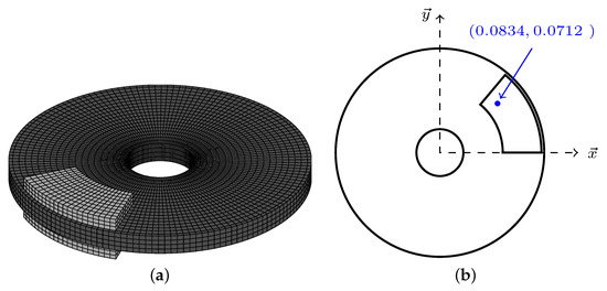
Figure 1.
Simplified brake system under study (a) Finite Element Model (b) Position of the selected point for the description of the nonlinear dynamic response.

Table 1.
Model parameters.
- The two frictional interfaces between the disc and the two pads are composed of 220 contact nodes. It should be noted that previous studies [4,5] have been performed to validate the mesh refinement on the system under study;
- The four corners of the back plate of the upper pad (pad 1) are connected to a master node which is only allowed to move in the out of plane direction;
- The inner edge of the disc (i.e., cylindrical surface in the Z direction having a radius of 0.034 m) and the back plate of the lower pad (pad 2) are clamped;
- The hydraulic pressure (2 × Pa for the present study) is directly applied on the back plate of the upper pad (pad 1);
- The nonlinearities at the friction interface between the pads and the disc are due to the cubic nonlinear terms with the the possibility of contact/no-contact states, such aswhere defines the normal reaction at the couple of matching nodes on any interface and is the relative normal displacement between one pad and the disc. and are the linear and nonlinear stiffnesses at the friction interfaces (with N·m and N·m). It should be noted that this formulation has been validated by experimental compression tests [23,24];
- The normal reaction forces on each pad is classically modeled by ;
- The friction forces are determined with a classical Coulomb’s law and the friction coefficient at the different contacts between the two pads and the disc masses is supposed to be constant and equal to . It should be noted that the same coefficient of friction is used for the two frictional interfaces for the sake of simplicity;
- The tangential friction forces are related to the normal reaction forces by where defines the local orthoradial in-plane direction (i.e., );
- The structured mesh uses hexahedrons with linear interpolation. The spatial discretization in the Z direction (i.e., thickness of the disc and pads) is of four nodes for the disc and three nodes for each pad. The spatial discretization on the circumference of the disc is of 150 nodes. The full FEM model has a total of around 50,000 degrees of freedom.
Additionally, two reduction techniques (i.e., the Craig and Bampton technique (C&B) [25] and Double Modal Synthesis (DMS)) are used on the previous FEM system to condense the number of degrees of freedom. It is recalled that the C&B technique allows us to condense each substructure (i.e., the two pads and the disc), whereas the DMS technique condenses the remaining degrees of freedom at the two frictional interfaces. The interested reader is referred to the following previous studies for more details [20,21,22].
Finally the equations of motion for the reduced brake system are given by
where is the generalized displacements vector while the dot denotes derivative with respect to time. and correspond to the global nonlinear forces at the two interfaces (i.e., ) and the hydraulic pressure, respectively. , and are reduced mass, damping and stiffness matrices, respectively. The reduced matrices for each contribution of the FEM brake system are given by
where the subscript refers to the initial data of the problem without condensation. denotes the transpose of a matrix . defines the transfer matrix between the initial reference model and the C&B condensed model. and correspond to the left and right eigenmodes of the interface degrees of freedom. They are associated with the transition from the C&B condensed model to the final reduced model that includes both C&B and DMS reductions.
In the following section, the convergence study versus the two reduction techniques will be discussed as follows:
- The C&B technique is performed by condensing the internal degrees of freedom of each substructure (i.e., the disc and the two pads) and by keeping the physical degrees of freedom situated at the two frictional interfaces. The number of fixed interface modes is chosen so that the reduced model is valid for a given frequency range of interest (i.e., with kHz in the present case). To reach such an objective, the convergence study is performed on the control parameter , selected for each substructure: the fixed interface modes whose frequencies are less than are kept;
- The DMS technique consists in the condensation of all the degrees of freedom at the two frictional interfaces. The control parameter for the DMS reduction is set by the number of interface modes kept (denoted ).
2.2. Basic Results for the Stability Analysis and the Transient Nonlinear Dynamics
The main aim of this section is to provide some basic results concerning the stability of the brake system under study, as well as the nonlinear self-sustaining dynamic response if the system is unstable.
First of all the stability of the system can be determined by using the well-known Complex Eigenvalue Analysis (CEA). Stability is determined by considering the real part of eigenvalues for the characteristic linearized equation at the equilibrium point. If all eigenvalues have negative real parts, the system is stable. If at least one eigenvalue has a positive real part, the system is unstable. The imaginary part of the associated positive eigenvalue defines the angular frequency of the unstable mode. Table 2 summarizes numerical results concerning the stability analysis of the original or reduced FEM system versus the friction coefficient (all other parameters are considered fixed). For , the system is stable. For , the system has one instability, and for , the system has two instabilities with the appearance of a second coalescence pattern. It should be noted that the convergence study versus the stability analysis for the C&B and DMS reductions is out of the scope of the present paper. The interested reader is referred to the previous studies [20,21] for more details.
Table 2.
Stability analysis of the system versus the friction coefficient.
Then, Figure 2 illustrates the nonlinear self-sustaining dynamic response of the system and the spectrograms for at the frictional interface by using the full original model. The position of the selected point is given in Figure 1. For t = [0; 0.2] s, a classical exponential increase in the solution from the perturbed equilibrium is shown. Then a transient nonlinear behavior appears (for t = [0.2; 0.5] s) with the predominant presence of the second unstable mode and its harmonic . Finally a stabilized regime is obtained for t > 0.8 s with the appearance of the first unstable mode and harmonic components , and . The presence of the harmonic combination for t = [0.4; 0.6] s is also observed, which illustrates the potential complex transient nonlinear behavior of the brake system under study. As a reminder, the appearance of such nonlinear components illustrates the limitations of the stability analysis that may lead to an underestimation of the frequency components during squeal events.
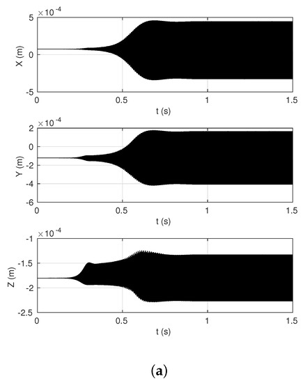
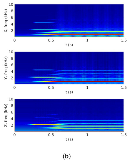
Figure 2.
Transient nonlinear behavior of the system for μ=0.8 (a) time responses and (b) spectrograms.
2.3. Prediction of Squeal Noise Based on Acoustic Radiation
One of the most important goals in the field of friction-induced vibration is to be able to predict not only the stability and transient nonlinear behavior of the system but also the acoustic noise during brake squeal. To meet this goal, one of the most popular approaches for modeling the acoustic problem is based on the Boundary Element Method (BEM). The BEM can be decomposed into two main steps: first the surface sound pressure calculation which depends on the surface normal velocity field , and secondly the estimation of the free space sound pressure by calculating the surface sound pressure. The associated equation corresponding to the second step is defined by:
where corresponds to the sound pressure over the system skin (denoted by ) and defines the pulsation. The scalar is in [0; 1] depending on the location of the calculated pressure : = 1 in the radiation space and on boundaries). denotes the outside normal of . is the sound pressure in the free space and and are the BEM matrices (for more details see [26,27]). It is important to note that the term is a known value since it is directly linked to the surface normal velocity , which is an output value of the structural calculation.
The previous fields depend on the pulsation . So, the BEM has to be applied for each harmonic component of the nonlinear response of the brake system in order to estimate the acoustic radiation. For the present study, the multifrequency acoustic calculation method [5], that allows us to calculate the global sound pressure ( in the free space and over the mesh) by superposition of the BEM results for each frequency, is applied to estimate the noise levels over the mesh and at every point in free space. One of the main advantage of this methodology is that only the predominant contributions are used for the global estimation of the acoustic radiation. The pressure level in dB can be calculated, such as , where Pa and denote the conjugated elements. For the system under study, it should be mentioned that we propose the boundary element model that is composed of the upper or inner part of the brake system skin for the calculation of the acoustic radiation. Figure 3 and Figure 4 illustrate the classical converged acoustic results for the steady state vibration regime of the brake system on three horizontal planes and two vertical planes, respectively. It should be noted that the center of the disc is located at position (0,0,0).
Figure 3.
Acoustic patterns in dB for the steady state vibration regime (for t > 1 s) on different horizontal planes at 0.25 m, 0.75 m and 1.25 m.
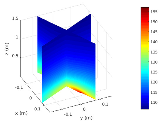
Figure 4.
Acoustic patterns in dB for the steady state vibration regime (for t > 1 s) on two vertical planes.
3. Approximation of the Acoustic Radiation Based on Multiresolution Signal Decomposition and Convergence Study of Reduced Basis
In this section we propose a tool allowing us to compare the acoustic fields calculated by the reference solution and different reduced models. A strategy based on a decomposition of acoustic patterns and a multi-resolution representation for analyzing information content of acoustic patterns is developed. This method makes it possible to analyze details of acoustic pattern on different observation scales ranging from the pixel to the size of the complete pattern. For the present study, this will allow us to have a notion of convergence with respect to different patterns of the acoustic field emitted during squeal noise.
First, a reminder of the notion of the windowed Fourier Transform as well as wavelets and their extension to the two-dimensional case is proposed. Then the proposed approach based on the multiresolution signal decomposition with the wavelet representation and the decomposition algorithm proposed by Mallat [28,29] are developed. The use of such an approach for a convergence study of squeal noise is discussed and some convergence criteria are proposed for the analysis of acoustic fields. Finally, the efficiency of the proposed strategy is undertaken based on numerical results.
3.1. On the Use of Windowed Fourier Transform
Signal analysis is traditionally done using Fourier decompositions on a trigonometric function basis for a periodic signal, or more generally using the Fourier transform of any function as indicated in Equation (9). These methods allow for a signal of finite duration to express its frequency content. However, the Fourier transform is not adapted to non-stationary signals and to the localization of high frequencies.
In order to overcome this problem, a first idea is to perform windowed Fourier transforms on predefined signal portions in order to better identify the high frequency components. Considering the windowing function g, we can define in Equation (10) a windowed Fourier transform , centered around an observation point . The g function allows us to spatially filter the f function around an interval of interest centered on and therefore to detect the associated frequency components.
By defining and as the standard deviations associated with the functions g and , respectively, the uncertainty principle applied to the function g implies the following relation . This inequality defines the compromise to be made between spatial and frequency resolutions. Figure 5a illustrates this inequality in the 2D dimension . which only allows for the description of f around the point and for an interval . Thus cells of constant area and identical form are defined. This regular decomposition thus imposes that the discretization in frequencies of the studied problem is also regular and uniform. All the frequency intervals are therefore of the same size and they are distributed linearly, which therefore imposes a compromise between the spatial and temporal refinements of the windowing function g. In our study, the signals to be analyzed are composed of non-uniformly distributed frequencies, which makes the windowed Fourier transform unsuitable.
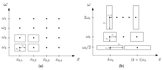
Figure 5.
Diagram of observation cells and variable mesh in the 2D dimension (a) Fourier representation (b) Wavelet representation.
3.2. Wavelet Transform and Logarithmic Observation Scales
Due to the fact that the conventional Fast Fourier Transform (FFT)-based spectral analysis method provides poor representation of signals well localized in time, time-scale signal processing tools have to be used to provide a good description of signals. Morlet [30] proposed applying the wavelet approach to analyze the vibration of systems. The wavelet analysis transforms a signal into wavelets that are well localized in both frequency and time. The wavelet transform can be expressed as
where defines the mother wavelet. s corresponds to the expansion factor: it allows the function to observe the studied signal f at a particular position . From the mother wavelet, it is possible to define a function , where the expansion factor s allows her to move the frequency of the bandpass filter of the base function and then to modify the width of the frequency band. By denoting the usual scalar product of , it is then possible to rewrite the wavelet transform as a convolution product between the function f and the wavelet , such as
Any function can thus be decomposed on the basis , such as
with with . defines a wavelet family that corresponds to an orthonormal basis of . For a given observation scale , the set of functions defines the vector subspace . Each corresponds to a multiresolution vector space sequence. It can be noted that , which reflects the fact that the successive sets of function approximations, allows for a more precise description of any function by a factor of 2. We can define the operator which approximates some function at a resolution , such as
It should be noted that is a linear operator. is not modified if we approximate it again at the resolution (i.e., is a projection operator on a particular vector space ).
Then, it is possible to extract the difference of information between the approximation of a function at the two resolutions and . The discrete detail signal is given by
which represents the difference of information between the resolutions and . It should be noted that the resolutions and of the function are, respectively, equal to its orthogonal projection on and . So the discrete detail signal is given by the orthogonal projection of the original signal on the orthogonal complement of in , such as .
Mallat [28,29] proposes an iterative algorithm allowing us to calculate the signal at the lower resolution (i.e., ) as well as the information between the resolutions and (i.e., ) from a signal . From an original signal, measured at a resolution of 1, it is then possible to obtain its decomposition up to an order . This set of discrete signal sets is called an orthogonal wavelet representation and it represents the signal at a coarse resolution as well as all associated detail signals at the intermediate resolutions with .
The advantage of this wavelet decomposition is that the change of scale is here logarithmic, whereas it was linear for the windowed Fourier transform. This affects the shape of the observation cells in the space . Assuming that the function has zero mean, a standard deviation and its Fourier transform centered around with a standard deviation of , the cells described by different wavelets of the form cover the area , as illustrated in Figure 5b. It is clearly shown that when the observation scale s is small, the spatial resolution is coarse, while the frequency resolution is fine. When the observation scale s increases, the spatial resolution becomes finer but the frequency domain also increases in size. The spatial resolution is therefore not the same from one scale to another. It is perfectly suited to the study of non-stationary signals composed of several frequency components by making it possible to locate specific frequency components in the signal.
3.3. Extension of the Orthogonal Wavelet Representation to the Two-Dimensional Case
In this section, we briefly develop the two-dimensional case for acoustic radiation images corresponding to squeal noise. More details can be found in [28,29].
We focus on the extension for a function in for which the scalar product is given by
For multiresolution approximations, each vector space can be decomposed as a tensor product of two identical sub-spaces of , such as , . Then the scaling function whose dilatation and translation given an orthonormal basis of each space , can be defined by , where is the one-dimensional scaling function of the multiresolution approximation . The, the orthogonal basis of can be defined by
It should be noted that relation between the multiresolution approximation and can be easily defined by [28,29]
where defines the orthogonal complement of in as previously discussed in Section 3.2. As previously discussed in Section 3.2 for the one-dimensional case, the detail signal at the resolution is still equal to the orthogonal projection of the signal on the orthogonal complement of . Mallat [28,29] demonstrated that this orthogonal complement can be defined by scaling and translating the three following wavelets functions
where and are, respectively, the one-dimensional scaling function of the multiresolution approximation and .
Then, it is possible to define the operator , which approximates the function at a given resolution , such as
The difference of information between and can also by defined by the three following detailed images (in the three orthonormal directions)
Finally, it can be concluded that an two-dimensional image is completely represented by the discrete images defined by the decomposition
where J corresponds to the number of iterations for the decomposition of the original image. Figure 6 illustrates the decomposition process and the disposition of , , and for three iterations.
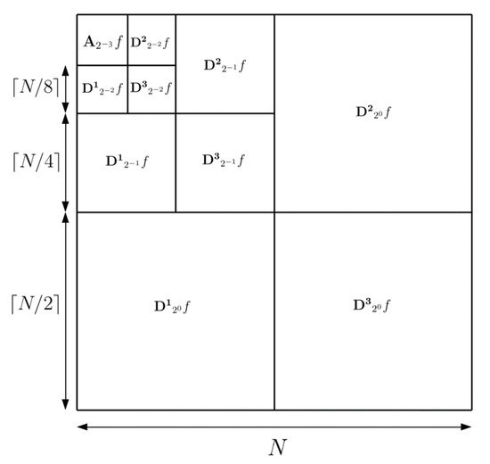
Figure 6.
Illustration of the 2D wavelet decomposition of a pattern of size N for three iterations, according to Mallat’s algorithm.
3.4. Application for Squeal Noise and Convergence Results
3.4.1. Preamble: On the Use of the Multiresolution Signal Decompostion for Squeal Noise and Definition of Convergence Criteria
The acoustic results for the prediction of squeal noise can be defined by matrices of coefficients representing the acoustic intensity on a discretized two-dimensional space (see for example the three images in 2D-dimension from Figure 3). These images are bounded patterns with a given resolution. There is therefore a maximum resolution beyond which it is no longer possible to extract detail from the signal. This resolution is linked to the mesh of the surface. Therefore, it defines the starting resolution of the decomposition algorithm.
Since the acoustic observation surface is bounded, there is a minimum observation scale, beyond which the decomposition algorithm reaches a resolution which is that of the size of the surface itself. Assuming that the image of acoustic radiation is given by a matrix of size with , this minimum resolution is equal to where sets rounding to the next higher unit. In this case, the two-dimensional image is completely represented by the discrete images with the decomposition given in Equation (24). The matrices given in Equations (20)–(23) that correspond to the first iterations of j are those which analyze details at a fine resolution. So they can be associated with a small wavelength which characterizes the fine details of the pattern. On the contrary, the matrices associated with a larger j are those that reflect the fluctuations at high wavelength, characterizing the overall appearance of the two-dimensional studied image.
So, it is possible to quantify the differences in the representation of the acoustic fields for different reduced models by analyzing and comparing details of a pattern for different C&B and DMS reductions, and this is for different observation scales ranging from the pixel to the size of the complete acoustic pattern. In order to quantify the quality of the convergence based on C&B or DMS reductions for the two-dimensional acoustic radiation, a first criterion based on the relative error between a signal f and the reference signal is proposed, such as
with
where defines the Frobenius norm. It should be noted that one of the major advantages of this criterion is that it makes it possible to have an appreciation of the quality of the convergence for different scales of observations (i.e., for each ) on the complete 2D image of the estimated acoustic field.
Additionally, a global criterion , allowing us to obtain an evaluation of the overall error between a pattern f and the reference pattern , is proposed, such as
Note that the two proposed criteria, and , are complementary: the first allows us to have a detailed analysis with respect to several scales of representation and thus to study the relevance of a reduced model for an approximation of the acoustic radiation at a given resolution, while the second corresponds to a global vision and allows us to estimate the relevance of a basis reduction for an accumulation of representation scales.
3.4.2. Application and Numerical Results
Figure 7 and Figure 8 give the evolution of at , depending of the size of the C&B basis as well as DMS basis for the acoustic patterns during the steady state vibration regime on the three horizontal planes (at 0.25 m, 0.75 m and 1.25 m, as previously defined in Figure 3) and the two vertical planes (as previously defined in Figure 4), respectively. It should be noted that each size of the C&B reduction (i.e., the value of ) and each size of the DMS reduction (the value of ) is associated with the color bar and the definitions of the color bar are explained in the legend of Figure 7 and Figure 8.
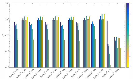
Figure 7.
Values of for —horizontal planes (definition of the color bar for “Scale 2—CB”: 1 , 2 , 3 , 4 , 5 ; definition of the color bar for “Scale 2—DMS”: 1 , 2 , 3 , 4 , 5 , 6 , 7 .
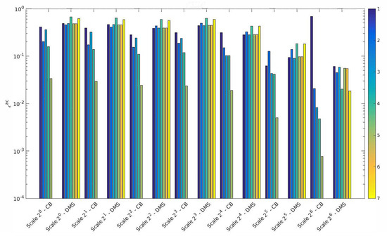
Figure 8.
Values of for —vertical planes. Definition of the color bar for “Scale 2—CB”: 1 , 2 , 3 , 4 , 5 ; definition of color bar for “Scale 2—DMS”: 1 , 2 , 3 , 4 , 5 , 6 , 7 .
First of all, it is clearly shown that the C&B reduction technique converges very well—increasing and decreasing for each scale of observation (see more specifically bars for the legends “Scale 2—CB” for j = 1 to 6). Of course, this conclusion is also clearly illustrated by showing the evolution of , as illustrated in Figure 9. It can also be observed that the convergence results are very similar for the two cases (i.e., acoustic patterns on the horizontal and vertical planes). These results indicate that increasing (i.e., the size of the C&B reduction) allows us to enhance the visualization (i.e., image) of the acoustic radiation and therefore the prediction of the squeal noise. In order to illustrate this fact, Figure 10 gives the acoustic patterns on one chosen horizontal plane (at the distance of 0.75 m in the direction z, the second horizontal plane in Figure 3) for the reference model (denoted “Ref.”, first line of Figure 10) and two chosen C&B reductions (with and in the second and third lines of Figure 10, respectively). The result obtained for is very similar to the reference both in form and in acoustic level, while the results for are worse with an overestimation of the acoustic intensity.
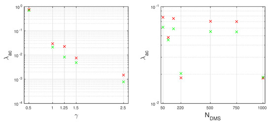
Figure 9.
Values of at for horizontal planes (red) and vertical planes (green).
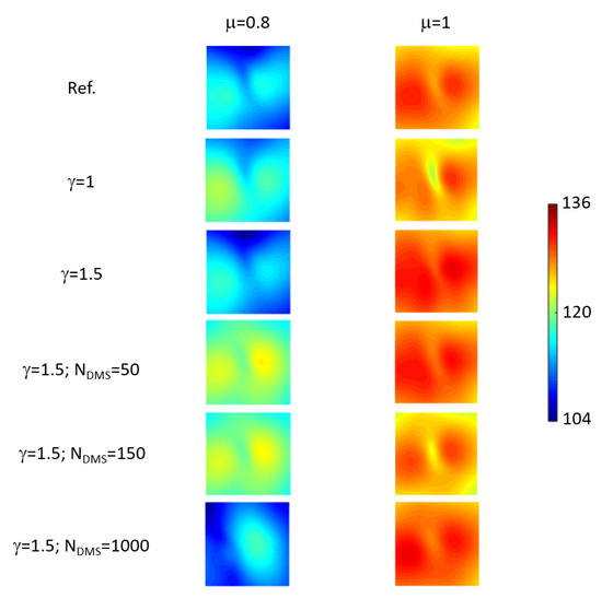
Figure 10.
Acoustic patterns on the horizontal plane at the distance of 0.75 m in the direction Z for different C&B and DMS reductions, scale in dB.
Then, in order to analyze only the effects of the DMS size, the reference is chosen as the numerical result of the C&B reduction technique with (i.e., this choice avoids introducing cumulative errors from the two successive C&B and DMS reductions in the value of ). It should be noted that the reduced system comprises 2885 degrees of freedom, divided into 2640 degrees of freedom at the interfaces (i.e., spatial physical degrees of freedom), plus 245 generalized degrees of freedom corresponding to the modes with fixed interfaces (103 generalized degrees of freedom (dof) for the disc, 111 generalized dof for the upper pad and 31 generalized dof for the lower pad). Analyzing the convergence of the DMS basis in Figure 7 and Figure 8 (see more specifically bars for the legends “Scale 2—DMS” for j = 1 to 6), it is observed that increasing the number of interface modes (i.e., ) does not significantly decrease . In fact this result demonstrates that considering few complex eigenmodes (i.e., ) seems to be enough to provide a satisfactory approximation of the radiated fields at different resolutions. Results for reinforce this conclusion with a value of inferior of 8 × 10, whatever the size of the tested DMS basis. Note that, in the present case, convergence results for and are provided by applying, beforehand, the C&B reduction technique with . Figure 10 also gives the visualization of the acoustic radiation on the horizontal plane at the distance of 0.75 m for three DMS reductions (, and , the last three lines of Figure 10), to be compared with (i.e., the third line of Figure 10).
In order to further illustrate the relevance of the proposed methodology, numerical simulations are carried out to estimate the radiated acoustic field for . Figure 11 gives the evolution of for different C&B and DMS bases. Moreover Figure 10 gives the associated acoustic patterns for the reference model, two C&B bases and three DMS reductions (see the second column of Figure 10). All the results are in agreement with the discussion made previously for : increasing (i.e., the size of C&B basis) increases the quality of the estimation of the approximated acoustic noise, whereas increasing the number of complex interface modes (i.e., ) does not significantly improve the image quality of the radiated field. It is also interesting to note that the results presented for the two cases ( and ) give very different radiated field levels as illustrated in Figure 10 (see and compare the first and second columns). All these results illustrate the fact that the two proposed criteria and give an error between a pattern f and the reference pattern which makes it possible to judge the quality of the approximation to the acoustic field. Some additional investigations should be done in the future to provide a robust strategy to efficiently decide on the sizes of the C&B and DMS bases that are relevant to give a adequate spatial representation of the radiated field based on the two criteria and .
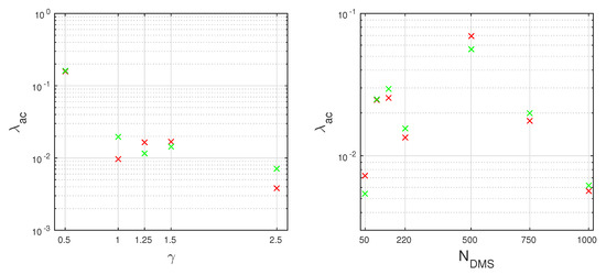
Figure 11.
Values of at for horizontal planes (red) and vertical planes (green).
Finally, some additional theoretical comments can be added for a better understanding of the convergence of the DMS basis. From a physical point of view, a succession of contact/non-contact states can occur during self-excited vibrations. However, a DMS basis is initially calculated for a specific equilibrium point (with the definition of the complex interfaces modes, see [21] for more details) and for each friction coefficient (unlike the Craig and Bampton reduction). Even if it is possible to globally reproduce the nonlinear vibration behavior as well as the squeal noise of the brake system with a small size of DMS basis, increasing the size of DMS basis does not imply a significant improvement in the prediction of the squeal noise due to the fact that some physical complex states at the frictional interface can not be exactly described (but only approximated). Moreover it has been observed that a DMS reduction with leads to bad results. This is a classic result of the DMS method which requires to retain a certain number of interface modes to start getting relevant results.
4. Conclusions
This study proposes to evaluate the efficiency of the Double Modal Synthesis (DMS) method that involves the use of a classical Craig and Bampton modal reduction on each substructure considering the interface surfaces associated to condensation at the frictional interface based on complex modes, for the prediction of squeal noise and the visualization of the resulting acoustic fields on different horizontal and vertical planes.
To reach such an objective, two criteria, and , and a methodology based on the multiresolution signal decomposition of acoustic radiation with wavelet representation, have been proposed. The proposed strategy allows us to define which reduced model is able to properly approximate various images of acoustic patterns during squeal events.
All the numerical results indicated that a reduced basis built with the DMS technique is able to reproduce the essential physical phenomena present during friction and self-excited vibration and so to provide a good approximation of the acoustic patterns and 2D visualization of squeal noise.
Author Contributions
Conceptualization, G.C., J.-J.S. and S.B.; Data curation, G.C.; Investigation, G.C., J.-J.S. and S.B.; Methodology, G.C., J.-J.S. and S.B.; Validation, J.-J.S. and S.B.; Visualization, G.C.; Writing—original draft, J.-J.S.; Writing—review and editing, J.-J.S. and S.B.; All authors have read and agreed to the published version of the manuscript.
Funding
This research received no external funding.
Acknowledgments
J.-J.S. acknowledges the support of the Institut Universitaire de France.
Conflicts of Interest
The authors declare no conflict of interest.
References
- Oberst, S.; Lai, J.; Marburg, S. Guidelines for numerical vibration and acoustic analysis of disc brake squeal using simple models of brake systems. J. Sound Vib. 2013, 332, 2284–2299. [Google Scholar] [CrossRef]
- Oberst, S.; Lai, J. Squeal noise in simple numerical brake models. J. Sound Vib. 2015, 352, 129–141. [Google Scholar] [CrossRef]
- Lee, H.; Singh, R. Determination of sound radiation form a simplified disk-brake rotor by a semi-analytical method. Noise Control Eng. J. 2004, 52, 225–239. [Google Scholar] [CrossRef]
- Soobbarayen, K.; Besset, S.; Sinou, J.-J. A simplified approach for the calculation of acoustic emission in the case of friction-induced noise and vibration. Mech. Syst. Signal Process. 2015, 50–51, 732–756. [Google Scholar] [CrossRef]
- Soobbarayen, K.; Besset, S.; Sinou, J.-J. Noise and vibration for a self-excited mechanical system with friction. Appl. Acoust. 2013, 74, 1191–1204. [Google Scholar] [CrossRef]
- Soobbarayen, K.; Sinou, J.-J.; Besset, S. Numerical study of friction-induced instability and acoustic radiation—Effect of ramp loading on the squeal propensity for a simplified brake model. J. Sound Vib. 2014, 333, 5475–5493. [Google Scholar] [CrossRef]
- Sinou, J.-J.; Lenoir, D.; Besset, S.; Gillot, F. Squeal analysis based on the laboratory experimental bench Friction-Induced Vibration and Noise at Ecole Centrale de Lyon. Mech. Syst. Signal Process. 2018, 119, 561–588. [Google Scholar] [CrossRef]
- Lenoir, D.; Besset, S.; Sinou, J.-J. Transient vibro-acoustic analysis of squeal events based on the experimental bench FIVEECL. Appl. Acoust. 2020, 165, 107286. [Google Scholar] [CrossRef]
- Akay, A. Acoustics of friction. J. Acoust. Soc. Am. 2002, 11, 1525–1548. [Google Scholar] [CrossRef]
- Crolla, D.; Lang, A. Brake noise and vibration—State of the art. Tribol. Ser. 1991, 18, 165–174. [Google Scholar]
- Papinniemi, A.; Lai, J.; Zhao, J.; Loader, L. Brake squeal: A literature review. Appl. Acoust. 2002, 63, 391–400. [Google Scholar] [CrossRef]
- Kinkaid, N.; O’Reilly, O.; Papadopoulos, P. Automotive disc brake squeal. J. Sound Vib. 2003, 267, 105–166. [Google Scholar] [CrossRef]
- Ibrahim, R. Friction-induced vibration, chatter, squeal, and chaos—Part II: Dynamics and modeling. Appl. Mech. Rev. 1994, 47, 227–253. [Google Scholar] [CrossRef]
- Ibrahim, R. Friction-induced vibration, chatter, squeal and chaos Part 1: Mechanics of contact and friction. Appl. Mech. Rev. 1994, 47, 209–226. [Google Scholar] [CrossRef]
- Ouyang, H.; Nack, W.; Yuan, Y.; Chen, F. Numerical analysis of automotive disc brake squeal: A review. Int. J. Veh. Noise Vib. 2005, 1, 207–231. [Google Scholar] [CrossRef]
- Vermot des Roches, G. Frequency and Time Simulation of Squeal Instabilities. Application to the Design of Industrial Automotive Brakes. Ph.D. Thesis, École centrale Paris, Paris, France, 2011. [Google Scholar]
- Lai, V.V.; Chiello, O.; Brunel, J.F.; Dufrenoy, P. Full finite element models and reduction strategies for the simulation of friction-induced vibrations of rolling contact systems. J. Sound Vib. 2019, 444, 197–215. [Google Scholar] [CrossRef]
- Brizard, D.; Chiello, O.; Sinou, J.-J.; Lorang, X. Performances of some reduced bases for the stability analysis of a disc/pads system in sliding contact. J. Sound Vib. 2011, 330, 703–720. [Google Scholar] [CrossRef]
- Loyer, A.; Sinou, J.-J.; Chiello, O.; Lorang, X. Study of nonlinear behaviors and modal reductions for friction destabilized systems. Application to an elastic layer. J. Sound Vib. 2012, 331, 1011–1041. [Google Scholar] [CrossRef][Green Version]
- Monteil, M.; Besset, S.; Sinou, J.-J. A double modal synthesis approach for brake squeal prediction. Mech. Syst. Signal Process. 2016, 70–71, 1073–1084. [Google Scholar] [CrossRef]
- Besset, S.; Sinou, J.-J. Modal reduction of brake squeal systems using complex interface modes. Mech. Syst. Signal Process. 2017, 85, 896–911. [Google Scholar] [CrossRef]
- Sinou, J.-J.; Besset, S. Simulation of transient nonlinear friction-induced vibrations using complex interfaces modes: Application to the prediction of squeal events. Shock Vib. 2017. [Google Scholar] [CrossRef]
- Sinou, J.-J.; Coudeyras, N.; Nacivet, S. Study of the nonlinear stationary dynamic of single and multi instabilities for disc brake squeal. Int. J. Veh. Des. 2008, 1–2, 207–222. [Google Scholar]
- Sinou, J.-J. Transient non-linear dynamic analysis of automotive disc brake squeal – On the need to consider both stability and non-linear analysis. Mech. Res. Commun. 2010, 37, 96–105. [Google Scholar] [CrossRef]
- Craig, R.; Bampton, M. Coupling of substructures for dynamic analyses. AIAA J. 1968, 6, 1313–1319. [Google Scholar] [CrossRef]
- Marburg, S.; Nolte, B. Computational Acoustics of Noise Propagation in Fluids; Springer: Berlin/Heidelberg, Germany, 2008. [Google Scholar]
- Bonnet, M. Boundary Integral Equation Methods for Solids and Fluids; John Wiley & Son Ltd.: Chichester, UK, 1999. [Google Scholar]
- Mallat, S. A Theory for Multiresolution Signal Decomposition: The wavelet representation. IEEE Trans. Pattern Anal. Mach. Intell. 1989, 11, 674–693. [Google Scholar] [CrossRef]
- Mallat, S. Multifrequency channel decompositions of images and wavelet models. IEEE Trans. Acoust. Speech Signal Process. 1989, 37, 2091–2110. [Google Scholar] [CrossRef]
- Morlet, J. Sampling Theory and Wave Propagation; NATO ASI Series; Springer: Heidelberg, Germany, 1983; pp. 233–261. [Google Scholar]


Publisher’s Note: MDPI stays neutral with regard to jurisdictional claims in published maps and institutional affiliations. |
© 2020 by the authors. Licensee MDPI, Basel, Switzerland. This article is an open access article distributed under the terms and conditions of the Creative Commons Attribution (CC BY) license (http://creativecommons.org/licenses/by/4.0/).