Article

Preliminary Investigation of the Performance of an Engine Equipped with an Advanced Axial Turbocharger Turbine

by
Gregory Guarda
1,
Apostolos Pesyridis
1,2,* and
Ashish Alex Sam
1,3
1
Department of Mechanical and Aerospace Engineering, Brunel University London, London UB8 3PH, UK
2
Alasala Colleges, King Fahad Bin Abdulaziz Rd., Dammam 31483, Saudi Arabia
3
CO2 Research and Green Technologies Centre, Vellore Institute of Technology (VIT), Vellore 632014, Tamil Nadu, India
*
Author to whom correspondence should be addressed.
Appl. Sci. 2020, 10(21), 7452; https://doi.org/10.3390/app10217452
Submission received: 24 July 2020 / Revised: 25 September 2020 / Accepted: 22 October 2020 / Published: 23 October 2020

Abstract

:
Stringent emission regulations and increased demand for improved fuel economy have called for advanced turbo technologies in automotive engines. The use of turbochargers on smaller engines is one such concept, but they are limited by a time delay in reaching the required boost during transient operation. The amount of turbocharger lag plays a key role in the driver’s perceived quality of a passenger vehicle’s engine response. This paper investigates an alternative method to the conventional design of a turbocharger turbine to improve the transient response of a passenger vehicle. The investigation utilises the Ford Eco-Boost 1.6 L petrol engine, an established production engine, equipped with a turbocharger of similar performance to the GT1548 produced by Honeywell. The commercially available Ricardo WAVE was used to model the engine. Comparing the steady-state performance showed that the axial turbine provides higher efficiencies at all operating conditions of an engine. The transient case demonstrated an improved transient response at all operating conditions of the engine. The study concluded that, by designing a similar sized axial turbine, the mass moment of inertia can be reduced by 12.64% and transient response can be improved on average by 11.76%, with a maximum of 21.05% improvement. This study provides encouragement for the wider application of this turbine type to vehicles operating on dynamic driving cycles such as passenger vehicles, light commercial vehicles, and certain off-road applications.

1. Introduction

During recent years, emissions legislation for automotive manufacturing has become more restrictive, requiring much more advanced exhaust after treatment systems. This requirement puts heavy demand on manufacturers to provide unique solutions to meet these targets. The downsizing of engines provides an alternative solution to reducing the emission levels produced in passenger cars as well as to improving fuel consumption. Spark ignition engines can have an expected 40% smaller displacement along with 25% improved combustion performance by implementing a turbocharger [1]. The use of smaller engines, operating with less fuel than that of their larger counterparts, directly reduces the amount of emissions produced, which also reduces fuel consumption.
With the increase in turbocharged passenger vehicles, driver demand for reduced “turbo lag” will likely follow or, from the driver’s point of view, the delay in throttle response. Turbo lag is a measure of the time delay for a turbo spinning at low speed, where no boost is produced, to be brought up to the speed, where it can function effectively [2]. The reduction of turbo lag can be associated with the design of the turbine component of the turbocharger, used to recover energy in the exhaust gases to mechanical energy. Turbo lag is mostly apparent at low engine speeds, where the exhaust mass flow rate is not sufficient to provide enough energy to drive the turbine. Many methods have been suggested and tested to reduce turbo lag, but fundamentally, the most important is reducing the mass moment of inertia. An alternative method suggested by the Ford Motor Company (Dearborn, MI, USA) was the implementation of an axial inflow turbine to improve transient response [3].
Conventionally, turbocharger turbines employed in the automotive industry are radial inflow, whereby the exhaust gas enters the rotor radially and leaves axially. The axial turbine is different, in that the exhaust gases are axially guided by stationary guide vanes (stators) onto the rotor. Thus, the flow through the rotor is predominantly in axial and tangential directions and there is no radial change in the flow across the rotor. The benefit of this method over its conventional counterpart is that it typically, at the same diameter, provides a higher total-to-static efficiency and thus produces more power for the same flow conditions. This means that the axial rotor diameter can be reduced to produce the same power as its radial counterpart, thus reducing its mass and its inertia [4].
Even with lower inertia, like its radial counterpart, the axial turbine is still limited by turbo-lag, which is more evident at lower engine speeds and load conditions. Variable geometry turbine (VGT) technology is used to improve the performance of turbines at lower flow rates as well as higher flow rates by interacting with the flow to change the velocity and flow angles to achieve better turbine performance. The literature also reports the use of mixed flow turbines in turbocharger applications [5,6]. The use of mixed flow turbines reduces inertia, and they also provide a flat efficiency characteristic, enhancing the performance at lower blade speed ratios.
This paper however carries forward the analysis of an axial turbine concept carried out by Pesyridis et al. [7,8]. The objective of this paper is to analyse the transient response of the turbocharger system using the axial turbine and to compare it with a conventional radial turbine. By necessity, certain assumptions are embedded (see Section 3) and a detailed scaling method is presented (in Section 2.2) in converting the turbine for appropriate use for this particular engine application. The methodologies and results presented below are extensive, using real-world engine data, but did not intend to be applicable to the specific production engine. The methodology was based around the idea of proximity to the performance of a popular, mass production engine, with the ultimate goal being detailed comparison and discussion of the merits of the presented axial turbine versus the baseline radial turbine in current use.

2. Literature Review

2.1. Axial Turbines for Turbocharging

Honeywell Turbo Technologies (HTT) presented a report detailing a breakthrough in the development of an axial turbine for improved transient response with their DualBoostTM turbocharger. The results demonstrated a reduction in turbo lag of 25% by reducing the mass moment of inertia by 50% [9]. Figure 1 shows the comparison of the total to static efficiency between the newly developed DualBoostTM turbine and the baseline radial. The figure demonstrates that the axial turbine is more effective under low-velocity (blade tip to absolute gas flow velocity) ratios in recovering energy from exhaust gas. However, the theoretical maximum efficiency of the axial turbine is lower than that of the radial turbine.
This technology, however, is not relatively new. Ford Motor Company (Dearborn, MI, USA) conducted a testing in 1985 to assess the performance of an axial turbine when compared to a radial turbine on a 2.3-L engine under transient conditions. The study identified that the axial turbine could produce the same “flow and peak efficiency characteristics” as its radial counterpart at different engine speeds but with a lower inertia. The results of the study demonstrated a 25% to 40% improvement on the transient response of the turbocharger, with just under 50% mass moment of inertia reduction. This provides a target for the design considered in the present work to achieve at least a 25% improvement in transient response [3].
Despite the discussed advantages in the implementation of the axial turbines, there are few challenges associated with it. Axial turbines are predominantly found in aerospace and large power generation applications. For automotive turbochargers, as the power range is in kilowatts, blade height for axial turbines is comparatively smaller than radial turbines and would result in disproportionate increase in leakage flow effects. Therefore, a key challenge is the corresponding decrease in efficiency with a decrease in size. This calls for finer manufacturing tolerances and, in turn, makes the employment of axial turbines for turbocharger applications more costly [10]. Hence, increases in aerodynamic efficiency are of paramount importance in the successful employment of such designs. In addition, for the successful implementation of an axial turbine design, a detailed flow field and rotor dynamic analysis of the turbine needs to be performed followed by transient performance testing of the turbocharger and engine. This type of research is ongoing but outside the scope of this paper.

2.2. Turbocharging Map Scaling

Matching a turbocharger map to any given engine model is a difficult task to accomplish; several different methods throughout literature have been attempted. However, all methods start with the same fundamental principle of scaling the map in terms of dimensionless coefficients. By using this method, a map is obtained that is representative of a family of turbochargers of similar performances but of different operating conditions and sizes. For turbomachinery in the gas turbine industry, the following scaling law relationship Equation (1) is used to define the pressure ratio as a function of rotor tip Mach number, the mass flow coefficient, the Reynolds number, and the Mach number based on inlet conditions [11].
P d P u = f N T C   D R T u ,   m ˙ R T u P u D 2 , R e ,   M n
Equation (1) shows the pressure ratio for a compression process. For a turbine, it would be for the expansion process which would be the inverse of the left-hand side of Equation (1), but the right-hand side stays the same. The above equation allows for the ability to treat a tested turbocharger performance as a black box system, and similar pressure ratios can be obtained for compressors and turbines of the same family by keeping these parameters constant at each point. Thus, this assumption leads to the first stage used in most literature to scale maps to their dimensionless coefficients, giving a generic map that will govern the family. This is extremely useful when designing new equipment, as it is far easier and quicker to simply scale a map theoretically to test turbomachinery, at various diameters, than to manufacture and test.
The laws can yield comparable results for differently sized turbomachinery; however, an exact match between the similar turbomachinery cannot be achieved [12]. Therefore, to simplify the scaling of turbomachinery, it can be assumed for small scaling factors of diameter that the Reynolds number can be free to vary and that the gas-specific properties of the flow are constant [13]. This assumption has also been used in an alternative method for scaling using the polytropic infinitesimal stage [14]. Therefore, when scaling, Equation (1) can be further reduced to Equation (2).
P d P u = f N T C   D T u ,   m ˙ T u P u D 2
Equation (2) along with the black-box treatment of the turbomachinery can be better put into context by looking at a performance map shown below in Figure 2.
Even with the scaling laws simplified, matching a turbocharger to an engine is a far more difficult task in itself, as the turbomachinery diameter is not chosen but needs to be obtained to provide the desired performance, and this task needs to be accomplished simultaneously for both compressor and turbine. Bell et al. [15] showed good results for scaling process by first identifying the compressor diameter and the torque required from the turbine to reach the necessary boost, yielding good turbocharger performance results at various engine sizes. However, the author does not show whether the results were matched to specific engine performances. Nevertheless, the Ricardo WAVE balances the turbocharger shaft speed using a torque balance equation, meaning this method is viable [16].
When scaling for pressure ratios, the results shown have a good correlation between differently sized turbomachinery. However, most methods investigated have not considered scaling the efficiency, which leads to the questions, should the efficiency be scaled, or is it acceptable to assume the change as negligible to the final results? The efficiency can be established as a function of the corrected shaft speed and the pressure ratio as shown in Equation (3) [15].
Ƞ i s e n = f N c o r r ,   P u P d
Based on a previous analysis, if the pressure ratio is not changed during the scaling process, then how much the function is dependent on the corrected shaft speed should be considered. In theory, with only a small change to the turbomachinery diameter based on Equation (2), only a small change to the corrected shaft speed would be calculated; thus, dependent on the level of influence this parameter has, it could be assumed that the impact to the efficiency is negligible. Comparing this assumption with Figure 2, it is clear that a significant change to the corrected shaft speed would be needed to affect the efficiency results. An analysis by Ernst et al. [12] demonstrated that “for small trim variations (4%) the changes in pressure ratio and efficiency are negligible” and therefore scaling for efficiency should only be considered for large variations in trim (24%).

3. Methodology

The present study involves the analysis of an axial turbine design developed by Pesyridis et al. [7,8]. Preliminary design and optimization of the developed axial turbine are reported in the same literature [7,8]. Ford Eco Boost 1.6 L petrol engine with a Garrett turbocharger was chosen for the analysis. The selection procedure following the Garrett manual observed that the GT1548 was best suited for the Ford Ecoboost engine and was thus opted for further study.
The study includes the following:
(i)
Development of a correlated engine model by scaling the original GT1548 turbocharger test results to match the operating performances of the engine model to Ford Eco-Boost 1.6 L petrol engine data provided by earlier works;
(ii)
Obtainment of baseline steady-state performance results of the engine model with the scaled radial turbine implemented;
(iii)
Development of a transient model within the Ricardo WAVE to compare the turbo lag between the baseline and the new designs;
(iv)
Obtainment of performance maps to be used for implementation in all engine models to provide comparative steady-state results between designs;
(v)
Conduction of inertia testing to obtain an estimated mass moment of the GT1548 turbocharger and to then scale it to the diameters used to match the turbocharger to the engine; and
(vi)
Obtainment of all transient turbocharger data to compare the times to reach maximum shaft speed and manifold pressure against the baseline radial turbine

Transient One-Dimensional Engine Modelling

The chosen engine modelling software for this study is Ricardo WAVE. Within WAVE, there are two methods for performing a transient simulation. The first is built into WAVE and requires the implementation of a control system; the other requires exporting the model using WAVE RT to combine the model within Simulink. The first method was chosen for the present study as it is far less complex to set up as well as reduces the need for debugging to one software.
With the transient modelling, it is important that the moment of inertia is calculated correctly, taking into consideration all components of the system. Otherwise, the results could be inaccurate and will yield only theoretical results. Mishra and Saad [17] indicated a 68% transient response improvement using an electrically assisted compressor. This was achieved without including a moment of inertia for the electrical motor system by applying the assisted torque directly. Similar to this analysis, Gilkes et al. [18] investigated an air injection assist in a turbocharged 2-L diesel engine, in which the simulation (WAVE RT) suggested an excess of 15 s for the compressor to reach the required manifold pressure. Therefore, care should be taken when analysing the results to ensure they are realistic by comparing to real test data reported in the literature.
Real test data from the Ford Motor Company (Dearborn, MI, USA) report indicated that, for the 2.3 L engine, the time to reach the desired shaft speed was approximately 2 s at most tested conditions and, for HTT and the DualBoostTM, took no longer than 3 s [3,9]. This range is also concurred by results obtained by Eriksson et al. [19] from an engine model that had been fully validated with engine test data that estimated around 2 s to reach desired shaft speeds. Therefore, it is highly feasible to achieve realistic results, provided the modelling has been set up correctly.

4. Ricardo Wave Engine Modelling

4.1. Engine Model Setup

The engine model used in the present study is the Ricardo WAVE engine model of the Ford eco-boost 1.6 L petrol engine. A few adjustments were made to the engine model. Firstly, the catalytic duct placed after the turbine was removed, as the modelling was causing excessively high static pressures in the exhaust manifold. Also, the length of the duct entering the turbine was increased to 10 mm from 0 mm.
The next step in the setting up the model was to implement appropriate parameters for the “SI Weibe Combustion” sub-model used. For this, values for the location of the 50% mass fraction burned point (CA50) position and burn (combustion) duration (BDUR) from 10–90% are required. These values have been obtained from literature and are shown in Figure 3 adapted from [20]. The turboshaft was also changed from fixed speed to a balanced configuration, as fixed speed would result in the compressor absorbing more power than the turbine was providing and would thus be simulating an electrically assisted turbocharger, resulting in fabricated simulation results. As the inertia at the time was not known, the shaft model was changed to use a dimensionless balance parameter, which allows the turboshaft to accelerate/decelerate based upon the power balance between the compressor and the turbine [16]. The corresponding engine performance plots of the actual engine are shown in Figure 4 and Figure 5 adapted from [20].

4.2. GT1548 Turbocharger Matching to Engine

4.2.1. Turbocharger Test Data Implementation

The test data from the original GT1548 turbocharger was implemented into the model. The hot-gas test compressor data was used along with the warm-air test data for the turbine. Before implementing the maps into the engine model, the mass flow rates and turbocharger shaft speeds require correction to normalise the raw data to ambient conditions for a direct comparison between the radial and axial turbine results. This is done by using Equations (4) and (5). The reference values used are the ones from the test report and are shown in Table 1.
The corrected maps are then implemented into the WAVE model, along with the reference conditions, and are shown in Figure 2 and Figure 6.
m c o r r =   m T u / T r e f P u / P r e f
N c o r r =   N T c / T u / T r e f

4.2.2. Compressor and Turbine Map Scaling

The method suggested by Bell et al. [15] was used for scaling the turbocharger maps, as the baseline principles yielded good results for generation of maps with similar performances but at different sizes. However, the suggested method was not followed in full, as while the method provides conclusive results based on the work conducted, it was unable to provide a methodology that would allow effective engine-operating conditions matching. The method was followed until the target parameters were identified; from then on, the method utilises an iterative process of a discontinuous function to achieve the compressor outlet and turbine inlet conditions that were tested on the model to provide the correct operating condition at the team’s design point.
To start the scaling process, both maps are required to be converted into dimensionless maps, representative of the family of compressors and turbines with similar trims [15]. Both maps are scaled using the corrected mass flow rates to obtain the mass flow coefficient in Equations (6) and (7) and the rotor tip Mach number in Equations (8) and (9) as a function of the upstream conditions. The results are shown in Figure 7 and Figure 8. Note that the compressor map was generated using a simple MATLAB script with an interpolation function.
ϕ C =   m ˙ C   R T u P u D C 2
ϕ T =   m ˙ T   R T u P u D T 2
C 0 ,   C =   2 π 60 N C D C γ a R T u
C 0 ,   T =   2 π 60 N T D T γ E R T u
With the maps now dimensionless, they can be scaled according to the diameters that match the engine. The next step in the process of scaling the turbocharger maps is to determine the scaled diameters. For this, the air mass flow rate and manifold pressure required to achieve the desired engine performance needs to be calculated [16]. The calculation is done at an engine speed of 5000 rpm. The mass flow rate was found to be 0.118 kg/s using Equation (10), and the manifold pressure was found to be 2.14 bar using Equation (11).
m ˙ a i r =   W ˙   A F R Ƞ T H E L H V
P m =   120   m ˙ a i r   R T m Ƞ V N E V d
The next stage is to determine the inlet conditions of the turbine and outlet conditions of the compressor. This was achieved by following the instructions for calibrating a boosted model set out by WAVE’s help manual [16]. The compressor outlet and turbine inlet were disconnected from the model and replaced by ambient ducts. Using WAVE’s built-in Design of Experiments tool (DoE) and the Box Benken method of DoE 25 simulations were conducted varying the compressor outlet conditions and turbine inlet conditions. An empirical equation was then obtained from the results using a multiple regression methodology and a MATLAB script. The script then solved the equation to identify the best combination to achieve the desired engine air mass flow rate. These conditions were then run in the WAVE model to confirm the output matched the predicted empirical response. Finally, the turbine mass flow rate was obtained using the air-to-fuel ratio (AFR), as while the fuel was combusted, the same amount of mass was expected to flow through the exhaust. The turbine mass flow rate is calculated using Equation (12). The target parameters are shown in Table 2.
m ˙ T =   m ˙ C   1 + 1 A F R
With the target parameters obtained, the diameters can be calculated using the dimensionless relationship, assuming that the mass flow coefficient is constant for the unscaled and scaled turbocharger maps. Equations (6) and (7) can be equated and rearranged using the current upstream parameters and the target upstream parameters, resulting in two new equations, Equations (13) and (14), in which the “ref” subscript denotes the current parameter values and “targ” denotes the target parameter values [11]. Similarly, Equations (8) and (9) are used to scale the turbocharger speed by taking the average results obtained and is shown in Equation (15). As the aim of this is to also achieve the correct compressor outlet condition, these were used instead of the inlet conditions to obtain the compressor diameter. The reason this method worked is due to the assumption of the efficiency not changing, and for the target conditions, the power of the compressor absorbed will be the same for the scaled unscaled maps.
D C ,   n e w = D C , r e f 2 P d ,   t a r g m ˙ C ,   r e f R T d ,   r e f P d , r e f m ˙ C ,   t a r g R T d ,   t a r g
D T ,   n e w =   D T , r e f 2 P u ,   t a r g m ˙ T ,   r e f R T u ,   r e f P u , r e f m ˙ T ,   t a r g R T u ,   t a r g
N T C =   1 2   N T ,   r e f D T ,   r e f γ E R T T ,   u ,   t a r g D T ,   n e w γ E R T T ,   u ,   r e f +   N C ,   r e f D C ,   r e f γ a R T C ,   d ,   t a r g D C ,   n e w γ a R T C ,   d ,   r e f
Running this calculation once yielded better performance results; however, the maps were still not matched to the engine, and the target conditions were not achieved. It was decided to continue iterating the calculation using Equations (13)–(15) and updating the reference parameters with the current values.
The final results were then used for the turbocharger maps shown in Figure 9 and Figure 10. These maps were then used to identify the correct compressor speeds for the rest of the engine model at full load. It should be noted that comparing the literature, it was not necessary to scale the efficiency of the compressor as the scale factor was relatively low (2.1%). However, for the turbine with a scale factor of 29%, it may not have been ideal to assume that the efficiency would not change. Therefore, it is possible that the turbine would, in theory, have a higher efficiency and thus a greater power output.

4.2.3. Turbocharger Speeds for Full Load Modelling

To identify the correct turbocharger speeds to be used for each full load engine speed, a speed sweep on the turbocharger shaft speed was conducted from 4000 rpm to 150,000 rpm in intervals of 4000 rpm. While this speed sweep analysis excessively uses low speeds that would likely not be used for full loading, the data would be used for part load analysis to identify the correct speeds. The reason for this is, during a DoE optimum search procedure run in WAVE, it was identified that the throttle position had minimal impact on the flow rate. The results of the sweep to identify the full load turbocharger shaft speed are shown in Figure 11 and Figure 12.
The turbocharger speeds were found by interpolating the results for the torque and power that matched the provided data, and then, the average speed from both interpolations was used to identify the correct turbocharger speed for each engine speed. The choice of linear interpolation was used although the profiles of the sweeps are slightly curved. This can be observed in the figure depicting the comparison of power wherein a linear interpolation was used, since it can be reasonably assumed that, between relatively small changes in turbocharger speed (4000 rpm), the response is linear. This assumption is confirmed from Figure 11 and Figure 12. For the lower engine speeds (1000 and 2000 rpm), it was noted that the shaft speed would not increase enough to provide the conditions to match the provided data. However, this is to be expected for a few reasons. Firstly, the scaling point of the map (5000 rpm), while chosen to ensure the design point operating conditions were matched to the provided data, may not have been ideal for the lower speeds, resulting in the map performing well at high engine speeds only. The second reason is that the provided data is likely the engine data with the stock turbocharger mounted; therefore, it is not easy to match all operating points of the turbocharger, as the GT1548 is designed to provide more power than the stock turbocharger. Another reason is due to the choice of assuming constant turbine efficiency for the map scaling process. This means the turbine is in theory producing less power as discussed in the previous section, thus resulting in the compressor not receiving enough power to reach higher shaft speeds.

4.2.4. Investigation into Chosen Scaling Point Effect

To confirm the effect of the chosen scaling point, the entire scaling process, including the identification of the correct compressor outlet and turbine inlet conditions, was repeated for 3 additional engine speeds. The process was conducted for 10 iterations to get an indication of the results, resulting in 30 additional iterations. The diameter results for each engine speed are shown in Table 3. The above results have highlighted two important effects that the chosen scaling point has on the results. Lower engine speeds, where the air mass flow rate is significantly lower, results in a larger compressor to increase the pressure sufficiently, and the chosen point significantly affects the results. Relative to the compressor, the turbine results, while they have been affected, are not as significant. Considering the significant variation of the results obtained, it is suggested that it is a far more sensible and logical option to scale for a mid-range speed than an end-range speed, thus ensuring the turbomachinery is better matched at all operating points and not just at a selected range.
Based on this new information, a better clarification on the results for 2000 rpm is understood, and it would have been ideal to use 3000 or 4000 rpm as the chosen scaling point. Nevertheless, the results thus far have been acceptable for comparable bases as both baseline and new turbines are still tested with the same compressor.

4.3. Engine Modelling Validation

The full load results have been compared to the provided engine data and are shown in Figure 13, Figure 14 and Figure 15. For all but one engine speed, the results correlate well and are within 5% of the data. At 2000 rpm, the results at full load do not correlate with the data provided and is a result of the turbocharger shaft being unable to reach the speed required to deliver the performance data. As discussed previously, the chosen point for map scaling may not have been ideal and the data provided is assumed to be with the stock turbocharger fitted. However, looking at Figure 16, the BSFC for this speed correlates to within 5% of the provided data and demonstrates that, while the target performance is not achieved, the fuel consumption and air mass flow rate results provide the correct proportion of power. In addition, 3000 rpm is the only point on the graph that is not within 5% (6.03%), indicating a higher consumption than the provided data. This could be a result of the combustion model data that was provided not being correct for the data point, resulting in a higher air mass flow rate needed to achieve the same performance. Nevertheless, the majority of full load conditions are correlated to adequate levels for the purpose of this analysis, and as long as the modelling of the maps are accurate, the results can still be compared effectively. It should be noted at this point that 2000 rpm engine speed results should be critically evaluated for realistic values under the transient simulation. The data provided to the team for the chosen design boundary conditions is shown in Table 4.

4.4. Part Load Modelling

The part load modelling was achieved by adjusting the turbocharger’s shaft speed so that the mass flow rate corresponded to 40%, 60%, and 80% of the full load mass flow rate, based on the assumption that engine load is directly proportional to air mass flow rate.
To identify the correct turbocharger speed to achieve the appropriate mass flow rate, the previous speed sweep analysis was used from Section 4.2.3. The results for each engine speed are shown below in Figure 16. To identify which turbocharger speeds should be used for each condition, the results were then linearly interpolated for the mass flow rate that corresponded to the expected part load air mass flow rate for each loading case at each engine speed. The choice of linear interpolation was used, as although the profiles of the sweeps are curved, a linear interpolation was used, since it can be reasonably assumed that, between relatively small changes in turbocharger speed (4000 rpm), the response is linear.
The final turbocharger shaft speeds for each loading case are shown below in Table 5, and the mass flow rates for each loading case are shown in Table 6. Using the shaft speeds, the mass flow rates correlated well with the expected mass flow rates and are within 1%. This shows that the choice of linear interpolation was appropriate.

5. Results and Discussion

5.1. Baseline Radial Turbine Engine Data

5.1.1. Baseline Performance Data

The baseline performance results achieved from the model setup are shown in Figure 17, Figure 18 and Figure 19. No results were obtained for 40% part load at low speeds. As previously mentioned, modelling of these would require turbocharger shaft speeds of <0 rpm, which is not possible to model in WAVE and in the real world.
The BSFC results are also as expected, with higher values at lower engine loads due to pumping losses. In addition to this, the validation results (Section 4.3) demonstrated that the BSFC was matched at full load to an acceptable level, providing the correct amount of air mass flow rate to the power produced by the engine. Overall, the performance results from the model setup, turbocharger matching, and part load modelling resulted in a satisfactory correlation with the engine [21].

5.1.2. Baseline Emissions Data

The baseline emission results achieved from the model setup are shown in Figure 20, Figure 21 and Figure 22. The results obtained are only to provide an indication of the effect of the new turbine on the in-cylinder emissions. The NOx results demonstrate higher values at full load in most cases, which is to be expected for the higher air mass flow rate. As more fuel is burnt to maintain the air-to-fuel ratio, the combustion cylinder temperatures will be higher.
Looking at the uHC (Unburned Hydrocarbons) emissions in Figure 22, the lower speed emissions at full load do appear to be excessively high relative to the other operating conditions. However, no specific model was used to calculate these emissions and so the default process used in WAVE is likely to overcalculate the amount of uHC produced. Nevertheless, this study has only been conducted to provide an indication of the new turbines effect on emissions, and therefore, as long as the performance test results show similar correlation, the data is acceptable.

5.2. Transient Engine Modelling

5.2.1. Transient Simulation Setup

One of the main objectives of this paper is to demonstrate an improved transient response of the turbocharger with the new turbine. As an engine model is already set up and WAVE has the functionality to perform transient calculations, it was chosen to perform the transient analysis. To set up a transient model, several modifications need to be made to the original model, these were identified by following the setup specified in the user manual [16].
The transient model is created by utilising the steady-state model. The first step in creating a transient model requires the setup of two cases. First, a steady-state case is required to initialise the transient simulation. It is necessary to turn off convergence control during the transient modelling as WAVE might stop the simulation part way through if it deems convergence has been reached. The second case is the initial conditions for the start of the transient simulation. To implement a transient simulation, a composition of an actuator to regulate the engine speed, a control switch, and a transient profile is used. The switch is used to change the simulation from the steady-state case to the transient profile, and the setup is shown below in Figure 23. The transient profile is then determined by the user. As the study aims to reduce the time to spool up the turbocharger, a constant engine speed is used from 0–3 s as this is the expected maximum duration based on literature [10]. For low load speeds where the exhaust mass flow rate is not sufficient to drive the turbine, the time is increased accordingly.
Next, the number of cycles for the transient profile needs to be set up properly; otherwise, the simulation may not run for the specified time. WAVE has a pre-generated Excel worksheet to estimate the number of cycles needed to complete the simulation, using a simple integration shown in Equation (16), where “ncyc” is the number of cycles required. The user is only required to enter in their specific transient profile, and the sheet can determine the number of cycles required. In WAVE, the number of cycles in the simulation setup is then set as a parameter for each transient case.
n c y c =   1 120 0 t i m e N E t d t
As the engine loading condition does not affect this calculation, the number of cycles for each engine speed is kept constant when simulating part load. The calculated number of cycles required to complete a 3-s transient simulation for a constant engine speed is shown below in Table 7.

5.2.2. Inertia Testing of GT1548 Turbocharger

With the transient simulation set up, all that is required is the inertia of the turbines. As there is no data available for the GT1548, a simple experiment was conducted to determine the mass moment of inertia of the original turbocharger about its axis of rotation, and then, it was scaled up to the matched engine model turbocharger diameters.
The moment of inertia of the turbine was measured by suspending it freely so it could rotate about the shaft axis with strings on two sides of the shaft, approximately 180° apart. The shaft was then turned 180°. The turbine was then allowed to oscillate around the axis of rotation until the angular displacement was relatively small. The time to complete 10 and 5 oscillations was then recorded, and this was repeated 10 times to get an average time period. This was repeated with the compressor wheel attached. The moment of inertia could then be obtained from Equation (17), if ĸ the torsion coefficient of the string used is known [22].
I =   ĸ t p 2 4 π 2
If the torsion coefficient is not known, then before being able to obtain the moment of inertia, the string torsion coefficient must be calculated. This is done by repeating the above experiment for a disk of which the inertia is known, and therefore, the torsion coefficient of the string can be obtained using the previous equation. In this specific case, the torsion coefficient of the string was calculated to be 0.0002266. With both inertias now obtained, the calculated compressor wheel moment of inertia is given in Table 8.
Once the moment of inertia of the turbocharger has been obtained, it requires scaling up to the matched engine condition. As the turbine and compressor have been scaled differently, their inertia needs to be scaled up separately according to the scale factor. The final results are shown in Table 9.
This method has obtained a realistic value of the moment of inertia of the original turbine scaled up, which correlates well with the axial turbine of the same diameter. Finally, the inertia has been implemented into the transient model with the shaft model switch from dimensionless balance parameter to inertia to provide the actual transient responses.

5.2.3. Baseline Transient Response

The baseline transient results are shown in Figure 24. The results are realistic compared with literature experimental and numerical results, with 3 points in excess of 2 s and one point well above what was expected [3,9]. At 2000 rpm full load, the time to reach maximum shaft speed is 5.16 s. However, as previously discussed in the model validation (Section 4.3), the performance at this speed was the only exception for the entire model but the ratio of power to fuel mass flow rate was matched to that of the original engine. Looking at the trend of each speed at their part loading, the results show a consistent percentage change for all engine speeds, with 2000 rpm being the exception.

5.3. Turbine Map Generation

5.3.1. Axial Turbine Map Generation

Generating the map in WAVE requires a minimum of 5 constant speed lines with at least 7 mass flow rates for each speed line. As WAVE’s fitting algorithm performs better with more lines, a total of 7 speeds lines was chosen. With the design point being one of the constant speed lines, additional speeds need to be selected. The speeds were chosen to correspond with the current operating conditions of the engine range with enough spacing between each line to achieve a complete profile of the corrected mass flow rate against the total to static pressure ratio. The selected points are shown in Table 10.
The performance map was generated by utilising ANSYS “Performance Map” module, in which the design point operating conditions for turbocharger speed and mass flow rate are input and then several speed lines can be generated based on their percentage of the design point condition. The module can then determine the mass flow rates for each speed line to be run. These are then linked to the optimisation CFX setup that is already created to test the new blade under these conditions. The mesh specification and numerical methodology employed for the CFD (Computational Fluid Dynamics) analysis are reported in an earlier publication related to this project [7]. Figure 25 and Figure 26 show the mass flow rates and efficiencies for each map points. It is important to note that the stage efficiencies and pressure ratios but not the full system efficiencies and pressure ratios of the final design have been obtained. However, the data is satisfactory enough to allow the implementation of the axial turbine and VGT. With the data obtained, the shaft speeds and mass flow rates are normalised to ambient conditions to allow a comparison with the radial turbine. This is done by following the process outlined in Section 4.2.
Overall, the result shows that the majority of the corrected mass flow rate profile was captured and the results have allowed for the generation of the maps in WAVE. While the design point yielded an efficiency of 75.87%, the maximum efficiency of the blades is actually achieved at a lower mass flow rate (0.1143 kg/s) along 158,850 rpm speed line, and it is 77.3%. However, this is to be expected, as the optimisation was set up to find the best compromise between power generation and efficiency. Therefore, while this efficiency is higher, it is likely at this test point that the power is lower than at design point.

5.3.2. Variable Nozzle Axial Turbine Map Generation

Once the setup of the variable stator pivot angles to be tested were decided, the map generation was conducted using the same method that was used to generate the original axial turbine map (Section 5.3.1). The same speed lines and mass flow rates were used, but the process had to be repeated for each rack position; this led to a total of 343 CFD simulations to generate all rack positions. Once the results were obtained, they were again corrected to normalise them to ambient conditions (Figure 27 and Figure 28). As before, it should be noted that these maps are based on the flow across the blade stage and are not representative of the full system. Overall, the result show that the variable geometry setup significantly affects the flow conditions of the turbine, providing higher efficiencies at lower pressure ratios than the original fixed geometry.

5.4. Analysis of Axial Turbine Impact on Engine Performance

5.4.1. Steady State Performance Comparison

The performance results from the steady-state model between the radial and axial turbines are shown in Figure 29. Firstly, it can be observed that, with the implementation of the axial turbine, the engine has better performance at most operating conditions (Figure 29a,b), even though the compressor still spins at the same speed. This is likely due to high mass flow rates as a result of lower back pressure to the engine due to better flow expansion of flow by the turbine. However, 2000 rpm at 100% load is the only design point in which the performance is poorer than at baseline. This is likely due to the choice of scaling for the design point, as discussed in Section 4.2.4.
Observing the BSFC results (Figure 29c), for most operating conditions, the BSFC for axial turbines compared to radial turbines mostly remains the same or if not slightly better due to improved performance. This demonstrates the benefit of the axial turbine with regards to fuel consumption, as the engine has not been recalibrated, and for most cases aside from 2000 rpm at 100% load, the power produced is always greater (Figure 29d). This shows that the turbine is capable of producing the same power as that of a radial turbine for a reduced exhaust gas mass flow rate, which in turn allows for increasing the air-to-fuel ratio during recalibration. Consequently, fuel consumption will decrease, further demonstrating the improvement of the newly designed axial turbine.
Looking at the final graph (Figure 29e), the axial turbine provides higher efficiencies at all operating conditions of engine. However, this is not correspondingly reflected in the turbine power plot in Figure 29d. For the axial turbines, the figure does not show a significant increase in power, or in some cases, it actually shows less power (compared to radial turbines) at lower speeds and high loads (Figure 29d). This could be a result of the difference in map performance, as the axial turbine pressure ratio could be lower at this point, and therefore, even though the efficiency is higher, there is not enough power available.

5.4.2. Steady-State Emissions Comparison

The results of the comparison between the radial and axial turbine emissions are shown in Figure 30. A common trend noted in the comparison is that the axial turbine results show an increase in the in-cylinder emissions at most operating conditions. This demonstrates that just implementing the new turbine would have a negative impact on emission. This is likely a result of the increased air mass flow rate into the system due to the better expansion of the exhaust flow by the turbine, consequently burning more fuel and producing emissions. However, it should be considered that, when implementing a new turbocharger or new component that affects the way the engine operates, a recalibration activity should also follow. However, this was not attempted in this study. Nevertheless, the new turbine produces more power than its radial counterpart, which means that the turbine requires a lower mass flow rate to produce the same power. Therefore, the air-to-fuel ratio can be increased, reducing the amount of fuel flowing into the engine and thus reducing the in-cylinder emissions.

5.4.3. Transient Response Comparison

A direct comparison between the radial and axial turbines’ time to maximum shaft speed is shown in Figure 31. The maximum improvement on transient response was 21.05%, and the minimum was 3.49%, with an average 11.76% across all engine conditions. The spool up times are in line with the literature, with a maximum of 2–3 s. However, the improvement does not fully correlate with the results available in the literature. This is expected, as the turbine in this study is designed to be of same size as of the radial turbine. As demonstrated in Figure 29, the axial turbine produces more power compared to the radial. Therefore, if the diameter was reduced, mass reduction could have been achieved, decreasing the mass moment of inertia and likely correlating with the literature results of 25–40% improvement. The results, however, demonstrate an improved transient response at all operating conditions of the engine. The map and inertia could also be scaled to lower diameter using the methodologies discussed earlier. Using this new data, a greater improvement of transient response could be achieved.
It should also be noted that the spool up time of 2000 rpm at 100% load does not correlate well with those reported in the literature [3,9]. This was probably due to the choice of scaling for the design point (Section 4.2.4).
Figure 32 shows the transient profiles of six different engine conditions, showing the profiles of the shaft speeds and manifold pressures over a 3-s transient simulation. The results are realistic with small improvement at lower loads. This is mainly due to the lower maximum rotational speed needed to be achieved as well as the likely insufficient exhaust flow fundamentally contributing to the turbo lag at these operating conditions.

5.5. Comparison of Moment of Inertia

A genetic algorithm-based optimisation technique was used for the turbine design optimisation [23]. Figure 33a,b shows the 3D model of the optimized turbine blade wheel and the turbine, respectively. Once the 3D model was generated, finite element analysis was performed to determine the moment of inertia and the factor of safety. The comparison of the moment of inertia and the factor of safety between the radial, initial axial, and optimised axial turbine designs is shown in Table 11. The table shows that the use of axial turbine reduced the mass moment of inertia by around 35% without compromising much on the safety factor.

6. Conclusions

This paper investigated the preliminary performance difference provided to an established mass production engine between a radial and axial turbine, and by comparison, an improved transient response has been demonstrated. The major conclusions from this study are as follows.
The engine model has been successfully validated using real engine test data.
It was observed that the effect of choice of design point for scaling has significant impact on the results, especially for the compressor diameter, and therefore, choice of design point or scaling for multiple design points should be considered.
The transient model was successfully developed and provided realistic results for transient response of the turbocharger.
A performance map for axial turbine was obtained with a maximum efficiency of 77.3%; the map was implemented into WAVE, and comparative results were obtained.
The GT1548 turbocharger inertia was successfully calculated from experimental testing and scaled up to the matched diameters to provide an inertia to the same order of magnitude as the designed axial turbine of similar diameter.
The transient response of the axial turbine demonstrated an average of 11.76% improvement, with a maximum of 21.05% over its radial counterpart.
The performance difference provides further encouragement to further pursue efforts to fully validate the new turbocharger turbine in an engine test bed.

Author Contributions

G.G. was the research student that conducted the detailed study and wrote the report. A.A.S. added expertise and edited the paper. A.P. is the turbomachinery group leader in the Centre of Advanced Powertrains and Fuels (CAPF) at Brunel University London, who conceived of the project and the layout of the investigations and checked the outcome of the results and subsequent discussion. All authors have read and agreed to the published version of the manuscript.

Funding

The authors would like to thank the UK’s Engineering and Physical Sciences Research Council (EPSRC) for its support through its Impact Acceleration Account programme with internal research code R33339 (11573109).

Conflicts of Interest

The authors declare no conflict of interest.

Nomenclature

AFRAir-to-fuel ratio
c o , c Compressor rotor tip Mach number based on inlet conditions
c o , T Turbine rotor tip Mach number based on inlet conditions
DDiameter (m)
D C Diameter of compressor wheel (m)
D T Diameter of turbine wheel (m)
ELHVLower heating value of the fuel (J/kg)
MnMach number based on inlet flow conditions
m ˙ a i r Engine air mass flow rate (kg/s)
m ˙ c Compressor mass flow rate (kg/s)
m ˙ c , c o r r Compressor corrected mass flow rate (kg/s)
m ˙ T Turbine mass flow rate
m ˙ T ,   c o r r Turbine-corrected mass flow rate
N C Compressor speed (rpm)
N c o r r Turbocharger corrected speed (rpm)
N T Turbine wheel speed (rpm)
N E Engine speed (rpm)
N T C Turbocharge speed (rpm)
ncycNumber of cycles required to complete transient engine speed profile
P d Pressure downstream (Pa)
P m Intake manifold pressure (Pa)
P u Pressure upstream (Pa)
ReReynolds number
T d Temperature downstream (K)
T u Temperature upstream (K)
T m Intake manifold temperature (K)
tpTime period (s)
IMoment of inertia
W ˙ Engine power (W)
VdEngine displacement (m3)
ĸTorsion coefficient
ϕ C Non-dimensional mass flow coefficient of compressor
ϕ T Non-dimensional mass flow coefficient of turbine
γaRatio of specific heats of air
γeRatio of specific heats of exhaust gas
ηthEngine thermal efficiency
ηvEngine volumetric efficiency
Subscripts
tTurbine wheel
cCompressor wheel
refcurrent parameter values
targtarget parameter values
newnew parameter values

References

  1. Rajoo, S.; Romagnoli, A.; Martinez-Botas, R.; Pesiridis, A.; Copeland, C.; Bin Mamat, A.M.I. Automotive exhaust power and waste heat recovery technologies. In Automotive Exhaust Emissions and Energy Recovery; Nova Science Publishers: Hauppage, NY, USA, 2014; ISBN 978-1-63321-493-4. [Google Scholar]
  2. Gilles, T. Engine Power and Performance. In Automotive Engines: Diagnoses, Repair and Rebuilding, 7th ed.; Delmar Cengage Learning: Clifton Park, NY, USA, 2014; pp. 634–655. [Google Scholar]
  3. Rahnke, C. Axial Flow Automotive Turbocharger; Ford Motor Company: Dearborn, MI, USA, 1985. [Google Scholar]
  4. Peng, W. Fundamental of Turbomachinery; John Wiley & Sons: Somerset, NJ, USA, 2008. [Google Scholar]
  5. Abidat, M.; Chen, H.; Baines, N.; Firth, M.R. Design of a highly loaded mixed flow turbine. Proc. Inst. Mech. Eng. Part A J. Power Energy 1992, 206, 95–107. [Google Scholar] [CrossRef]
  6. Lüddecke, B.; Filsinger, D.; Ehrhard, J. On Mixed Flow Turbines for Automotive Turbocharger Applications. Int. J. Rotat. Mach. 2012, 2012. [Google Scholar] [CrossRef]
  7. Pesyridis, A.; Ferrara, A.; Tuccillo, R.; Chen, H. Conceptual design of an axial turbocharger turbine. In Proceedings of the ASME Turbo Expo 2017: Gas Turbine Technical Conference and Exposition, Charlotte, NC, USA, 26–30 July 2017. [Google Scholar]
  8. Pesyridis, A.; Saccomanno, A.; Tuccillo, R.; Capobianco, A. Conceptual Design of a Variable Geometry, Axial Flow Turbocharger Turbine; SAE Technical Paper 2017-24-0163; SAE International: Warrendale, PA, USA, 2017. [Google Scholar] [CrossRef]
  9. Bauer, H.; Bali, C.; Donkin, G.; Davies, P. The Next Generation of Gasoline Turbo Technology; Honeywell Transportation Systems: Rolle, Switzerland, 2012. [Google Scholar]
  10. Walsh, G.; Berchiolli, M.; Guarda, G.; Pesyridis, A. Turbocharger Axial Turbines for High Transient Response, Part 1: A Preliminary Design Methodology. Appl. Sci. 2019, 9, 838. [Google Scholar] [CrossRef] [Green Version]
  11. Turton, R. Principles and practice of scaling laws. In Principles of Turbomachinery; Wiley: Hoboken, NJ, USA, 2012. [Google Scholar]
  12. Ernst, B.; Kammeyer, J.; Seume, J.R. Improved Map Scaling Methods for Small Turbocharger Compressors. In Proceedings of the ASME 2011 Turbo Expo: Turbine Technical Conference and Exposition, Vancouver, BC, Canada, 12 October 2011; Volume 3, pp. 733–744. [Google Scholar]
  13. Dufour, G.; Carbonneau, X.; Cazalbou, J.-B.; Chassaing, P. Practical use of similarity and scaling laws for centrifugal compressor design. In Proceedings of the ASME Turbo Expo 2006: Power for Land, Sea, and Air, Barcelona, Spain, 8–11 May 2006; GT2006-91227. pp. 1131–1140. [Google Scholar]
  14. Wentong, M.; Yongwen, L.; Ming, S. New scaling method for compressor maps using average infinitesimal stage. Chin. J. Mech. Eng. 2007, 20, 24–28. [Google Scholar]
  15. Bell, C.; Zimmerle, D.; Bradley, T.; Olsen, D.; Young, P. Scalable turbocharger performance maps for dynamic state-based engine models. Int. J. Engine Res. 2016, 17, 705–712. [Google Scholar] [CrossRef]
  16. Ricardo Software 2016.1: WAVE User’s Manual; Ricardo Inc: Belleville, MI, USA, 2016.
  17. Mishra, R.; Saad, S.M. Simulation based study on improving the transient response quality of turbocharged diesel engines. J. Qual. Maint. Eng. 2017, 23, 297–309. [Google Scholar] [CrossRef]
  18. Gilkes, O.S.; Mishra, R.; Rao, H.; Fieldhouse, J.D. Transient response of turbocharged diesel engine for transient operation using air injection assist system. In Proceedings of Computing and Engineering Annual Researchers’ Conference 2007: CEARC’07; University of Huddersfield: Huddersfield, UK, 2007; pp. 1–7. [Google Scholar]
  19. Eriksson, L.; Lindell, T.; Leufven, O.; Thomasson, A. Scalable component based modeling for optimizing engines with supercharging, E-boost and turbo-compound concepts. SAE Int. J. Engines 2012, 5, 579–595. [Google Scholar] [CrossRef]
  20. Pesyridis, A.; Cappiello, A.; Tuccillo, R. Design of a Variable Geometry Axial-Inflow Turbine Turbocharger Equipped with a Diffuser-Volute System. In Proceedings of the ASME Turbo Expo, Oslo, Norway, 11–15 June 2018; pp. 1–13. [Google Scholar]
  21. Pesiridis, A.; Salim, W.S.I.W.; Martinez-Botas, R.F. Turbocharger matching methodology for improved exhaust gas energy recovery. In Proceedings of the 10th International Conference on Turbochargers and Turbocharging (IMechE’12), London, UK, 15–16 May 2012; pp. 203–218. [Google Scholar]
  22. University of Colorado Boulder, Lab M4. The Torsional Pendulum and Moment of Inertia. 2004. Available online: https://nanooptics.colorado.edu/fileadmin/Teaching/phys1140/lab_manuals/LabManualM4.pdf (accessed on 30 March 2018).
  23. Berchiolli, M.; Guarda, G.; Walsh, G.; Pesyridis, A. Turbocharger Axial Turbines for High Transient Response, Part 2: Genetic Algorithm Development for Axial Turbine Optimisation. Appl. Sci. 2019, 9, 2679. [Google Scholar] [CrossRef] [Green Version]
Figure 1. Comparison of turbine total to static efficiency vs. blade-to-gas-speed ratio between a radial and axial turbine.
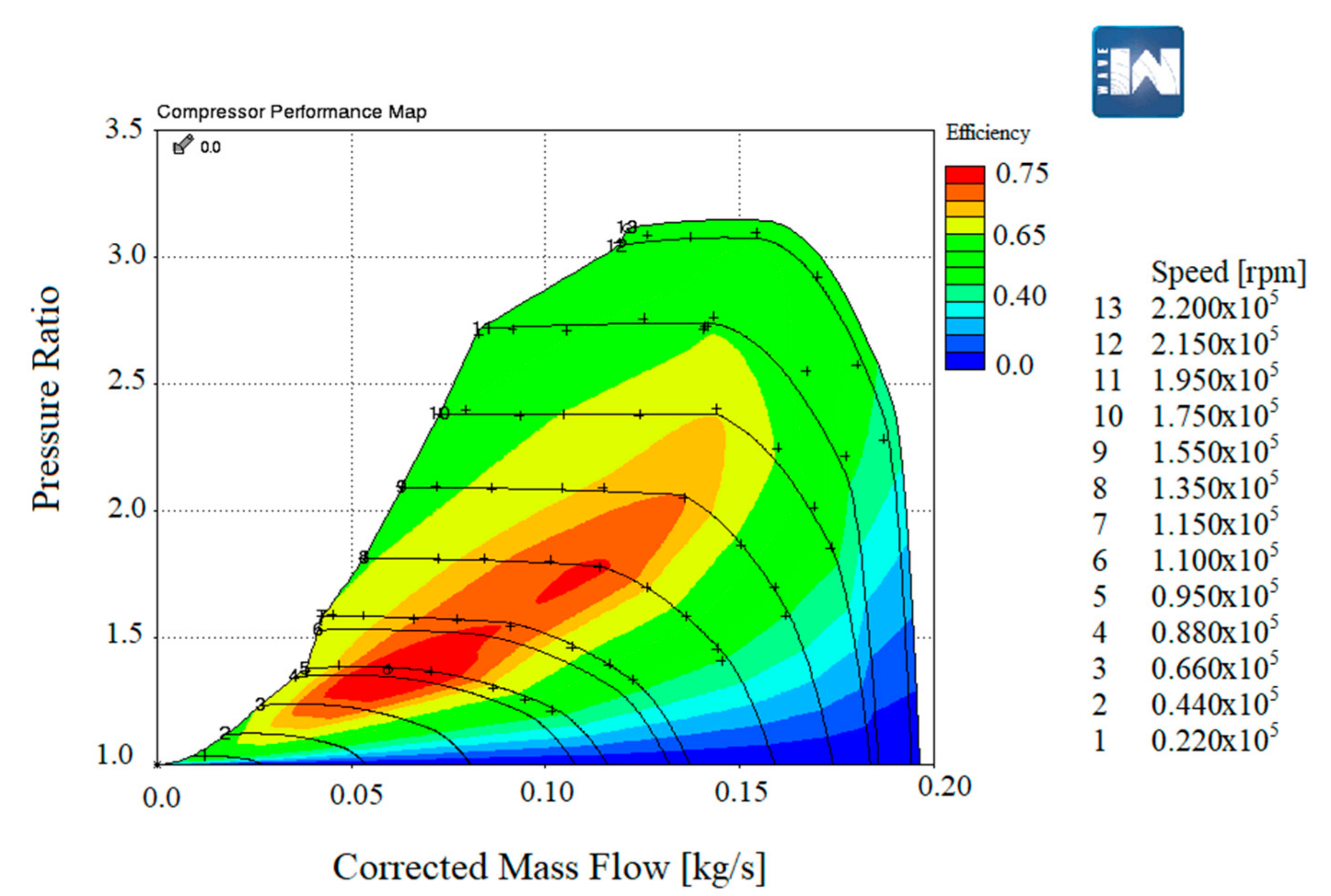
Applsci 10 07452 g001
Figure 2. Typical map of a compressor.
Applsci 10 07452 g002
Figure 3. SI Wiebe combustion model parameters.
Applsci 10 07452 g003
Figure 4. Torque and power performance of Ford Eco Boost 1.6 L petrol engine at full load.
Applsci 10 07452 g004
Figure 5. BSFC (Brake-specific fuel consumption) of Ford Eco Boost 1.6 L petrol engine at full load.
Applsci 10 07452 g005
Figure 6. Turbine Ricardo WAVE map.
Applsci 10 07452 g006
Figure 7. Compressor dimensionless map.
Applsci 10 07452 g007
Figure 8. Turbine map for different dimensionless speeds.
Applsci 10 07452 g008
Figure 9. Scaled compressor map.
Applsci 10 07452 g009
Figure 10. Scaled turbine map.
Applsci 10 07452 g010
Figure 11. Variation of engine torque during compressor speed sweep at different engine speeds.
Applsci 10 07452 g011
Figure 12. Variation of engine power during compressor speed sweep at different engine speeds.
Applsci 10 07452 g012
Figure 13. Comparison between provided engine torque and Ricardo WAVE model.
Applsci 10 07452 g013
Figure 14. Comparison between provided engine power and Ricardo WAVE model.
Applsci 10 07452 g014
Figure 15. Comparison between provided engine BSFC and Ricardo WAVE model.
Applsci 10 07452 g015
Figure 16. Variation of engine air mass flow rate during compressor speed sweep at each engine speed.
Applsci 10 07452 g016
Figure 17. Baseline engine torque at different engine speeds.
Applsci 10 07452 g017
Figure 18. Baseline engine brake power at different engine speeds.
Applsci 10 07452 g018
Figure 19. Baseline engine BSFC at different engine speeds.
Applsci 10 07452 g019
Figure 20. Baseline engine carbon monoxide emissions at different engine loads.
Applsci 10 07452 g020
Figure 21. Baseline engine NOx emissions at different engine loads.
Applsci 10 07452 g021
Figure 22. Baseline engine uHC (Unburned Hydrocarbons) emissions at different engine loads.
Applsci 10 07452 g022
Figure 23. Transient WAVE simulation component setup.
Applsci 10 07452 g023
Figure 24. Baseline time to reach maximum shaft speed at various engine speeds and loads.
Applsci 10 07452 g024
Figure 25. Mass flow rate vs. pressure ratio plots at constant shaft speeds for axial turbine.
Applsci 10 07452 g025
Figure 26. Total to static efficiency vs. pressure ratio plots at constant shaft speeds for axial turbine.
Applsci 10 07452 g026
Figure 27. Corrected mass flow rate vs. pressure ratio plots at constant shaft speeds at different rack positions for VNT (Variable Nozzle Turbine)
Applsci 10 07452 g027
Figure 28. Total to static efficiency vs. pressure ratio plots at constant shaft speeds at different rack positions for VNT.
Applsci 10 07452 g028
Figure 29. Comparison of (a) engine brake torque, (b) engine brake power, (c) engine BSFC, (d) turbine power, and (e) turbine efficiency between radial and axial turbines at different engine operating conditions.
Applsci 10 07452 g029
Figure 30. Comparison of engine cylinder emissions between radial (a,c,e) and axial turbines (b,d,f) at different engine operating conditions.
Applsci 10 07452 g030
Figure 31. Comparison between radial (left) and axial (right) turbines time to maximum shaft speed at different engine operating conditions.
Applsci 10 07452 g031
Figure 32. Transient response profiles for turbocharger shaft speed and manifold pressure at engine speeds of 5000 rpm (a,b), 4000 rpm (c,d), and 3000 rpm (e,f) at 100% (left) and 60% (right) engine loads.
Applsci 10 07452 g032
Figure 33. (a) Optimized blade design and (b) 3D model of the axial turbine.
Applsci 10 07452 g033
Table 1. Reference conditions for conducting turbocharger maps.
Reference ConditionCompressorTurbine
Pressure100101.3
Temperature298288
Table 2. Target conditions for turbocharger.
ParameterCompressor TargetTurbine Target
Ttarg411 K1170 K
Ptarg2.14 bar2.65 bar
mtarg0.118 kg/s0.127 kg/s
Table 3. Results of scaling for different engine speed performances.
Engine Speed D C   m D T   m
1000 rpm0.055710.05186
3000 rpm0.052530.05258
5000 rpm0.049850.05298
6000 rpm0.046640.05308
Table 4. Design point turbine boundary conditions generated in WAVE.
ConditionValue
Inlet total pressure (bar)2.65611
Outlet static pressure (bar)1.30352
Inlet total temperature (K)1168.55
Outlet static temperature (K)1052.44
Mass flow rate (kg/s)0.1272
Table 5. Turbocharger speed map.
NTC (rpm)Engine Speed (rpm)
Load100020003000400050006000
100%46,700106,500143,630145,210158,850141,757
80%26,97869536112,308111,906121,476111,412
60%52142475163,18264,31369,69766,690
40%n/an/a13,39521,60931,42932,202
Table 6. Air mass flow rate at each engine speed and load.
mae (kg/hr) Engine Speed (rpm)
Load100020003000400050006000
100%57.9623143.255257.264335.677427.272433.747
80%46.2953113.751207.029269.308342.331347.253
60%34.842385.4361153.386202.144256.701259.625
40%n/an/a102.079132.553167.475171.063
Table 7. Number of cycles required to complete a 3-s transient simulation for each engine speed.
Engine Speed (rpm)Number of Cycles
100025
200050
300075
4000100
5000125
6000150
Table 8. Experimentally obtained mass moment of inertia for GT1548 turbocharger.
TurbochargerTurbineCompressor
Moment of Inertia (kg/m2)Moment of Inertia (kg/m2)Moment of Inertia (kg/m2)
5.54 × 10−64.72 × 10−68.22 × 10⁻⁷
Table 9. Results of inertia testing of GT1548 turbocharger.
ParameterGT 1548 TurbochargerGT1548 Scaled TurbochargerScale Factor
Compressor diameter0.048 m0.04902 m1.02125
Turbine diameter0.0412 m0.05343 m1.29684
Compressor inertia8.22 × 10−7 kg m29.13 × 10−7 kg m2(1.02125)5
Turbine inertia4.72 × 10−6 kg m21.73 × 10−5 kg m2(1.29684)5
Turbocharger inertia5.54 × 10−6 kg m21.82 × 10−5 kg m2n/a
Table 10. Turbocharger shaft speed based on engine model operating conditions for map generation.
Engine Speed (rpm)Load (%)Turbocharger Speed (rpm)
5000100158,850
3000100143,360
500080121,476
2000100106,500
20008069,536
100010046,700
10008026,978
Table 11. Comparison of baseline radial, axial turbine, and optimised axial turbine design.
Radial TurbineAxial Turbine (Initial Design)Axial Turbine (Optimized Design)
Mass (g)226.76112.9385.41
Mass moment of inertia (kg/m2)1.82 × 10−51.59 × 10−51.16 × 10⁻⁵
Safety FactorNA2.382.16
Publisher’s Note: MDPI stays neutral with regard to jurisdictional claims in published maps and institutional affiliations.

