Design and Evaluation of a New Fuzzy Control Algorithm Applied to a Manipulator Robot

Abstract

In this article, we propose a new scheme for a fuzzy logic controller, which includes acceleration as one of its linguistic variables, as opposed to other techniques and approaches that have been developed and reported in the literature. This method is used for controlling the tracking of the trajectory followed by the joints of a 2-DoF manipulator robot. To this end, a complete simulation environment is developed through the MatLab/Simulink^® software. The dynamic model of the manipulator robot includes a vector that consists of the estimate of the friction forces present in the joints. Then, a controller based on fuzzy logic is designed and implemented for each joint. Finally, the performance of the developed system is assessed and then compared to the performance of a classic PID controller. The incorporation of the fuzzy variable acceleration significantly improved the system’s response.

1. Introduction

The performance of mechanical and routine tasks, as well as the speeding-up of processes in which precision cannot be overlooked, are just two of the most outstanding features that have made industrial robots the most preferred tool for increasing productivity and reducing operational costs.

For a robot to perform a specific movement, a control device that ensures the completion of this movement is essential. Despite the utmost importance of control in manipulator robots, control is still an issue that poses several practical and theoretical challenges to the field, due to the complex dynamic of these robots and the need to achieve highly precise trajectory-tracking in the case of high-speed movements with variable loads [1,2].

Manipulator robots are multivariable and non-linear dynamic systems. Therefore, obtaining mathematical models that both represent them and in which classic or modern control laws are satisfactorily applicable is difficult, as it is necessary to know the exact masses, inertias, and lengths of each link, as well as other characteristic parameters. Also, these robots face a series of uncertainties inherent to their practical application, such as internal friction or external disturbances. To solve such inconveniences, several control strategies have been proposed, among which the Proportional-Integral-Derivative (PID) method is widely accepted and extensively used in industrial robots. The success of this method is attributed to its simple structure and robust performance in a wide range of operating conditions. Furthermore, these controllers can minimize the steady-state error of a manipulator robot, but they are sensitive to the variation of parameters and uncertainties of the latter [3,4,5].

Conventional control techniques such as PID, adaptive control, and sliding mode control, among others, depend largely on precise mathematical modelling. These approaches may be adapted to robots operated in environments without uncertainty and with models that are exactly known; thus, the absence of an accurate analytical model makes it difficult to design an adequate controller [6,7]. Nevertheless, operations in non-structured environments, where there always will be some degree of uncertainty, require robots to carry out tasks that are more complex [8,9].

Fuzzy control is a control technique that belongs to the expert systems and that allows for controlling dynamic systems without any mathematical model. This characteristic makes fuzzy control suitable for complex processes that are difficult to model analytically, either because of the incomplete knowledge of the procedure or the unfeasibility of identifying the experimental model due to the unquantifiability of the process inputs and outputs. Thus, this technique may be understood as a mean that enables the conversion of a linguistic control strategy, which is based on the knowledge of an operator, into an automatic control strategy [10].

A controller based on fuzzy logic delivers fast and precise dynamic responses, allows for analyzing information through a true-and-false scale, and is generally robust, and tolerant to imprecisions and noise in the input data, among other characteristics. The logic programming of fuzzy controllers is governed by rules whose order is arbitrary and can be modified in number and type of membership function [11,12].

Since its creation, fuzzy logic has been widely adopted by researchers to develop controllers for a wide variety of systems in different fields. Some examples of these controllers are: the intelligent medication dispenser, which is based on the analysis of the data flow from a patient’s body temperature [13]; a robust fuzzy algorithm to analyze asthma data [14]; the use of terms and linguistic expressions to capture the human way of reasoning at different accuracy levels [15]; clustering algorithm for wireless sensor networks with five input parameters (energy, centrality, distance to base station, number of hops and node density), which is fault tolerant [16]; selection and tuning of control law parameters to pilot an Unmanned Aerial Vehicle (UAV) [17]; stabilization of an inverted pendulum on a car [18]; general scheme for controlling non-linear, uncertain and chaotic MIMO systems [19,20]; adaptation of a classic PID controller through an expert system based on fuzzy rules [21]; control of uncertain strict-feedback non-linear systems, with asymmetric output restrictions that vary over time in the presence of input saturation [22]; type-1 fuzzy logic-based controller for push recovery by humanoids [23]; Adaptive Neuro Fuzzy Inference System (ANFIS) controller for navigation of single as well as multiple mobile robots in highly cluttered environments [24], etc.

In robotics, control system algorithms based on fuzzy logic are usually calculated using information related to position and speed, which is obtained by sensors located in each of the robot joints (encoders, tachometers, etc.) [25]. The main scientific advances that employ position and speed, i.e., error and first derivative of the error with respect to time, as linguistic variables of a control system based on fuzzy logic are: (1) Hybrid control systems, comprising force/motion, force/position and fuzzy-PID; (2) Fuzzy adaptive control with obstacle avoidance and dynamic uncertainty; (3) Fuzzy adaptive control for efficient surfing of mobile robots, whose main contribution is following trajectories and avoiding obstacles; (4) Fractional order fuzzy controllers; (5) Adaptive fractional order PID controller; (6) Adaptive control methods based on PID architectures to control highly non-linear industrial processes, even under conditions of parameter variability, noise and instabilities [1,7,26,27,28,29,30,31,32,33,34,35,36].

2. Controllers

According to [37], there are several types of Fuzzy Logic Controllers (FLC) that can be built, among which the most known are FLC-PD, FLC-PI, and FLC-PID. Depending on the type of controller, the following inputs may be used: error $e$, error change $∆e$, and/or sum of errors $\sum e$.

FLC-P: The equation for a conventional proportional (P) fuzzy controller is given by:

$$u=k_p\cdot e(k)$$

(1)

where $k_p$ represents the proportional gain coefficient and $u$ the control output. The rules for a P-type FLC are built based on the following formulation: If $e$ is $A_i$ then $u$ is $B_j$, where $A_i$ and $B_j$, $i$, $j=1,2,\dots ,n.$ represent linguistic variables.

FLC-PD: A Proportional-Differential (PD) FLC can be developed by using error and error change model, as shown in the following equation:

$$u=k_p\cdot e+k_d\cdot ∆e$$

(2)

where $k_p$ and $k_d$ represent the coefficients of proportional and differential gains, and $u$ corresponds to control output. The rules for a PD-type FLC are formulated as follows: If $e$ is $A_i$ and $∆e$ is $B_j$ then $u$ is $C_k$, where $A_i$, $B_j$ and $C_k$ are linguistic variables and $i=1,2,\dots ,n_1$, $j=1,2,\dots ,n_2$ and $k=1,2,\dots ,n_3$.

FLC-PI: A conventional Proportional Integral controller is described as:

$$u=k_{p}e+k_l{\displaystyle \int edt}$$

(3)

where $k_p$ and $k_l$ are the proportional and integral gains coefficient, and $u$ is the control output. This controller is built based on the following rules: If $e$ is $A_i$ and $\sum e$ is $B_j$ then $u$ is $C_k$, where $A_i$, $B_j$ and $C_k$ are linguistic variables. This type of FLC has a good performance and reduces error in stationary state, but causes degraded rise time and settling time. These undesirable characteristics are generated by the operation of the controller’s integral, although this integrator is introduced just to overcome the issue of errors in stationary state.

FLC similar to PID: An additional option that allows for obtaining better performance in terms of rise time, settling time, overshoot and error in stationary state is to develop a PID, which is described by the following equation:

$$u_{PID}=k_p\cdot e+k_d\cdot ∆e+k_l{\displaystyle \underset{0}{\overset{t}{\int }}e\cdot dt}$$

(4)

The FLC-PID has the following rules: If $e$ is $A_i$ and $∆e$ is $B_j$ and $\sum e$ is $C_k$ then $u$ is $D_l$, where $i=1,2,\dots ,n_1$, $j=1,2,\dots ,n_2$, $k=1,2,\dots ,n_3$ and $l=1,\dots ,m.$.

In general, a two-term PD fuzzy controller is not able to eliminate error in stationary state, whereas a two-term PI-fuzzy controller is. However, the latter has a slower response due to the integral term in the control variable.

To meet the design criteria, including fast rise time, minimum overshoot, shorter settling time, and error at stationary status equal to zero, an additional option may be developed: a PID-type FLC. PID fuzzy controllers are four-dimensional (three inputs and one output) systems, whose control law is based on the error $e$, error change $∆e$, and error integral or sum $\sum e.$ Nevertheless, this FLC supports a long processing time that results in an excessively slow response, which is not suitable for applications that need a quick response, for example, the control of joint trajectory of the 2-DoF manipulator robot addressed in this study.

Several authors have proposed different approaches to overcome the problems above, such as decomposing PID FLC into a fuzzy PD connected in parallel to various types of fuzzy gains, fuzzy integrators, integral fuzzy controller, deterministic fuzzy controller; fuzzy PD with gain control in stationary state; fuzzy PD with integral action control; fuzzy PD with fuzzy integral gain controller; fuzzy PD and PI combined, and fuzzy PD and I combined. All these configurations and their corresponding schemes are shown in [37].

None of these approaches include the error second derivative $\ddot{e}$, nor are other applications with these characteristics found in the literature. This characteristic allows for obtaining representative improvements when assessing the results from joint trajectory tracking in manipulator robots (results were validated based on the calculation of performance indexes), and comparing them with results from conventional fuzzy and PID controllers. It must be noted that adding the error second derivative to the proposed fuzzy controller makes this study original and therefore a contribution to the manipulator robot’s control.

The new scheme we propose is applied to the control of the joint trajectory tracking of a 2-DoF planar robot, for which a complete simulation environment is developed using the software MatLab/Simulink^®. Finally, a performance assessment is presented, which consists of a comparison between the fuzzy controller and a classic PID controller (the classic PID controller is only used for comparison).

3. Manipulator Robot Model

The following general notation is considered to obtain the dynamic model of a 2-DoF planar manipulator robot with $i=1,2,\dots ,n.$ joints and q generalized coordinates [3,38]:

$$\tau \hspace{0.17em}\hspace{0.17em}\hspace{0.17em}\hspace{0.17em}=\hspace{0.17em}\hspace{0.17em}\hspace{0.17em}\hspace{0.17em}M\left(q\right)\ddot{q}\hspace{0.17em}\hspace{0.17em}+\hspace{0.17em}\hspace{0.17em}C\left(q,\dot{q}\right)\hspace{0.17em}\hspace{0.17em}+\hspace{0.17em}\hspace{0.17em}G\left(q\right)+F\left(\dot{q}\right)$$

(5)

where:

τ:	Generalized forces vector (n×1 dimension).
M:	Inertia matrix (n×n dimension).
C:	Centrifuge and Coriolis force vectors (n×1 dimension).
G:	Gravitational force vector (n×1 dimension).
F:	Friction force vector (n×1 dimension).
$\ddot{q}$:	Joint acceleration vector (n×1 dimension).
$q$:	Components of the joint position vector.
$\dot{q}$:	Components of the joint speed vector.

Figure 1 shows the scheme of the 2-DoF planar manipulator robot used, which includes the location of the centroids (mass centers) of each link. According to Equation (1), which is based on the Lagrange-Euler formulation, the dynamic model of the manipulator may be expressed through Equations (6) to (17) [3,38]:

$$M=\left[\begin{array}{cc}{M}_{11}& M_{12}\\ M_{21}& M_{22}\end{array}\right]$$

(6)

$$M_{11}=m_1\cdot l_{c1}^2+m_2\cdot \left[l_1^2+l_{c2}^2+2\cdot l_1\cdot l_{c2}\cdot \cos \left({\theta }_2\right)\right]+I_1+I_2$$

(7)

$$M_{12}=m_2\cdot l_1\cdot l_{c2}\cdot \cos \left({\theta }_2\right)+m_2\cdot l_{c2}^2+I_2$$

(8)

$$M_{21}=m_2\cdot l_1\cdot l_{c2}\cdot \cos \left({\theta }_2\right)+m_2\cdot l_{c2}^2+I_2$$

(9)

$$M_{22}=m_2\cdot l_{c2}^2+I_2$$

(10)

$$C=\left[\begin{array}{c}{C}_{11}\\ C_{21}\end{array}\right]$$

(11)

$$C_{11}=-m_2\cdot l_1\cdot l_{c2}\cdot \sin \left({\theta }_2\right)\cdot {\dot{\theta }}_2^2-2\cdot m_2\cdot l_1\cdot l_{c2}\cdot \sin \left({\theta }_2\right)\cdot {\dot{\theta }}_1\cdot {\dot{\theta }}_2$$

(12)

$$C_{21}=m_2\cdot l_1\cdot l_{c2}\cdot \sin \left({\theta }_2\right)\cdot {\dot{\theta }}_1^2$$

(13)

$$G=\left[\begin{array}{c}{G}_{11}\\ G_{21}\end{array}\right]$$

(14)

$$G_{11}=\left\{m_1\cdot l_{c1}\cdot \cos \left({\theta }_1\right)+m_2\cdot \left[l_1\cdot \cos \left({\theta }_1\right)+l_{c2}\cdot \cos \left({\theta }_1+{\theta }_2\right)\right]\right\}\cdot g$$

(15)

$$G_{21}=\left[m_2\cdot l_{c2}\cdot \cos \left({\theta }_1+{\theta }_2\right)\right]\cdot g$$

(16)

$$F=\left[\begin{array}{c}{F}_{11}\\ F_{21}\end{array}\right]$$

(17)

where:

m1:	Mass of the first link.	[kg]
m2:	Mass of the second link.	[kg]
l1:	Length of the first link.	[m]
l2:	Length of the second link.	[m]
lc1:	Length from the origin of the first link to its centroid.	[m]
lc2:	Length from the origin of the second link to its centroid.	[m]
I1:	Moment of inertia of the first link with respect to the first z axis of its joint.	[kg·m2]
I2:	Moment of inertia of the second link with respect to the first z axis of its joint.	[kg·m2]

Table 1. Manipulator robot parameters.

Link 1	Link 2	Units
m1 = 0.392924	m2 = 0.094403	$\left[\mathrm{kg}\right]$
l1 = 0.2032	l2 = 0.1524	$\left[\mathrm{m}\right]$
lc1 = 0.104648	lc2 = 0.081788	$\left[\mathrm{m}\right]$
I1 = 0.0011411	I2 = 0.0020247	$\left[\mathrm{kg}\cdot {\mathrm{m}}^2\right]$
Fv1 = 0.141231	Fv2 = 0.3530776	$\left[\frac{\mathrm{N}\cdot \mathrm{m}\cdot \mathrm{s}}{\mathrm{rad}}\right]$
Feca1 = 0.05	Feca2 = 0.05	$\left[\mathrm{N}\cdot \mathrm{m}\right]$
Fecb1 = 0.05	Fecb2 = 0.05	$\left[\mathrm{N}\cdot \mathrm{m}\right]$

shows the parameter values considered for each link of the manipulator robot [1,38].

4. Manipulator Robot Simulation

An adequate simulation that shows the capacity of a controller to follow the joint trajectory of a robot requires a precise design of the manipulator robot’s mathematical model, as this model provides its kinematic and dynamic characteristics. These characteristics are represented by equations shown in Section 2.

From Equation (5), obtained through the Lagrange-Euler formulation, it may be deduced that:

$$\ddot{q}\hspace{0.17em}\hspace{0.17em}\hspace{0.17em}\hspace{0.17em}=\hspace{0.17em}\hspace{0.17em}\hspace{0.17em}\hspace{0.17em}{M}^{-1}\left(q\right)\hspace{0.17em}\left[\tau \hspace{0.17em}-C\left(q,\dot{q}\right)\hspace{0.17em}\hspace{0.17em}-\hspace{0.17em}\hspace{0.17em}G\left(q\right)-F\left(\dot{q}\right)\right]\hspace{0.17em}$$

(18)

Equation (18) is applied in the MatLab/Simulink software to simulate the dynamics of the 2-DoF manipulator robot, whose block diagram is shown in Figure 2. The internal structure of each module is as follows: inertia matrix (inverse, i.e., M ^ − 1); robot’s friction force estimation vector (F(q’)); Centrifugal and Coriolis force vectors (C(q,q’)); and gravitational force vector (G(q)). This structure is based on an Embedded MATLAB Function, in which are introduced the corresponding equation with the parameter values shown in Table (matrix or vector equations are shown in Section 2).

As observed in Figure 2, the block diagram delivers the following variables: position q, speed q’, and acceleration q’’. In addition, it needs the variable “tau” as an input, which comes from the actuators block. In this work, the actuators used are direct current servomotors whose dynamic model is developed in [39].

Finally, the complete structure of the 2-DoF manipulator robot is displayed in Figure 3.

5. Fuzzy Logic Controller Design

The block diagram shown in Figure 4 represents the general structure of a fuzzy logic controller. This controller has three main components: 1. Fuzzification block, in charge of the transformation of each input element into membership degrees for the linguistic terms of the fuzzy sets, each of which has a membership function associated with its elements, indicating to what extent the element is part of the set; 2. Inference engine, which along with the knowledge base makes decisions −based on the membership degree of the input data from the fuzzy sets− and delivers output fuzzy sets that are calculated using the rules of the controller; 3. Defuzzification block that transforms fuzzy values −obtained from the inference− into values that are useful for the process to be controlled.

The output for each fuzzy controller is governed by the defuzzification process and its rule base. The defuzzification process transforms the fuzzy sets into exact values that feed the plant and depend on two Fuzzy Inference Systems (FIS). These systems are applied to achieve appropriate control actions based on assigning two rules: Mamdani and Takagi-Sugeno (TS) [18]. The main difference between the two methods lies in the consequence of fuzzy rules. Mamdani inference systems use fuzzy sets, while TS systems employ linear functions of input variables as a consequence of the rule [40,41]. The rule structure of the Mamdani-type FIS is expressed as follows: IF x₁ is A₁ and x₂ is A₂ and ... and x_n is A_n THEN y is B, where x_i (i = 1, 2 ... n) are input variables and y is the output variable; A₁ ... A_n and B (linguistic terms) are used to define the distribution of the membership function of fuzzy subsets corresponding to the input and output variables [41]. The crisp output of a Mamdani FIS is obtained when applying one of the following defuzzification methods [40,42].

Mass center, area or centroid: This technique takes the output distribution and finds its mass center to obtain a crisp number through the following equation:

$$z=\frac{{\displaystyle {\sum }_{j=1}^q{Z}_j{\mu }_c(Z_j)}}{{\displaystyle {\sum }_{j=1}^q{\mu }_c(Z_j)}}$$

(19)

where $z$ is the center of mass and ${\mu }_c$ is the membership in class c at value $z_j.$.

Maximum value mean: This technique takes the output distribution and finds the mean of its maximum values to obtain a crisp number through the following equation:

$$z={\displaystyle \sum _{j=1}^l\frac{z_j}{l}}$$

(20)

where $z$ is the mean of maximum values, $z_j$ is the point at which the membership function reaches its maximum, and $l$ is the number of times the output distribution reaches the maximum level. This work uses a Mamdani FIS with the max-min composition rule and the centroid method.

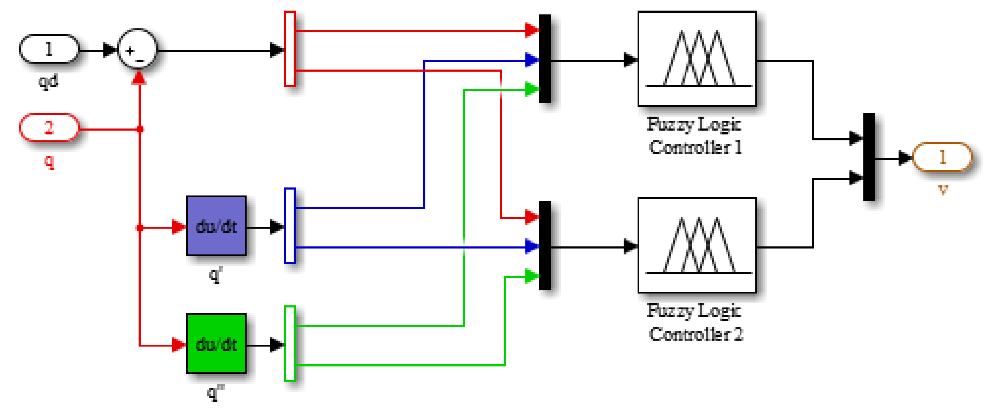
The control scheme designed for this scenario and simulated in Simulink^® is shown in Figure 5. It includes two fuzzy logic controllers, one for each joint of the manipulator robot. In addition, each fuzzy block receives three fuzzy inputs. The first input corresponds to position and represents the difference between the desired position qd and the real position q. The following input corresponds to speed q’ (first derivative of position with respect to time) and the last one represents q’’ acceleration (second derivative of position with respect to time). Additionally, each block has only one fuzzy output that represents the voltage received by the actuator. The magnitude of this voltage generates the torque force necessary for moving the respective joint.

The universes of each fuzzy variable are determined through the analysis of the simulations conducted with a test trajectory. However, the universe of the variable “position” (expressed in radians) is the maximum joint movement of each joint, while the universes of the variables speed, acceleration and voltage are defined based on the technical specifications of the actuators used.

Table 2. Characteristics of the fuzzy variables of the Fuzzy Logic Controller 1.

Fuzzy Logic Controller 1 Characteristics
Name	Position	Speed	Acceleration	Voltage
Universe	[−2 2]	[−5 5]	[−2 2]	[−19 19]
Terms	NB, NS, Z, PS, PB	LVF, LF, S, RF, RVF	N, Z, P	LB, LS, Z, RS, RB
Significators	Several	Several	Several	Several

and

Table 3. Characteristics of the fuzzy variables of the Fuzzy Logic Controller 2.

Fuzzy Logic Controller 2 Characteristics
Name	Position	Speed	Acceleration	Voltage
Universe	[−2 2]	[−5 5]	[−1 1]	[−19 19]
Terms	NB, NS, Z, PS, PB	LVF, LF, S, RF, RVF	N, Z, P	LB, LS, Z, RS, RB
Significators	Several	Several	Several	Several

show the characteristics of the variables of each controller. In these tables the terms NB, NS, Z, PS and PB correspond to Negative Big, Negative Small, Zero, Positive Small and Positive Big, respectively. On the other hand, LVF, LF, S, RF and RVF represent Left Very Fast, Left Fast, Slow, Right Fast, Right Very Fast, accordingly; N, Z and P correspond to Negative, Zero and Positive, and LB, LS, Z, RS and RB to Left Big, Left Small, Zero, Right Small and Right Big.

Fuzzy rules express the previous knowledge on the relation between antecedents and consequents (input and output fuzzy sets). The rule base can be stored as a Fuzzy Associative Memory (FAM). FAMs are matrices that represent the consequence of each rule defined for each two-input combination [37,40].

Theoretically, the number of rules necessary for gathering all the possible input combinations for a three-term fuzzy controller is obtained by: $n_1\times n_2\times n_3$, where $n_1$, $n_2$ and $n_3$ are the number of linguistic terms of the three input variables. Specifically, if $n_1=n_2=n_3=5$, then the number of rules would be: R = 5 × 5 × 5 = 125. In practical applications, the design and implementation of a fuzzy controller with such a big number of rules is a tedious task that also requires substantial space in memory and long processing time [37].

Therefore, we propose two FAMs for this controller, each with two different inputs, but with the same output (the voltage that enters the actuators). FAM 1 and FAM 2 combine speed and position inputs, while FAM 3 combines position and acceleration inputs. Both FAMs are shown in

Table 4. FAM 1 (join 1).

	Speed
Position	LVF	LF	S	RF	RVF
NB	LS	Z	LB	LB	LB
NS	RB	LS	LB	LB	LB
Z	RB	RS	Z	LS	LB
PS	RB	RB	RB	RS	LB
PB	RB	RB	RB	RS	Z

and

Table 5. FAM 2 (join 2).

	Speed
Position	LVF	LF	S	RF	RVF
NB	LB	LB	LB	LB	LB
NS	RB	LS	LB	LB	LB
Z	RB	RS	Z	LS	LB
PS	RB	RB	RB	RS	LB
PB	RB	RB	RB	RS	Z

, respectively.

After different tests and result analysis, 12 out of the 15 possible combinations for FAM 3 were suppressed because they did not improve trajectory tracking under any conditions. For this reason, in

Table 6. FAM 3 (join 1 and join 2).

	Acceleration
Position	N	Z	P
NB	x	x	x
NS	x	x	LS
Z	x	Z	x
PS	RS	x	x
PB	x	x	x

most of the elements present in FAM 3 are represented by the letter x, which corresponds to the value of excluded consequents.

The rule base shown in

Table 7. Fuzzy Logic Controller 1 rule base.

IF (Position is NB) and (Velocity is LVF)	Then (Voltage is LS)
IF (Position is NB) and (Velocity is LF)	Then (Voltage is Z)
IF (Position is NB) and (Velocity is S)	Then (Voltage is LB)
IF (Position is NB) and (Velocity is RF)	Then (Voltage is LB)
IF (Position is NB) and (Velocity is RVF)	Then (Voltage is LB)
IF (Position is NS) and (Velocity is LVF)	Then (Voltage is RB)
IF (Position is NS) and (Velocity is LF)	Then (Voltage is LS)
IF (Position is NS) and (Velocity is S)	Then (Voltage is LB)
IF (Position is NS) and (Velocity is RF)	Then (Voltage is LB)
IF (Position is NS) and (Velocity is RVF)	Then (Voltage is LB)
IF (Position is Z) and (Velocity is LVF)	Then (Voltage is RB)
IF (Position is Z) and (Velocity is LF)	Then (Voltage is RS)
IF (Position is Z) and (Velocity is S)	Then (Voltage is Z)
IF (Position is Z) and (Velocity is RF)	Then (Voltage is LS)
IF (Position is Z) and (Velocity is RVF)	Then (Voltage is LB)
IF (Position is PS) and (Velocity is LVF)	Then (Voltage is RB)
IF (Position is PS) and (Velocity is LF)	Then (Voltage is RB)
IF (Position is PS) and (Velocity is S)	Then (Voltage is RB)
IF (Position is PS) and (Velocity is RF)	Then (Voltage is RS)
IF (Position is PS) and (Velocity is RVF)	Then (Voltage is LB)
IF (Position is PB) and (Velocity is LVF)	Then (Voltage is RB)
IF (Position is PB) and (Velocity is LF)	Then (Voltage is RB)
IF (Position is PB) and (Velocity is S)	Then (Voltage is RB)
IF (Position is PB) and (Velocity is RF)	Then (Voltage is RS)
IF (Position is PB) and (Velocity is RVF)	Then (Voltage is Z)
IF (Position is Z) and (Acceleration is Z)	Then (Voltage is Z)
IF (Position is NS) and (Acceleration is P)	Then (Voltage is LS)
IF (Position is PS) and (Acceleration is N)	Then (Voltage is RS)

is built based on the combination of the results yielded by FAM 1 and FAM 3, and this procedure is also applied to obtain the rule base presented in

Table 8. Fuzzy Logic Controller 2 rule base.

IF (Position is NB) and (Velocity is LVF)	Then (Voltage is LB)
IF (Position is NB) and (Velocity is LF)	Then (Voltage is LB)
IF (Position is NB) and (Velocity is S)	Then (Voltage is LB)
IF (Position is NB) and (Velocity is RF)	Then (Voltage is LB)
IF (Position is NB) and (Velocity is RVF)	Then (Voltage is LB)
IF (Position is NS) and (Velocity is LVF)	Then (Voltage is RB)
IF (Position is NS) and (Velocity is LF)	Then (Voltage is LS)
IF (Position is NS) and (Velocity is S)	Then (Voltage is LB)
IF (Position is NS) and (Velocity is RF)	Then (Voltage is LB)
IF (Position is NS) and (Velocity is RVF)	Then (Voltage is LB)
IF (Position is Z) and (Velocity is LVF)	Then (Voltage is RB)
IF (Position is Z) and (Velocity is LF)	Then (Voltage is RS)
IF (Position is Z) and (Velocity is S)	Then (Voltage is Z)
IF (Position is Z) and (Velocity is RF)	Then (Voltage is LS)
IF (Position is Z) and (Velocity is RVF)	Then (Voltage is LB)
IF (Position is PS) and (Velocity is LVF)	Then (Voltage is RB)
IF (Position is PS) and (Velocity is LF)	Then (Voltage is RB)
IF (Position is PS) and (Velocity is S)	Then (Voltage is RB)
IF (Position is PS) and (Velocity is RF)	Then (Voltage is RS)
IF (Position is PS) and (Velocity is RVF)	Then (Voltage is LB)
IF (Position is PB) and (Velocity is LVF)	Then (Voltage is RB)
IF (Position is PB) and (Velocity is LF)	Then (Voltage is RB)
IF (Position is PB) and (Velocity is S)	Then (Voltage is RB)
IF (Position is PB) and (Velocity is RF)	Then (Voltage is RS)
IF (Position is PB) and (Velocity is RVF)	Then (Voltage is Z)
IF (Position is Z) and (Acceleration is Z)	Then (Voltage is Z)
IF (Position is NS) and (Acceleration is P)	Then (Voltage is LS)
IF (Position is PS) and (Acceleration is N)	Then (Voltage is RS)

yielded by FAM 2 and FAM 3.

The membership functions selected for the position, speed, acceleration and voltage of the Fuzzy Logic Controller 1 are shown in Figure 6. Additionally, the 28 resulting rules entered in the rule editor of the fuzzy logic toolbox are presented in Table 7. Likewise, the membership functions chosen for the Fuzzy Logic Controller 2 are exposed in Figure 7. In this case, there are also 28 rules depicted in Table 8. Both membership functions and the rule base for each controller were built after several test simulations. These tests were carried out considering the slope changes in the position curves a priority. In this way, it was determined that by making the position and voltage sets more selective around zero, test trajectory tracking presented a performance with less tracking error for both joints.

Initially, the membership functions designed were the same for both joints. However, after the selectivity adjustments for the position and voltage sets around zero, the second joint deviated a bit more from the trajectory of the first one. This was solved by modifying the LS and RS voltage sets of the second joint, changing the soft shapes of those sets into triangular ones.

Finally, a flowchart representing the computing process for fuzzy control is shown in Figure 8.

6. Classic PID Controller

In this section, the outcomes of a PID controller simulation are presented in order to compare them to the performance of the fuzzy control scheme designed in this work. The PID control law may be expressed as:

$$\tau =K_{p}e+K_v\dot{e}+K_i{\displaystyle {\int }_0^{t}e(\sigma )d\sigma }$$

(21)

where $K_p$ represents the proportional gain, $K_v$ the derivative gain, and $K_i$ the integral gain. Using this control law, the scheme shown in Figure 9 is designed and simulated. As in the fuzzy system, two PIDs controllers (PID1 and PID2) are required, because each robot joint is controlled separately. The parameter values of this controller are K_p = 10, K_v = 0.5, K_i = 0.2. These values were obtained using the software tool PID Autotuning Toolbox from MatLab-Simulink. Different auto-tuning trials were conducted, and the values of the parameters associated with the best performance result from the PID controller were selected.

7. Simulation Results

This section presents the simulation results of the fuzzy and PID control strategies. Furthermore, the test trajectories used are shared, and then the performance of the designed controllers is assessed through three performance indicators, namely Residual Mean Square (RMS), Residual Standard Deviation (RSD), and Index of Agreement (IA).

7.1. Test Trajectories

The three qd joint trajectories considered are shown in Figure 10. Each of them lasts 8 s.

7.2. Results: Fuzzy Logic Controller with Acceleration vs. PID Controller

The control results of the desired joint trajectory-tracking achieved by the controllers (fuzzy logic vs. PID) are presented simultaneously in Figure 11—trajectory 1, Figure 12—trajectory 2, and Figure 13—trajectory 3. Each figure has a legend that indicates the desired qd and real q trajectories for the two joints of a 2-DoF planar robot.

7.3. Results: Fuzzy Controller with and without Acceleration

To elucidate how the acceleration variable affects the quality of the proposed controller, a first fuzzy controller is presented based only on the variables position and speed. Then, a second controller is presented based on position, speed and acceleration. Below are shown the error results for the trajectory-tracking of the robot’s joints, which were obtained from the controllers designed. Each figure includes a caption indicating the controller used and the number of the trajectory: Figure 14—trajectory 1, Figure 15—trajectory 2, and Figure 16—trajectory 3.

7.4. Performance Indicators

The indicators used for assessing the performance of the controllers designed in this work are shown in Equations (22)–(24), which correspond to the RMS, RSD and IA, accordingly.

$$\mathrm{RMS}=\sqrt{\frac{{\displaystyle \sum _{i=1}^n{(o_i-p_i)}^2}}{n}}$$

(22)

$$\mathrm{RSD}=\sqrt{\frac{{\displaystyle \sum _{i=1}^n{(o_i-p_i)}^2}}{{\displaystyle \sum _{i=1}^n{o}_i^2}}}$$

(23)

$$\mathrm{IA}=1-\frac{{\displaystyle \sum _{i=1}^n{(o_i-p_i)}^2}}{{\displaystyle \sum _{i=1}^n{(\left|o_i{}^{’}\right|-\left|p_i{}^{’}\right|)}^2}}$$

(24)

$$\begin{array}{l}{p}_i{}^{’}=p_i-o_m\\ o_i{}^{’}=o_i-o_m\end{array}$$

where $o_i$ represents the observed values; $p_i$ the predicted values; $o_m$ the mean value of the observations and n the total number of observations.

The values of RMS, RSD and IA calculated for joints 1 and 2 with each controller are shown in

Table 9. Calculated performance indicators: fuzzy with acceleration vs. PID.

Controller	Indicator	Trajectory 1		Trajectory 2		Trajectory 3
		Joint 1	Joint 2	Joint 1	Joint 2	Joint 1	Joint 2
Fuzzy with acceleration	RMS	0.0120	0.0156	0.0430	0.2397	0.3044	0.2478
	RSD	0.0130	0.0167	0.0390	0.2288	0.4515	0.4498
	IA	0.9997	0.9995	0.9996	0.9871	0.8977	0.9246
PID	RMS	0.0523	0.0528	0.0931	0.3069	0.3375	0.2893
	RSD	0.0588	0.0587	0.0905	0.3304	0.5949	0.6161
	IA	0.9937	0.9946	0.9980	0.9761	0.8246	0.8645

and

Table 10. Calculated performance indicators: fuzzy with acceleration vs. fuzzy without acceleration.

Controller	Indicator	Trajectory 1		Trajectory 2		Trajectory 3
		Joint 1	Joint 2	Joint 1	Joint 2	Joint 1	Joint 2
Fuzzy with acceleration	RMS	0.0120	0.0156	0.0430	0.2397	0.3044	0.2478
	RSD	0.0130	0.0167	0.0390	0.2288	0.4515	0.4498
	IA	0.9997	0.9995	0.9996	0.9871	0.8977	0.9246
Fuzzy without acceleration	RMS	0.0118	0.015	0.1757	0.301	0.3895	0.3292
	RSD	0.0127	0.016	0.1663	0.3014	0.5439	0.5564
	IA	0.9997	0.9996	0.9931	0.9782	0.8175	0.8659

.

Ideally, the RMS and RSD values should be close to 0, while IA values should be very close to 1. These results are illustrated in Figure 17 and Figure 18.

8. Conclusions

Several authors agree that the use of a controller based on fuzzy logic is a very good choice for controlling non-linear systems with mathematical models difficult to represent. This factor, along with the structure of these controllers and the possibility of selecting the membership functions as well as the ranges of the fuzzy sets to be used, yields a wide variety of results that allows for improving the performance of the system to be controlled.

In this work, we developed a fuzzy logic application for controlling the trajectory-tracking of the joints of a 2-DoF planar manipulator robot. The results of the three test trajectories have evidenced that the controllers developed satisfactorily meet the tracking control requirements. Nevertheless, the performance of the fuzzy logic controllers is visibly superior to the performance of the classic PID controller. The values of these indicators reveal that the three tested trajectories are less accurate with the PID controller. However, trajectory number three is much harder to follow, since the joints of the manipulator robot are forced to change the direction of their motion to 90° angles in very short time lapses.

The main contribution of this study was the incorporation of the acceleration fuzzy variable, which allowed for noticeably improving system response. In total, we worked with three variables: position, speed and acceleration, each of them with its respective membership functions and fuzzy sets.

The design and analyses of fuzzy controllers for manipulator robots are envisaged as future works. This should incorporate, in addition to the joint acceleration variable, the error integral variable with adaptive reset in order to improve the transient and stationary behavior in the presence of load disturbances in the second joint. Furthermore, the dynamic model of the manipulator robot could be improved by adding the Stribeck effect through modeling with a first-order non-linear differential equation.

References

1. Sharma, R.; Gaur, P.; Mittal, A.P. Design of two-layered fractional order fuzzy logic controllers applied to robotic manipulator with variable payload. Appl. Soft Comput. J. 2016, 47, 565–576. [Google Scholar] [CrossRef]
2. Hu, H.; Wang, X.; Chen, L. Impedance with Finite-Time Control Scheme for Robot-Environment Interaction. Math. Probl. Eng. 2020, 2020, 2796590. [Google Scholar] [CrossRef]
3. Urrea, C.; Saa, D. Design and Implementation of a Graphic Simulator for Calculating the Inverse Kinematics of a Redundant Planar Manipulator Robot. Appl. Sci. Basel 2020, 10, 1–18. [Google Scholar]
4. Saleki, A.; Mehdi, M. Model-free control of electrically driven robot manipulators using an extended state observer. Comput. Electr. Eng. 2020, 87, 106768. [Google Scholar] [CrossRef]
5. Rossomando, F.; Serrano, E.; Soria, C.; Scaglia, G. Neural Dynamics Variations Observer Designed for Robot Manipulator Control Using a Novel Saturated Control Technique. Math. Probl. Eng. 2020, 2020, 3240210. [Google Scholar] [CrossRef]
6. Urrea, C.; Pascal, J. Design, Simulation, Comparison and Evaluation of Parameter Identification Methods for an Industrial Robot. Comput. Electr. Eng. 2018, 67, 791–806. [Google Scholar] [CrossRef]
7. Chatterjee, A.; Watanabe, K. An adaptive fuzzy strategy for motion control of robot manipulators. Soft Comput. 2005, 9, 185–193. [Google Scholar] [CrossRef]
8. Si, G.; Chu, M.; Zhang, Z.; Li, H.; Zhang, X. Integrating Dynamics into Design and Motion Optimization of a 3-PRR Planar Parallel Manipulator with Discrete Time Transfer Matrix Method. Math. Probl. Eng. 2020, 2020, 2761508. [Google Scholar] [CrossRef]
9. Peng, J.; Yang, Z.; Ma, T. Position/Force Tracking Impedance Control for Robotic Systems with Uncertainties Based on Adaptive Jacobian and Neural Network. Complexity 2019, 2019, 1406534. [Google Scholar] [CrossRef]
10. Baghli, F.Z.; Bakkali, E.L.; Lakhal, Y. Multi-input multi-output fuzzy logic controller for complex system: Application on two-links manipulator. Procedia Technol. 2015, 19, 607–614. [Google Scholar] [CrossRef] [Green Version]
11. Bhatia, V.; Kalaichelvi, V.; Karthikeyan, R. Application of a Novel Fuzzy Logic Controller for a 5-DOF Articulated Anthropomorphic Robot. In Proceedings of the 2015 IEEE International Conference on Research in Computational Intelligence and Communication Networks (ICRCICN), Kolkata, India, 20–22 November 2015; pp. 208–213. [Google Scholar]
12. Ghanooni, P.; Yazdanib, A.M.; Mahmoudi, A.; MahmoudZadeh, S.; Ahmadi Movaheded, M.; Fathi, M. Robust precise trajectory tracking of hybrid stepper motor using adaptive critic-based neuro-fuzzy controller. Comput. Electr. Eng. 2020, 81, 106535. [Google Scholar] [CrossRef]
13. Medina, J.; Espinilla, M.; García-Fernández, A.L.; Martínez, L. Intelligent multi-dose medication controller for fever: From wearable devices to remote dispensers. Comput. Electr. Eng. 2018, 65, 400–412. [Google Scholar] [CrossRef] [Green Version]
14. Yang, M.-R.; Lee, Z.-J.; Lee, C.-Y.; Peng, B.-Y.; Huang, H. An Intelligent Algorithm Based on Bacteria Foraging Optimization and Robust Fuzzy Algorithm to Analyze Asthma Data. Int. J. Fuzzy Syst. 2017, 19, 1181–1189. [Google Scholar] [CrossRef]
15. Montserrat-Adell, J.; Agell, N.; Sánchez, M.; Prats, F.; Ruiz, F.J. Modeling group assessments by means of hesitant fuzzy linguistic term sets. J. Appl. Log. 2017, 23, 40–50. [Google Scholar] [CrossRef] [Green Version]
16. Alaybeyoglu, A. A distributed fuzzy logic-based root selection algorithm for wireless sensor networks. Comput. Electr. Eng. 2017, 41, 216–225. [Google Scholar] [CrossRef]
17. Garcia-Aunon, P.; Peñas, M.S.; de la Cruz García, J.M. Parameter selection based on fuzzy logic to improve UAV path-following algorithms. J. Appl. Log. 2017, 24, 62–75. [Google Scholar] [CrossRef]
18. Roose, A.I.; Yahya, S.; Al-Rizzo, H. Fuzzy-logic control of an inverted pendulum on a cart. Comput. Electr. Eng. 2017, 61, 31–47. [Google Scholar] [CrossRef]
19. Mahmoodabadi, M.J.; Abedzadeh Maafi, R.; Taherkhorsandi, M. An optimal adaptive robust PID controller subject to fuzzy rules and sliding modes for MIMO uncertain chaotic systems. Appl. Soft Comput. 2017, 52, 1191–1199. [Google Scholar] [CrossRef]
20. Iqbal Ahammed, A.K. Profoundly Robust Controlling Strategy for Uncertain Nonlinear Mimo System Using T--S Fuzzy System. Int. J. Fuzzy Syst. 2017, 19, 1104–1117. [Google Scholar] [CrossRef]
21. Nowaková, J.; Pokorný, M.; Pieš, M. Conventional controller design based on Takagi–Sugeno fuzzy models. J. Appl. Log. 2015, 13, 148–155. [Google Scholar] [CrossRef]
22. Edalati, L.; Khaki Sedigh, A.; Aliyari Shooredeli, M.; Moarefianpour, A. Adaptive fuzzy dynamic surface control of nonlinear systems with input saturation and time-varying output constraints. Mech. Syst. Signal Process. 2018, 100, 311–329. [Google Scholar] [CrossRef]
23. Semwal, V.B.; Chakraborty, P.; Nandi, G.C. Less computationally intensive fuzzy logic (type-1)-based controller for humanoid push recovery. Rob. Auton. Syst. 2015, 63, 122–135. [Google Scholar] [CrossRef]
24. Pothal, J.K.; Parhi, D.R. Navigation of multiple mobile robots in a highly clutter terrains using adaptive neuro-fuzzy inference system. Rob. Auton. Syst. 2015, 72, 48–58. [Google Scholar] [CrossRef]
25. Bueno López, M.; Arteaga Pérez, M. Fuzzy logic control of a robot manipulator in 3D based on visual servoing. IFAC Proc. 2011, 44, 14578–14583. [Google Scholar] [CrossRef]
26. Bakdi, A.; Hentout, A.; Boutami, H.; Maoudj, A.; Hachour, O.; Bouzouia, B. Optimal path planning and execution for mobile robots using genetic algorithm and adaptive fuzzy-logic control. Rob. Auton. Syst. 2017, 89, 95–109. [Google Scholar] [CrossRef]
27. Karray, A.; Njah, M.; Feki, M.; Jallouli, M. Intelligent mobile manipulator navigation using hybrid adaptive-fuzzy controller. Comput. Electr. Eng. 2016, 56, 773–783. [Google Scholar] [CrossRef]
28. Kumar, A.; Kumar, V. Hybridized ABC-GA optimized fractional order fuzzy pre-compensated FOPID control design for 2-DOF robot manipulator. AEU Int. J. Electron. Commun. 2017, 79, 219–233. [Google Scholar] [CrossRef]
29. Jesus, I.S.; Barbosa, R.S. Smith-fuzzy fractional control of systems with time delay. AEU Int. J. Electron. Commun. 2017, 78, 54–63. [Google Scholar] [CrossRef]
30. Sharma, R.; Rana, K.P.; Kumar, V. Performance analysis of fractional order fuzzy PID controllers applied to a robotic manipulator. Expert Syst. Appl. 2014, 41, 4274–4289. [Google Scholar] [CrossRef]
31. Arpaci, H.; Ozguven, O.F. Design of Adaptive Fractional-Order PID Controller to Enhance Robustness by Means of Adaptive Network Fuzzy Inference System. Int. J. Fuzzy Syst. 2017, 19, 1118–1131. [Google Scholar] [CrossRef]
32. Seyedtabaii, S. Modified adaptive second order sliding mode control: Perturbed system response robustness. Comput. Electr. Eng. 2020, 81, 106536. [Google Scholar] [CrossRef]
33. Mendes, N.; Neto, P. Indirect adaptive fuzzy control for industrial robots: A solution for contact applications. Expert Syst. Appl. 2015, 42, 8929–8935. [Google Scholar] [CrossRef]
34. Benzaoui, M.; Chekireb, H.; Tadjine, M.; Boulkroune, A. Trajectory tracking with obstacle avoidance of redundant manipulator based on fuzzy inference systems. Neurocomputing 2016, 196, 23–30. [Google Scholar] [CrossRef]
35. Londhe, P.S.; Singh, Y.; Santhakumar, M.; Patre, B.M.; Waghmare, L.M. Robust nonlinear PID-like fuzzy logic control of a planar parallel (2PRP-PPR) manipulator. ISA Trans. 2016, 63, 218–232. [Google Scholar] [CrossRef] [PubMed]
36. Pathak, D.; Gaur, P. A fractional order fuzzy-proportional-integral-derivative based pitch angle controller for a direct-drive wind energy system. Comput. Electr. Eng. 2019, 78, 420–436. [Google Scholar] [CrossRef]
37. Siddique, N.; Adeli, H. Computational Intelligence: Synergies of Fuzzy Logic, Neural Networks and Evolutionary Computing; John Wiley & Sons, Ltd.: Hoboken, NJ, USA, 2013. [Google Scholar]
38. Urrea, C.; Kern, J. Fault-Tolerant Controllers in Robotic Manipulators. Performance Evaluations. IEEE Lat. Am. Trans. 2013, 11, 1318–1324. [Google Scholar] [CrossRef]
39. Urrea, C.; Kern, J. Characterization, Simulation and Implementation of a New Dynamic Model for a DC Servomotor. IEEE Lat. Am. Trans. 2014, 12, 997–1004. [Google Scholar] [CrossRef]
40. Sivanandam, S.N.; Sumathi, S.; Deepa, S.N. Introduction to Fuzzy Logic Using MATLAB; Springer: Berlin/Heidelberg, Germany, 2007. [Google Scholar]
41. Khosravanian, R.; Sabah, M.; Wood, D.A.; Shahryari, A. Weight on drill bit prediction models: Sugeno-type and Mamdani-type fuzzy inference systems compared. J. Nat. Gas Sci. Eng. 2016, 36, 280–297. [Google Scholar] [CrossRef]
42. Nguyen, H.T.; Walker, E.A. A First Course in Fuzzy Logic; Chapman & Hall/CRC: Boca Raton, FL, USA, 2000. [Google Scholar]
Figure 1. Scheme of the 2-DoF planar manipulator robot.
Applsci 10 07482 g001
Figure 2. 2-DoF manipulator robot simulation in MatLab/Simulink.
Applsci 10 07482 g002
Figure 3. Robot complete structure (including actuators).
Applsci 10 07482 g003
Figure 4. Structure of a fuzzy logic controller.
Applsci 10 07482 g004
Figure 5. Fuzzy control scheme.
Applsci 10 07482 g005
Figure 6. Membership functions of the Fuzzy Logic Controller 1.
Applsci 10 07482 g006
Figure 7. Membership functions of the Fuzzy Logic Controller 2.
Applsci 10 07482 g007
Figure 8. Flowchart of the computing process for fuzzy control.
Applsci 10 07482 g008
Figure 9. PID Controller.
Applsci 10 07482 g009
Figure 10. Test qd joint trajectories.
Applsci 10 07482 g010
Figure 11. Trajectory 1 results (Fuzzy logic vs. PID controller).
Applsci 10 07482 g011
Figure 12. Trajectory 2 results (Fuzzy logic vs. PID controller).
Applsci 10 07482 g012
Figure 13. Trajectory 3 results (Fuzzy logic vs. PID controller).
Applsci 10 07482 g013
Figure 14. Error results for trajectory 1 (fuzzy without acceleration vs. fuzzy with acceleration).
Applsci 10 07482 g014
Figure 15. Error results for trajectory 2 (fuzzy without acceleration vs. fuzzy with acceleration).
Applsci 10 07482 g015
Figure 16. Error results for trajectory 3 (fuzzy without acceleration vs. fuzzy with acceleration).
Applsci 10 07482 g016
Figure 17. Performance indicators: fuzzy with acceleration vs. classic PID.
Applsci 10 07482 g017
Figure 18. Performance indicators: fuzzy with acceleration vs. fuzzy without acceleration.
Applsci 10 07482 g018