Three-Dimensional Magnetic Inversion Based on an Adaptive Quadtree Data Compression

Abstract

Three-dimensional magnetic inversion allows the distribution of magnetic parameters to be obtained, and it is an important tool for geological exploration and interpretation. However, because of the redundancy of the data obtained from large-scale investigations or high-density sampling, it is very computationally intensive to use these data for iterative inversion calculations. In this paper, we propose a method for compressing magnetic data by using an adaptive quadtree decomposition method, which divides the two-dimensional data region into four quadrants and progressively subdivides them by recursion until the data in each quadrant meets the regional consistency criterion. The method allows for dense sampling at the abnormal boundaries with large amplitude changes and sparse sampling at regions with small amplitude changes, and achieves the best approximation to the original data with the least amount of data, thus retaining more anomalous information while achieving the purpose of data compression. In addition, assigning values to the data in the quadrants using the averaging method is essentially equivalent to average filtering, which reduces the noise of the magnetic data. Testing the synthetic model and applying the method to mineral exploration a prove that it can effectively compress the magnetic data and greatly improve the computational efficiency.

1. Introduction

The magnetic survey is widely used in geological mapping, geological structure surveys, mineral resources exploration, sedimentary basin basement detection and other fields [1]. Three-dimensional magnetic inversion refers to the computation of the spatial distribution and properties of underground sources from magnetic anomalies of an observation surface. According to the different inversion algorithms, magnetic inversion can be summarized into two categories [2], one is to obtain the equivalent magnetism through inversion calculations to outline the distribution of magnetic anomaly field sources, called the probability tomography [3,4,5]. This is a semi-quantitative inversion interpretation method that is simple, stable, and fast to compute. It can be used to locate the geometric position of the anomaly and solve complex geological problems. Another type of inversion method is to directly calculate the magnetic distribution in the imaging space through linear or nonlinear algorithms to obtain information about the shape, volume, magnetic parameter distribution and properties of anomalies. This is called the physical property inversion method, and it can quantitatively interpret the geometric and physical properties of the target geologic map and provide a strong basis for subsequent geological interpretation. In this kind of inversion algorithm, nonlinear methods such as simulated annealing algorithms, genetic algorithms, and neural network algorithms are global stochastic optimization algorithms [6,7], which can effectively reduce the possibility of falling into local extremes during the search process, but generally suffer from the problem of high computational volume. In this paper, we studied the linear physical property inversion algorithm, which belongs to the second type of method. It has been successfully applied in mineral resource exploration, oil and gas exploration, and identification of geological structural units, etc. [8,9,10]. The linear physical property inversion method is now relatively mature after decades of development. In 1975, Green [11] introduced the “linear inversion” method by adding the reference model and prior information into the inversion method, and they used the Backus–Gilbert method to perform two-dimensional gravity inversion. By introducing the minimum volume constraint into the inversion, Last and Kubik [12] proposed a compact inversion method to make the parameter distribution centralized. Li and Oldenburg [13,14] introduced the minimum constraint of a spatial derivative and depth weighting to realize the three-dimensional inversion of gravity and magnetic data. Portniaguine and Zhdanov introduced the minimum support function and the minimum gradient support function to clarify the boundary of the inversion result, thus obtaining a focused result [15,16,17,18]. By adding petrophysical data to the inversion, Sun and Li [19,20] proposed an inversion method based on fuzzy c-clustering, which improved the resolution of the inversion results. Silva et al. [21] discussed various constraints and noted that the application of constraints in the inversion should be combined with actual geological problems. In addition, many scholars have improved the constraints and inversion algorithms to varying degrees [22,23,24,25].

The inversion methods reviewed above, all discretize the underground into numerous prism elements and estimate the three-dimensional distribution characteristics of physical parameters [26]. In the three-dimensional inversion, the number of elements in the kernel function matrix is huge. Whether it is calculating the kernel function matrix in the forward algorithm or multiplying the kernel function matrix with its transpose in the inversion algorithm, it is quite time-consuming. New sensing technologies and acquisition platforms, such as aeromagnetic surveys, unmanned aerial surveys, satellite magnetic surveys, ground-based high-precision sampling, etc., can collect dense data over large exploration areas, which requires more computer memory and longer computation time to process using traditional inversion methods. Therefore, how to reduce storage requirements and improve computational efficiency is a popular research topic in the field of three-dimensional inversion (3D inversion). Li and Oldenburg [27] performed a wavelet transform on the sensitivity matrix. By setting a threshold value on the wavelet coefficients, the sensitivity matrix was transformed into a sparse matrix for storage and calculation, to reduce the required memory and the amount of calculation. However, this method causes the sensitivity matrix to have more empty elements, and the faster the inversion, the greater the accuracy loss. Considering the symmetry and finiteness of a forward kernel matrix, Yao et al. [28] proposed the concept of a geometric lattice to reduce the computing time and memory space of the kernel matrix. By using highly parallel Graphics Processing Unit (GPU) acceleration techniques, forward and inversion calculations can be accelerated tens of times [29,30,31], but, this method requires high computer performance and does not reduce the computation of the algorithm. To solve the problem of a large amount of computation, local grid refinement technology [32] and adaptive grid generation technology [33,34] have been proposed for model space. Yang et al. [35] optimized a local mesh based on edge and center anomaly detection. Foks et al. [36] developed an adaptive down-sampling method to reduce the number of observed data points and achieve data space compression. In addition, the fast gravity inversion method based on singular value decomposition [37] and Lanczos double diagonalization [38,39,40] have also had beneficial effects on large-scale data calculations.

To reduce the amount of calculation, increase the calculation speed, and reduce the memory footprint, the main aim of this paper was to propose an adaptive quadtree decomposition compression algorithm that compresses the collected magnetic data and reduces the amount of data, thus reducing the size of the kernel function matrix. A quadtree is a tree-like data structure, with four sub-blocks on each node. Quadtree decomposition is the process of dividing the data into four quadrants and then recursively dividing them until each quadrant meets the precision requirement. The concept of the image quadtree was proposed by Klinger and Dyer in the early 1970s [41]. The quadtree is an important method in image processing. It has the advantages of fast decomposition, low time complexity, and flexibility. It is widely used in computer graphics, image segmentation, image fusion, remote sensing image processing, geographic information system, geological modeling, and other fields [42,43,44].

This paper first reviews the development of 3D inversion and then analyzes the solutions proposed by different scholars for large-scale data. Finally, an adaptive quadtree decomposition technology is proposed, which can compress the data while preserving the anomalous information of the observation data, thereby greatly improving the inversion efficiency. The effectiveness of the method is demonstrated by experiments on synthetic models and measured data.

2. Methods

2.1. Inversion Method

The inversion is the calculation of the physical or geometric parameters of a subsurface structure or an anomaly from anomalous data on the observation surface. For the linear inversion problem, the subterranean space discretizes into units that satisfy the following Equation (1):

$$\mathit{d}=\mathit{A}\mathit{m}$$

(1)

In the magnetic inversion, d denotes the vector of observed magnetic data, $\mathit{d}={(d_1,d_2,\dots ,d_N)}^T$, where N is the number of data. m is the vector of model parameters, $\mathit{m}={(m_1,m_2,\dots ,m_M)}^T$, where M is the number of dissected grids, and A denotes the sensitivity matrix of N × M dimensions, expressed as A_i,j (i = 1,..., N); j = 1,..., M), which represents the response of the j-th unit at the i-th observation point.

Theoretically, it can be solved for the linear group of Equations (1) using Equation (2).

$$\mathit{m}={\mathit{A}}^{-1}\mathit{d},$$

(2)

The solution for A in Equation (2) only applies if A is a square matrix, and no longer applies if A is an overdetermined or underdetermined matrix. In geophysics, the amount of data collected is often much smaller than the parameters of the required solution, so the solution to Equation (1) is an underdetermined problem with multiple solutions. The Tikhonov regularization method, which has become a classic strategy, effectively solves this problem by minimizing the objective function, [45]. The objective function is composed of fitting items, model constraints, and regularization parameters, which is expressed as:

$$\min \hspace{1em}\varphi \left(\mathit{m}\right)={\varphi }_d\left(\mathit{m}\right)+\mu {\varphi }_m\left(\mathit{m}\right),$$

(3)

Of these, ${\varphi }_d$ represents the data fitting item, ${\varphi }_m$ represents the model fitting item, and $\mu$ represents the regularization parameter, which is used to control the weight of the model fitting item and the data fitting item. When $\mu$ is large, the model fitting term has a greater impact on the equation, and when $\mu$ is small, the data fitting term has a greater impact on the equation. The data fitting term is expressed as follows:

$${\varphi }_{\mathrm{d}}={\Vert {\mathit{W}}_d(\mathit{A}\mathit{m}-\mathit{d})\Vert }_2^2,$$

(4)

where ${\Vert \Vert }_2^2$ denotes the square of L2 norm, and ${\mathit{W}}_d$ is the data weighting matrix, usually composed of the covariance of the data noise. If the data noise is less, it can be taken as 1. The difference between the existing different forms of constraint inversion methods lies in the way of constructing model constraints, which requires the selection of appropriate constraints in relation to the geological problem. A general form of the model fitting term is as follows:

$${\varphi }_m={\Vert {\mathit{W}}_m(\mathit{m}-{\mathit{m}}_0)\Vert }_2^2,$$

(5)

where ${\mathit{m}}_0$ is the reference model and ${\mathit{W}}_m$ is the constraint weight term of the model, including the depth weight constraint ${\mathit{W}}_z$ [13] and the minimum support constraint ${\mathit{W}}_e$ [12]. Thus, Equation (5) can be written in the form of Equation (6).

$${\varphi }_m={\Vert {\mathit{W}}_z{\mathit{W}}_e(\mathit{m}-{\mathit{m}}_0)\Vert }_2^2,$$

(6)

$${\mathit{W}}_{\mathrm{z}}(z)=diag\left(\frac{1}{{(z+z_0)}^{\beta /2}}\right)$$

(7)

$${\mathit{W}}_e(m)=\mathrm{diag}\left(w_e(m)\right),w_e(m)=\frac{m^2}{m^2+e^2},$$

(8)

${\mathit{W}}_z$ is to counteract the influence of skin effect so that the inversion results are not concentrated at the surface. z is the central buried depth of the model element, and z₀ is the value related to the model element and height. β is a positive number used to control the size of the weighting function. ${\mathit{W}}_e$ is introduced to make the inversion parameters more focused. In Equation (8), m represents the value of any grid, and e is called the focusing factor, which is a constant with a small value. The smaller e is, the more focused the model parameters are. If m is very small, the value of $w_e$ tends to 0, and if m is very large, the value of $w_e$ tends to 1. When minimizing the objective function, it makes the value of $w_e$ smaller, resulting in more m tending to 0 and thus obtaining a sparse solution.

In this paper, the regularized conjugate gradient (RCG) method was used to solve the objective function [16]. Since the magnetism in the crust tends to be within a specific range, the addition of a physical upper and lower bound constraint can ensure that the values of the model parameters are within a reasonable range during iterative calculations [46], as shown in Equation (9), where m_min and m_max denote the upper and lower bounds of the magnetic parameter values, which can be obtained from geological data or logging data, respectively.

$$\{\begin{array}{c}\mathrm{if}\hspace{1em}{m}_j<m_{\min },\mathrm{then} m_j=m_{\min }\\ \mathrm{if}\hspace{1em}{m}_j>m_{\max },\mathrm{then} m_j=m_{\max }\end{array}$$

(9)

It is worth noting that the amount of observational data is often very large, resulting in a large sensitivity matrix A. An oversized A places high demands on computer storage when solving the minimum of the objective function. In addition, the sensitivity matrix A increases the computational load of the solution process, resulting in a very slow efficiency [36]. In this paper, we solve this problem by compressing the amount of data.

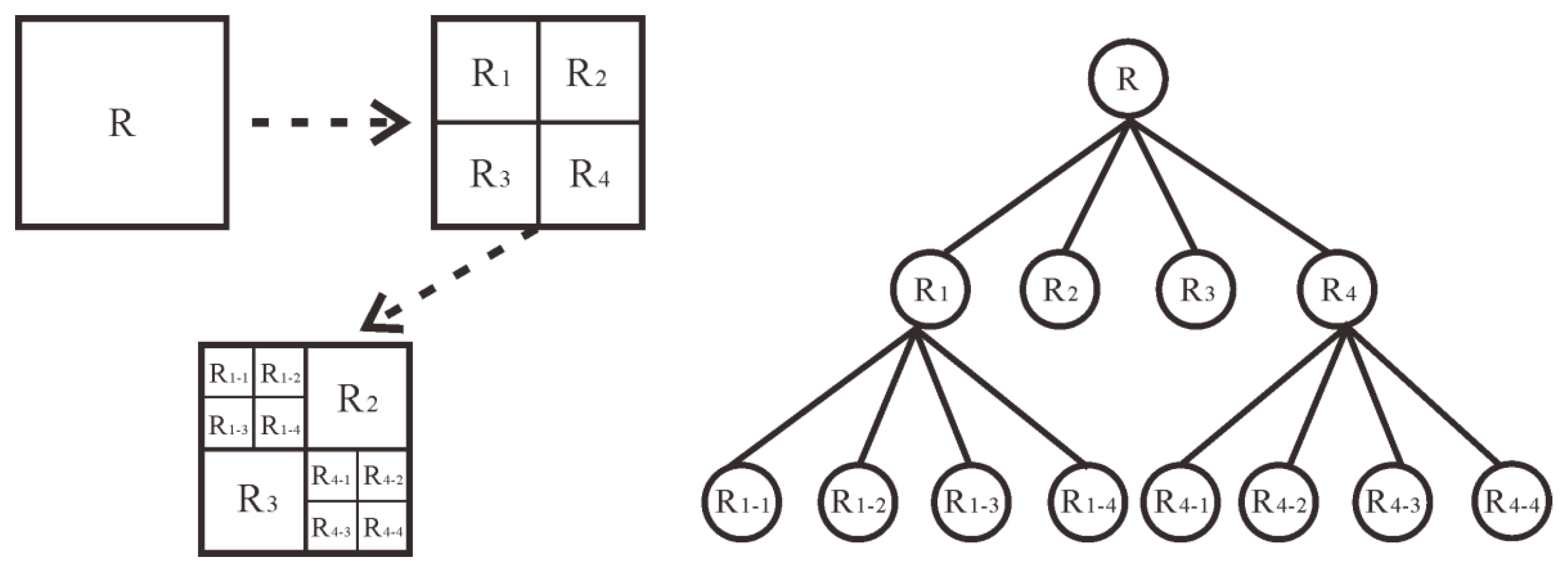
2.2. Adaptive Quadtree Data Compression Algorithm

Adaptive quadtree decomposition is an image segmentation algorithm based on uniformity detection. The segmentation scale of the data area with a large gradient change and uneven value is very small, so more data can be obtained, whereas the segmentation scale of the data region with a small gradient change and uniform value is coarse, so less data is obtained. Compared with the regular sampling method with equal intervals down-sampling, this method retains more detail and achieves the best approximation to the original data with the least amount of data.

Figure 1 shows the decomposition diagram of the three-level quadtree model. The quadtree decomposition algorithm is used to subdivide the two-dimensional space into four regions by recursion. The first level decomposition divides the region R into four sub-blocks R₁, R₂, R₃ and R₄. In the second decomposition, the region consistency of each sub-block is judged in turn. If R₂ and R₃ meet the regional consistency standard, they are no longer decomposed while if R₁ and R₂ do not meet the regional consistency criteria, they continue to be decomposed into four sub-blocks, namely, R_1–1, R_1–2, R_1–3, R_1–4 and R_4–1, R_4–2, R_4–3, R_4–4.

The uniformity of the data in the sub-blocks is called regional consistency. In this paper, the regional consistency standard is measured by variance, which is used to measure the magnitude and uniformity of fluctuations in the data. The larger the variance, the greater the difference in the data. Assuming that the amount of data in the segmented sub-block is n × n, the formula for calculating the variance is shown on the left side of Equation (9).

$$\frac{1}{n^2-1}{{\displaystyle {\sum }_{i,j=1,n}\left(f(i,j)-\overline{f}\right)}}^2<T$$

(10)

where $f(i,j)$ represents the value of the point $(i,j)$, $1\le i\le n$,$1\le j\le n$, and $\overline{f}$ represents the average value of the data in the sub-block. T is the variance threshold that is used to judge whether the sub-block is uniform. The variance threshold is not fixed, and the selection of threshold affects the error between the compressed data and the original data and the data compression ratio. When the variance threshold is large, it means that more data will be discarded, and the data error will increase and the compression ratio will decrease. By drawing a profile of error and threshold and a profile of the compression ratio and threshold, the intersection of the two sections can be selected as the best threshold.

Figure 2 shows a flowchart of the adaptive quadtree decomposition for data compression. First, given the segmentation size and variance threshold, when the sub-block size is larger than the minimum size and the variance T_i is greater than the given variance threshold T, the segmentation is continued until all the sub-blocks meet the conditions. In this way, the data from different sub-blocks of various sizes are obtained, and the average value and the coordinates of the center point are calculated, and are then stored as a compressed matrix. The method of using the average value of all data points of a sub-block to replace all of the points in the whole sub-block is called the mean method. It is essentially a low-pass filter that filters out the high-frequency part of the data for de-noising.

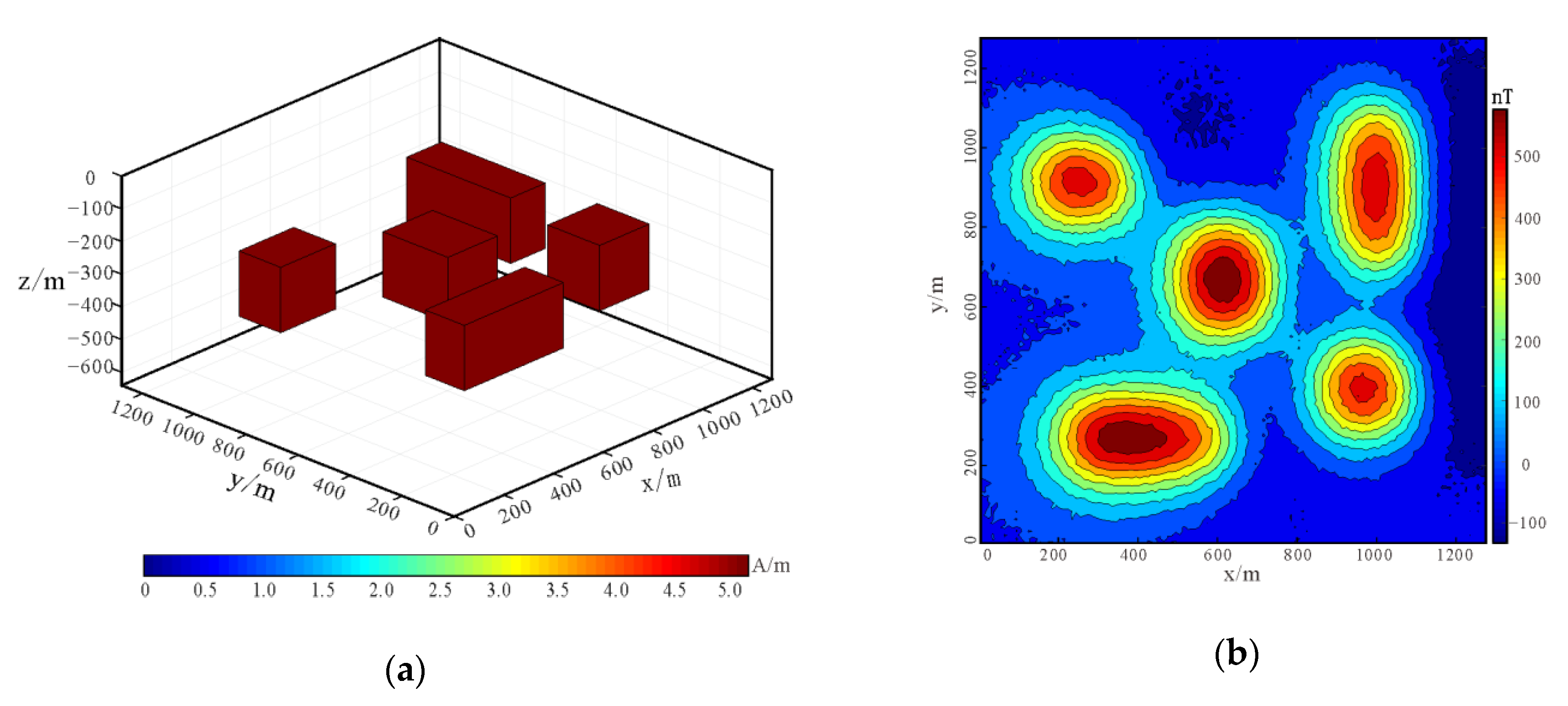
2.3. Synthetic Model Test

To illustrate the effectiveness and feasibility of data compression based on the adaptive quadtree decomposition algorithm in 3D magnetic inversion, two synthetic models are used in this paper.

Model 1: As shown in Figure 3a, the synthetic model is a simple cuboid with a length, width, and height of 400 m, 400 m, and 200 m, respectively, the buried depth of the top surface is 200 m, the magnetization is 5 A/m, the magnetic inclination is 60°, and the magnetic declination is 10°. Then, the forward calculation is carried out for the model. The observation height is set at 80 m, the survey network is 128 × 128, the spacing in x–axis and y–axis directions is 10 m, and the magnetic anomaly map with 7% Gaussian noise is added, as shown in Figure 3b.

The magnetic data for synthetic model 1 is compressed by the adaptive quadtree data compress algorithm. The parameter settings are as follows: the minimum grid is 4, the maximum grid is 16, and the variance threshold is 2000. Figure 4a,b show the cut image and the extracted data scatter map after data compression, respectively. The amount of data is reduced from 16384 points to 277 points. The compressed data is only 1.69% of the original data, and the error is 0.040.

Model 2: As shown in Figure 5a, the composite model is a complex model consisting of five different cubes. The depth of the buried surface is 200 m, and the magnetization is 5 A/m. The inclination angle and magnetic declination angle are the same as those of model 1. The magnetic anomaly map with 7% Gaussian noise is shown in Figure 5b. The magnetic data for synthetic model 2 is compressed by adaptive quadtree decomposition algorithm. The parameter settings are as follows: the minimum grid is 4, the maximum grid is 16, and the variance threshold is 1600. Figure 6a shows the cut image using quadtree decomposition algorithm, and Figure 6b shows the compression algorithm extracts data scatter diagram, the data volume is reduced from 16384 points to 505 points, thus the compressed data volume is only 3.08% of the original data, and the error is 0.067.

As can be seen from Figure 4b and Figure 6b, the data points at the anomaly boundary are intensively sampled, which fully preserves the detailed features while only a small number of data points are reserved at the places where the anomaly changes slowly, thus greatly reducing the magnitude of the data. The compressed data are reconstructed as shown in Figure 4c and Figure 6c. The results show that the compressed data retains the abnormal details and effectively eliminates the noise compared with the original data.

Taking the inversion calculation of model 2 as an example, we can compare the inversion using the compressed data and the inversion using the original data. The underground grid is divided into 64 × 64 × 32, and the grid spacing is 20 m × 20 m × 20 m. The horizontal and vertical slices of the inversion results are shown in Figure 7. When comparing the inversion results of the compressed data with the original data, it can be seen that the resolution of the compressed data is better than that of the original data. The results show that although some information is lost after data compression, the detailed features of the data are still retained. Since the step length and direction are calculated from all the data in the inversion iteration, when the inefficient information is reduced, the effective information is given more weight, which improves the efficiency of the iteration and makes the resolution of the anomaly boundary higher than the other locations, makes the inversion results more convergent, and can also show smaller anomalies.

3. Application in Mineral Exploration

The adaptive quadtree compression algorithm was applied to the magnetic data set collected for the Ma’anshan magnetite deposit. The magnetite deposit is located in the Ningwu mining area in the middle and lower reaches of the Yangtze River. The magmatic activity in this area was a strong, mainly volcanic eruption and magmatic intrusion in the Yanshanian period. The main subvolcanic rock body in the survey area is diorite porphyrite, which is the mineralization mother rock of iron and sulfur deposits in the mining area. Diorite porphyrite with its medium magnetism and magnetite with high magnetism have an obvious magnetic difference from the surrounding rocks, which are the basis of magnetic exploration. There are many sulfur and iron ore mining points in this area (see Figure 8). To find ore in the periphery and deep part of the old mine, the Unmanned Aerial Vehicle (UAV) aeromagnetic survey system was used to investigate this area. The total survey line length is 111.9 km, the average flight height is 84 m, the line distance is 100 m, and the average point distance is 0.86 m. A total of 145495 data points were collected. After data preprocessing and IGRF International Geomagnetic Reference Field (IGRF) correction, the minimum curvature gridding was carried out with a grid size of 25 m. Finally, the contour map of the total magnetic anomaly obtained is shown in Figure 8a, and the amplitude of anomaly is −1800 nT–3400 nT. The total magnetic field data is the superposition effect of different magnetic geological bodies. To separate the local field from the background field, the upward continuation method was used. Upward continuation was used to calculate the abnormal value of a certain height above the observation plane according to the measured anomaly [46,47]. Since the potential field value is inversely proportional to the square of the distance from the field source to the observation point, the field value of the field source with different depths has different changes in speed when the same height is extended. When the upward continuation is performed, the field source with large depth is highlighted because of its slow attenuation speed, thus the deep anomaly can be highlighted. In the upward continuation of the data, when the continuation height is greater than 300 m, the field change is very small, which can be approximately regarded as the regional magnetic field. As shown in Figure 8b, the residual gravity anomaly can be separated by subtracting the upward continuation anomaly from the total magnetic anomaly. There are two main North-East (N-E) trending high magnetic anomaly belts, in which there are many elliptical and equiaxed local anomalies with large amplitude variations. Some of the local anomalies correspond to the known iron deposits in the area.

To restore the distribution of magnetic field sources, the underground was divided into 64 × 64 × 20 grids, each with a length of 50 m. Firstly, the adaptive quadtree decomposition method was used to compress the magnetic data, and the variance threshold was set to 7800 (see Figure 9). The location map of the sampling points is shown in Figure 10. The black cross in the graph represents the position of the sampling data, with 1534 sampling points, accounting for 1.05% of the original data. The compressed data were used for 3D magnetic inversion, and the inversion results are shown in Figure 11.

A total of 10 medium and high magnetization anomalies were obtained by 3D inversion, and were labeled M1-M10. The spatial location map is shown in Figure 11a. Figure 11b shows the inversion results at different depths. The distribution of anomalies corresponds to the surface magnetic anomalies, and their buried depth is between 100 m and 500 m. Figure 11c–f show the location characteristics of ore bodies at different sections. Combining existing geological data and inversion results, the M1 anomaly was located in the Xiang Shan (XS) pyrite area, which is a mined-out area above 100 m underground. The inversion results show that there are magnetite ore bodies under the mined-out area, inclined to the southeast with a deepest depth of 500 m. The M2 anomalous body is located in the south of the Nan Shan (NS) iron mining pit. A large number of diorite porphyrite, magnetite orebody, and pyrite ore body are exposed on the surface. It is speculated that the magnetite (mineralized) body exists underground at a buried depth of 200–400 m. Diorite porphyry and magnetite ore bodies are exposed on the surface where the M3 anomaly is located. Ao Shan (AS) iron ore is located near the southeast side. It is speculated that the anomaly is a magnetized ore body. M4 anomaly body is located on the north side of the AS iron ore pit. The exposed stratum is the Lower Cretaceous, and the residual magnetization is large. It is presumed to be a magnetized mineralized body. The buried depth is about 100 m, the thickness is about 400 m, and the width is more than 300 m. The M5 anomalous body is located in the Luo Bo Shan (LBS) mining area. The magnetite at the top of the location has been mined. There is magnetite in the deep rock body at a depth of more than 300 m, and the thickness is less than 100 m. The M8 anomaly shows obvious high magnetization, and it is speculated that there are magnetite ore bodies in the lower part. The anomalous bodies (M6, M7, M9, M10) in the northeast and southeast of the survey area have low magnetization and are presumed to be diorite porphyrite. Therefore, there are five magnetite bodies, M1, M2, M3, M4, and M8 in this area, which are large in scale and they have potential for development.

4. Conclusions

In this paper, an adaptive quadtree decomposition method is proposed to compress magnetic data, which is decomposed recursively until the data in each quadrant meets the regional consistency standard. The model tests show that the method can be used for fine sampling where the gradient of magnetic anomaly data is large, and for sparse sampling at the place with a gentle anomaly change, to realize the effective compression of magnetic data and greatly improve the calculation efficiency of 3D inversion. In addition, the mean method can suppress noise and improve the resolution of inversion results.

The method was applied to the magnetic data for the Ma’anshan mining area, and five possible areas of magnetite orebodies were delineated in the surrounding and deep part of the existing mining area, which provides some significant guidance for the next prospecting work.

The 3D magnetic inversion algorithm is an important means of data interpretation. However, the calculation efficiency is very low. The adaptive quadtree decomposition calculation is only used to compress the data space. When the amount of data is large, the underground subdivision grid is very large, which still leads to the calculation speed being very slow. The calculation efficiency can be further improved by combining wavelet compression technology, adaptive mesh generation technology, parallel computing, and so on.

References

1. Nabighian, M.N.; Hansen, R.O.; Lafehr, T.R.; Li, Y.; Peirce, J.W.; Phillips, J.D.; Ruder, M.E. The historical development of the magnetic method in exploration. Geophysics 2005, 70, 33ND–61ND. [Google Scholar] [CrossRef]
2. Yan, H.-F.; Liu, G.-F. A extension of probability tomography of gravity data. Prog. Geophys. 2014, 29, 1837–1842. [Google Scholar]
3. Mauriello, P.; Patella, D. Localization of magnetic sources underground by a data adaptive tomographic scanner. arXiv 2005, arXiv:0511192v2. [Google Scholar]
4. Mauriello, P.; Patella, D. Localization of magnetic sources underground by a probability tomography approach. Prog. Electromagn. Res. M 2008, 3, 27–56. [Google Scholar] [CrossRef] [Green Version]
5. Guo, L.; Shi, L.; Meng, X. 3D correlation imaging of magnetic total field anomaly and its vertical gradient. J. Geophys. Eng. 2011, 8, 287–293. [Google Scholar] [CrossRef] [Green Version]
6. Boschetti, F.; Dentith, M.; List, R. Inversion of potential field data by genetic algorithms. Geophys. Prospect. 1997, 45, 461–478. [Google Scholar] [CrossRef]
7. Guan, Z.-N.; Hou, J.-S.; Huang, L.-P.; Yao, C.-L. Inversion of gravity and magnetic anomalies using pseduo-BP neural network method and its application. Chin. J. Geophys. 1998, 41, 242–251. [Google Scholar]
8. Pilkington, M. 3-D magnetic imaging using conjugate gradients. Geophysics 1997, 62, 1132–1142. [Google Scholar] [CrossRef]
9. Li, Y.; Melo, A.; Martinez, C.; Sun, J. Geology differentiation: A new frontier in quantitative geophysical interpretation in mineral exploration. Lead. Edge 2019, 38, 60–66. [Google Scholar] [CrossRef]
10. Zhdanov, M.S.; Alfouzan, F.; Cox, L.H.; Alotaibi, A.M.; Alyousif, M.M.; Sunwall, D.; Endo, M. Large-Scale 3D Modeling and Inversion of Multiphysics Airborne Geophysical Data: A Case Study from the Arabian Shield, Saudi Arabia. Minerals 2018, 8, 271. [Google Scholar] [CrossRef] [Green Version]
11. Green, W.R. Inversion of Gravity Profiles by Use of a Backus-Gilbert Approach. Geophysics 1975, 40, 763–772. [Google Scholar] [CrossRef]
12. Last, B.J.; Kubik, K. Compact gravity inversion. Geophysics 1983, 48, 713–721. [Google Scholar] [CrossRef]
13. Li, Y.; Oldenburg, D.W. 3-D inversion of magnetic data. Geophysics 1996, 61, 394–408. [Google Scholar] [CrossRef]
14. Li, Y.; Oldenburg, D.W. 3-D inversion of gravity data. Geophysics 1998, 63, 109–119. [Google Scholar] [CrossRef]
15. Portniaguine, O.; Zhdanov, M.S. 3-D magnetic inversion with data compression and image focusing. Geophysics 2000, 67, 1532–1541. [Google Scholar] [CrossRef] [Green Version]
16. Portniaguine, O. Image Focusing and Data Compression in the Solution of Geophysical Inverse Problems. Ph.D. Thesis, The University of Utah, Salt Lake City, UT, USA, 1999. [Google Scholar]
17. Zhdanov, M.S.; Ellis, R.G.; Mukherjee, S. Three-dimensional regularized focusing inversion of gravity gradient tensor component data. Geophysics 2004, 69, 925–937. [Google Scholar] [CrossRef]
18. Sun, J.; Li, Y. Geophysical inversion using petrophysical constraints with application to lithology differentiation. In Proceedings of the 2011 SEG Annual Meeting, San Antonio, TX, USA, 18–23 September 2011. [Google Scholar]
19. Sun, J.; Li, Y. Multidomain petrophysically constrained inversion and geology differentiation using guided fuzzy c-means clustering. Geophysics 2015, 80, ID1–ID18. [Google Scholar] [CrossRef]
20. Silva, J.B.C.; Medeiros, W.E.; Barbosa, V.C.F. Potential-field inversion: Choosing the appropriate technique to solve a geologic problem. Geophysics 2001, 66, 511–520. [Google Scholar] [CrossRef]
21. Pilkington, M. 3D magnetic data-space inversion with sparseness constraints. Geophysics 2008, 74, L7–L15. [Google Scholar] [CrossRef]
22. Commer, M. Three-dimensional gravity modeling and focusing inversion using rectangular meshes. Geophys. Prospect. 2011, 59, 966–979. [Google Scholar]
23. Paoletti, V.; Ialongo, S.; Florio, G.; Fedi, M.; Cella, F. Self-constrained inversion of potential fields. Geophys. J. Int. 2013, 195, 854–869. [Google Scholar] [CrossRef] [Green Version]
24. Sun, J.; Li, Y. Adaptive Lp inversion for simultaneous recovery of both blocky and smooth features in a geophysical model. Geophys. J. Int. 2014, 197, 882–899. [Google Scholar] [CrossRef] [Green Version]
25. Uieda, L.; Barbosa, V.C.F. Robust 3D gravity gradient inversion by planting anomalous densities. Geophysics 2012, 77, G55–G66. [Google Scholar] [CrossRef]
26. Li, Y.; Oldenburg, D.W. Fast inversion of large-scale magnetic data using wavelet transforms and a logarithmic barrier method. Geophys. J. Int. 2003, 152, 251–265. [Google Scholar] [CrossRef] [Green Version]
27. Yao, C.; Hao, T.; Guan, Z.; Zhang, J. High-speed calculation and effective storage method and technology in 3D inversion of gravity and magnetic genetic algorithm. Chin. J. Geophys. 2003, 46, 252–258. [Google Scholar] [CrossRef]
28. Cuma, M.; Wilson, G.A.; Zhdanov, M.S. Large-scale 3D inversion of potential field data. Geophys. Prospect. 2012, 60, 1186–1199. [Google Scholar] [CrossRef]
29. Čuma, M.; Zhdanov, M.S. Massively parallel regularized 3D inversion of potential fields on CPUs and GPUs. Comput. Geoences 2014, 62, 80–87. [Google Scholar] [CrossRef]
30. Hou, Z.; Huang, D. Multi-GPU parallel algorithm design and analysis for improved inversion of probability tomography with gravity gradiometry data. J. Appl. Geophys. 2017, 144, 18–27. [Google Scholar] [CrossRef]
31. Ascher, U.M.; Haber, E. Grid refinement and scaling for distributed parameter estimation problems. Inverse Probl. 2001, 17, 571–590. [Google Scholar] [CrossRef] [Green Version]
32. Davis, K.; Li, Y. Fast solution of geophysical inversion using adaptive mesh, space-filling curves and wavelet compression. Geophys. J. Int. 2011, 185, 157–166. [Google Scholar] [CrossRef] [Green Version]
33. Davis, K.; Li, Y. Efficient 3D inversion of magnetic data via octree-mesh discretization, space-filling curves, and wavelets. Geophys. J. Soc. Explor. Geophys. 2013, 78, J61–J73. [Google Scholar] [CrossRef]
34. Yang, M.; Wang, W.; Welford, J.K.; Farquharson, C. 3D gravity inversion with optimized mesh based on edge and center anomaly detection. Geophysics 2019, 84, 1–62. [Google Scholar] [CrossRef]
35. Foks, N.L.; Krahenbuhl, R.; Li, Y. Adaptive sampling of potential-field data: A direct approach to compressive inversion. Geophysics 2014, 79, 1–9. [Google Scholar] [CrossRef]
36. Vatankhah, S.; Renaut, R.A.; Ardestani, V.E. Total variation regularization of the 3-D gravity inverse problem using a randomized generalized singular value decomposition. Geophys. J. Int. 2018, 213, 695–705. [Google Scholar] [CrossRef] [Green Version]
37. Toushmalani, R.; Saibi, H. Fast 3D inversion of gravity data using Lanczos bidiagonalization method. Arab. J. Geosci. 2015, 8, 4969–4981. [Google Scholar] [CrossRef]
38. Meng, Z.; Li, F.; Zhang, D.; Xu, X.; Huang, D. Fast 3D inversion of airborne gravity-gradiometry data using Lanczos bidiagonalization method. J. Appl. Geophys. 2016, 132, 211–228. [Google Scholar] [CrossRef]
39. Rezaie, M.; Moradzadeh, A.; Kalate, A.N.; Aghajani, H. Fast 3D Focusing Inversion of Gravity Data Using Reweighted Regularized Lanczos Bidiagonalization Method. Pure Appl. Geophys. 2017, 174, 359–374. [Google Scholar] [CrossRef]
40. Klinger, A.; Dyer, C.R. Experiments on Picture Representation Using Regular Decomposition. Comput. Graph. Image Process. 1976, 5, 68–105. [Google Scholar] [CrossRef]
41. Yerry, M.A.; Shephard, M.S. A Modified Quadtree Approach To Finite Element Mesh Generation. IEEE Comput. Graph. Appl. 1983, 3, 39–46. [Google Scholar] [CrossRef]
42. Jackson, D.J.; Mahmoud, W.; Stapleton, W.A.; Gaughan, P.T. Faster fractal image compression using quadtree recomposition. Image Vis. Comput. 1997, 15, 759–767. [Google Scholar] [CrossRef]
43. Zeng, Z.; Cumming, I. SAR image data compression using a tree-structured wavelet transform. IEEE Trans. Geosci. Remote Sens. 2001, 39, 546–552. [Google Scholar] [CrossRef] [Green Version]
44. Tikhonov, A.N.; Arsenin, V.Y. Solutions of ill-posed problems. Math. Comput. 1977, 32, 491. [Google Scholar]
45. Li, Y. 3-D Inversion of gravity gradiometer data. In Proceedings of the SEG Int’l Exposition and Annual Meeting, San Antonio, TX, USA, 9–14 September 2001. [Google Scholar]
46. Bertrand, L.; Gavazzi, B.; Mercier de Lépinay, J.; Diraison, M.; Géraud, Y.; Munschy, M. On the Use of Aeromagnetism for Geological Interpretation: 2. A Case Study on Structural and Lithological Features in the Northern Vosges. J. Geophys. Res. Solid Earth 2020, 125, 5. [Google Scholar] [CrossRef]
47. Pilkington, M.; Boulanger, O. Potential field continuation between arbitrary surfaces—Comparing methods. Geophysics 2017, 82, J9–J25. [Google Scholar] [CrossRef]
Figure 1. A three-level quadtree decomposition diagram.
Applsci 10 07636 g001
Figure 2. The flowchart for the adaptive quadtree decomposition.
Applsci 10 07636 g002
Figure 3. Synthetic model 1: (a) schematic diagram; (b) magnetic anomaly contour map.
Applsci 10 07636 g003
Figure 4. Synthetic model 1: (a) the image is segmented by quadtree; (b) the scattered point location map of data extracted by compression algorithm; (c) contour map of magnetic anomalies reconstructed from compressed data.
Applsci 10 07636 g004
Figure 5. Synthetic model 2: (a) schematic diagram; (b) magnetic anomaly contour map.
Applsci 10 07636 g005
Figure 6. Synthetic model 2: (a) the image is segmented by quadtree; (b) the scattered point location map of data extracted by compression algorithm; (c) contour map of magnetic anomalies reconstructed from compressed data.
Applsci 10 07636 g006
Figure 7. Inversion results for model 2: (ac) are the inversion results of the compressed data in the slice of z = 300 m, x = 1000 m, and y = 1000 m, respectively. (df) are the inversion results for the original data in the slice of z = 300 m, x = 1000 m, and y = 1000 m, respectively. The white line represents the model.
Applsci 10 07636 g007
Figure 8. (a) Contour map of the original magnetic anomaly; (b) contour map of the local magnetic anomaly. The symbol with a cross in the circle indicates the location of the existing mining points.
Applsci 10 07636 g008
Figure 9. Reconstruction error and compression ratio change with a threshold. The intersection of the two lines was selected as the final threshold.
Applsci 10 07636 g009
Figure 10. The scattered point location map of data extracted by the compression algorithm for the Ma’anshan region. The black cross represents the position of the sampling data.
Applsci 10 07636 g010
Figure 11. Inversion results: (a) spatial distribution of the 3D inversion results; (b) the inversion results at different depths; (cf) show the distribution characteristics of ore bodies in the profile x = 900 m, x = 1200 m, x = 1800 m, and x = 2200 m, respectively.
Applsci 10 07636 g011
Publisher’s Note: MDPI stays neutral with regard to jurisdictional claims in published maps and institutional affiliations.