On the Adoption of Global/Local Approaches for the Thermomechanical Analysis and Design of Liquid Rocket Engines


Abstract
:1. Introduction
2. Mathematical Model
2.1. Heat Conduction Model
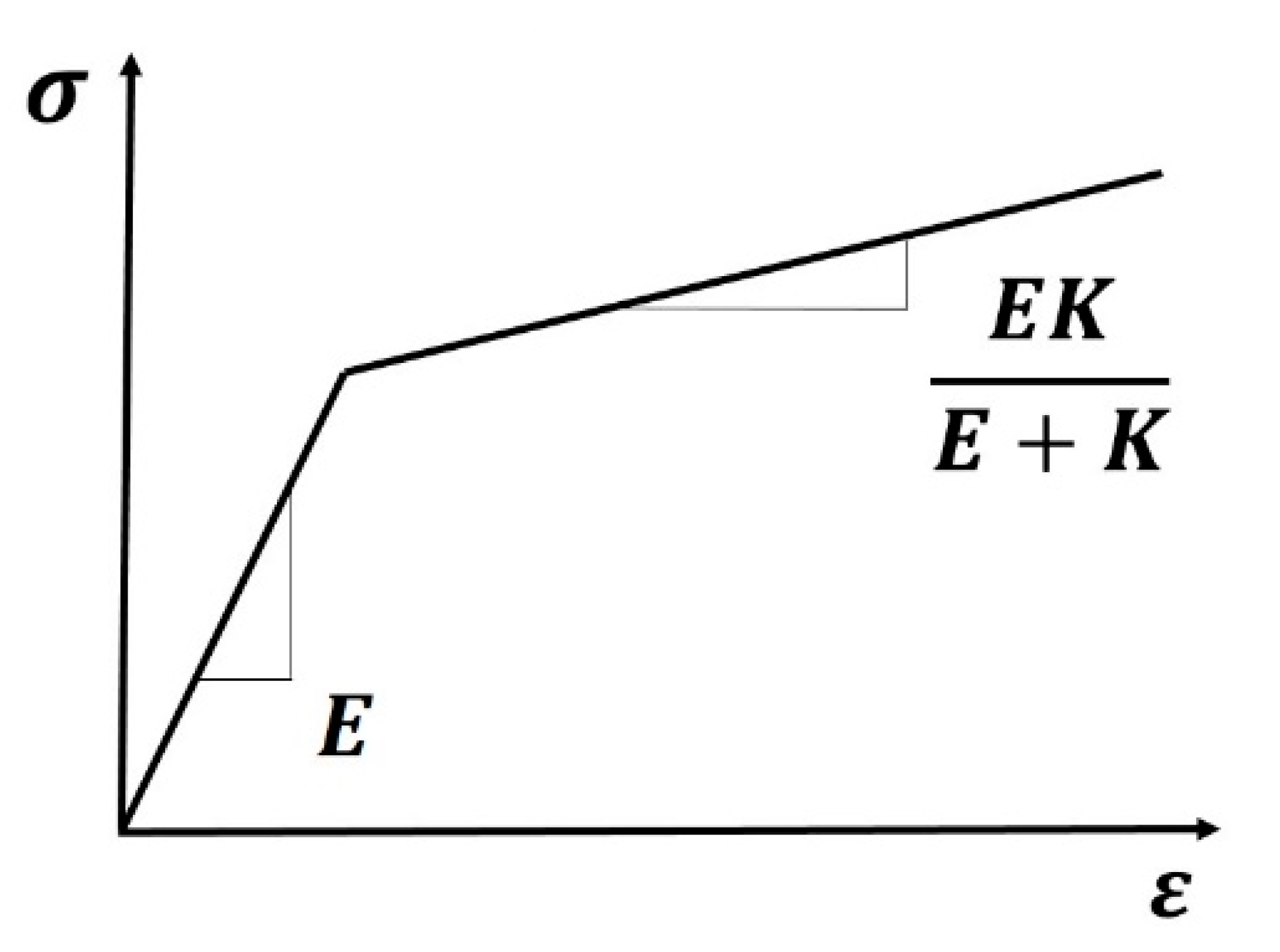
2.2. Structural Model
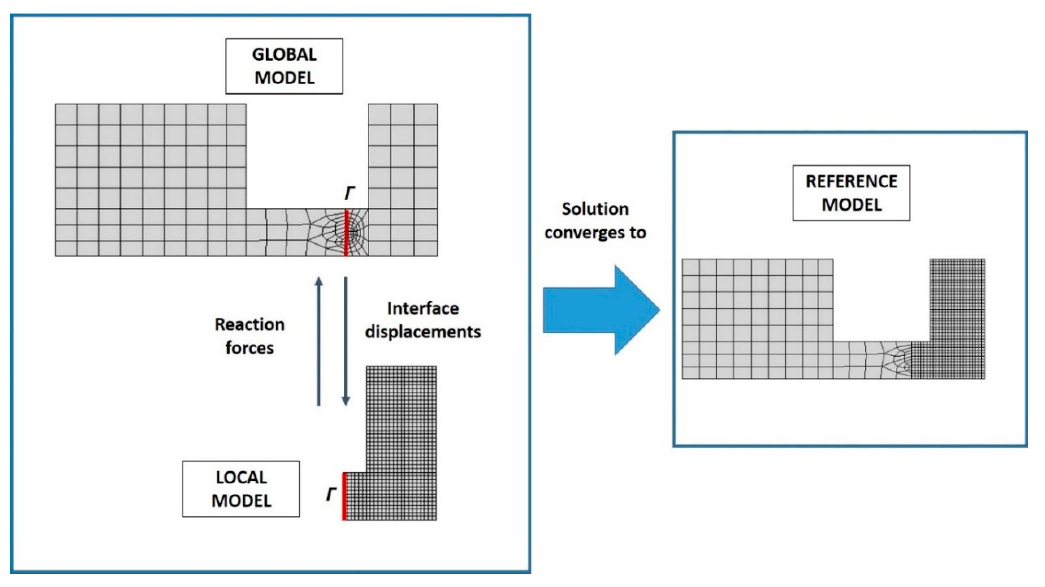
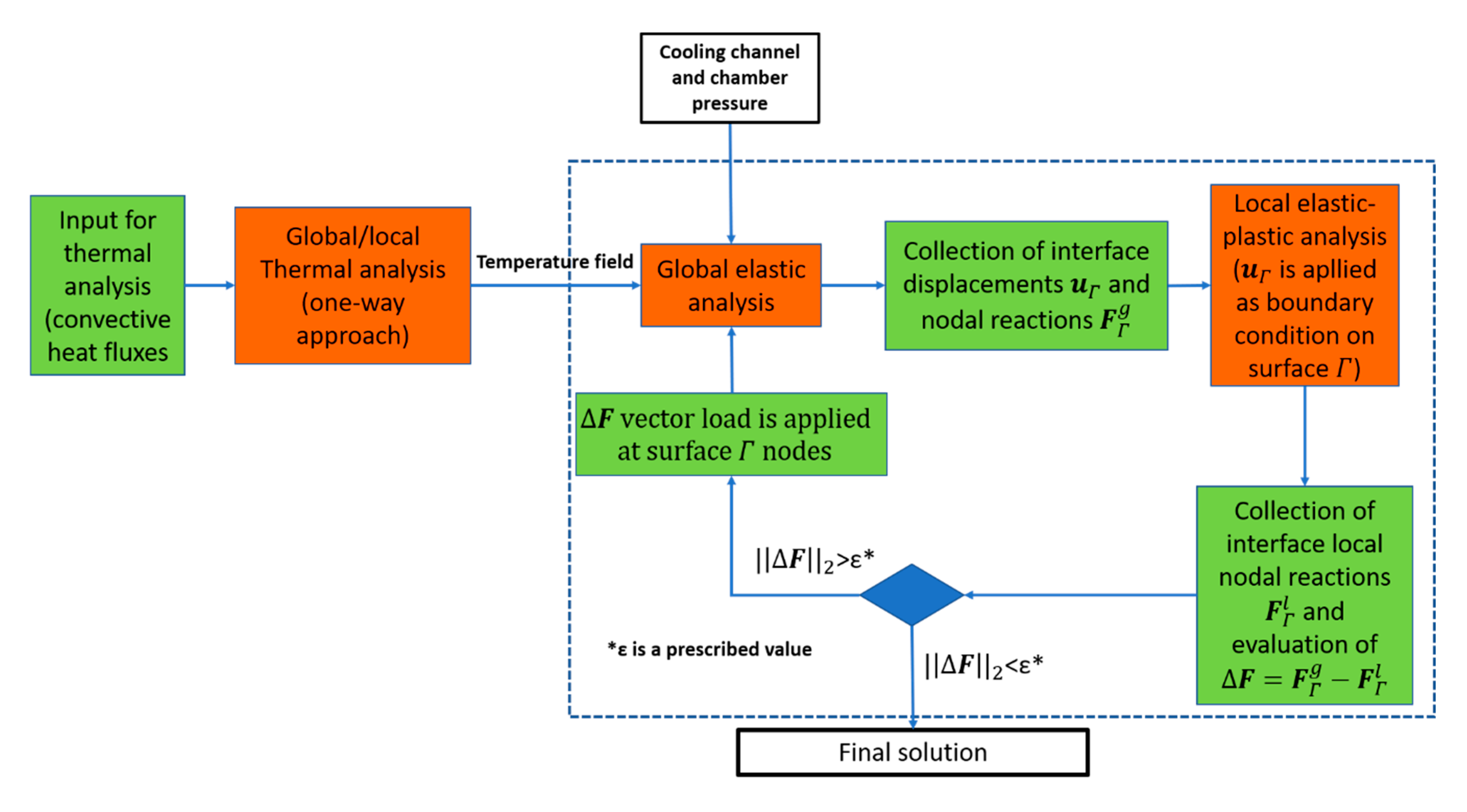
3. Iterative Coupling Algorithm
- Global Model—it is a global elastic model with a coarse mesh;
- Local Model—it is a submodel with a fine mesh in which elastic–plastic behavior is considered;
- Reference Model—it is a nonlinear model in which the discretization corresponds to that of the Local Model in the submodelled domain and to that of the Global Model in the remaining part of the domain.
- a global elastic analysis is performed on the Global model with a coarse mesh,
- the interface displacements and nodal forces are collected ( is the interface curve),
- a local nonlinear analysis is performed on the submodel applying as boundary conditions at the interface (external boundary for the submodel),
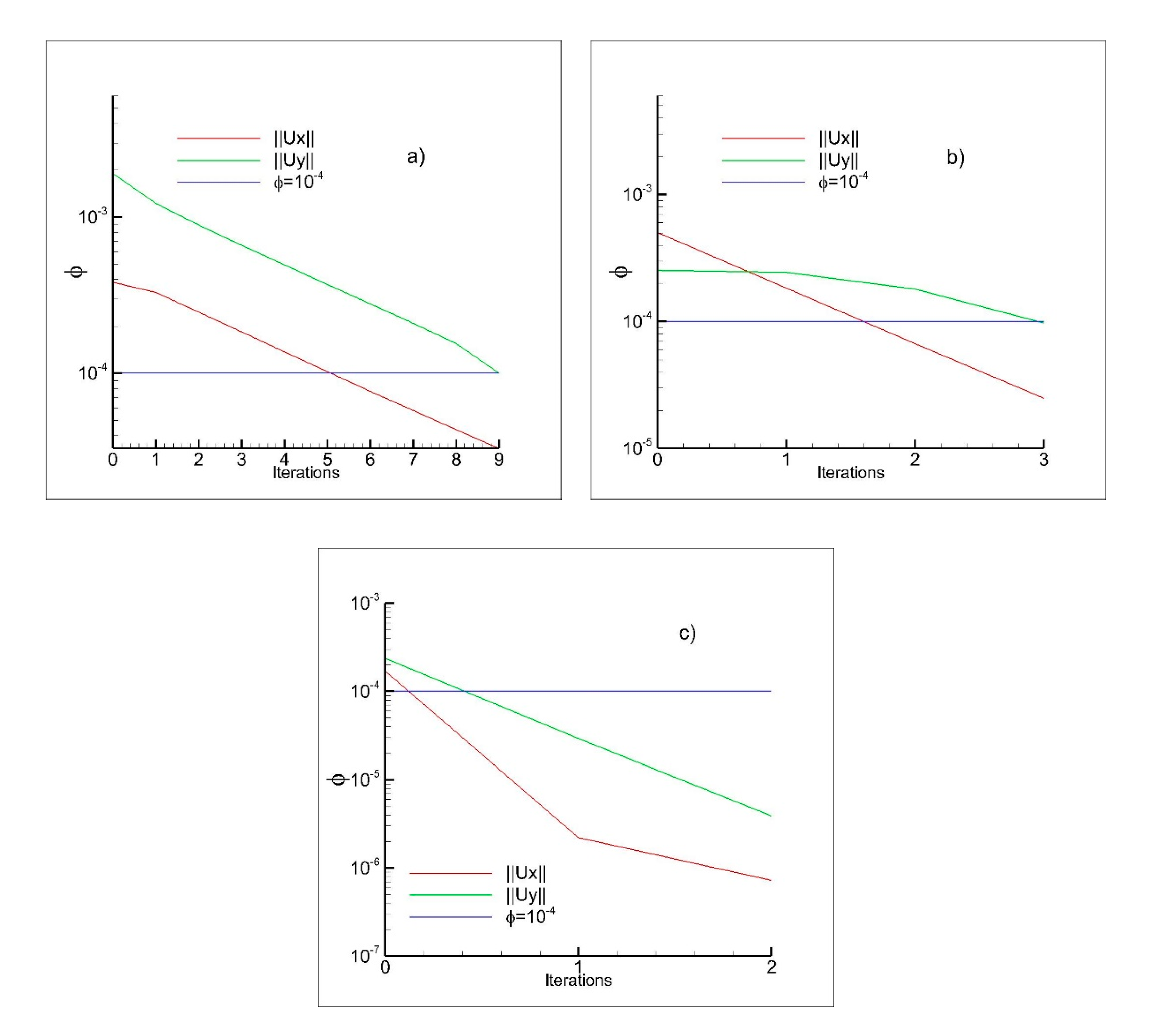
- nodal forces , evaluated by the local analysis, are collected and subtracted from obtaining ,
- if is greater than a prescribed limit Ɛ, then the process comes back to step 1 where is applied to the Global model at the interface ,
- if is lower than a prescribed limit Ɛ, the final solution is identified,
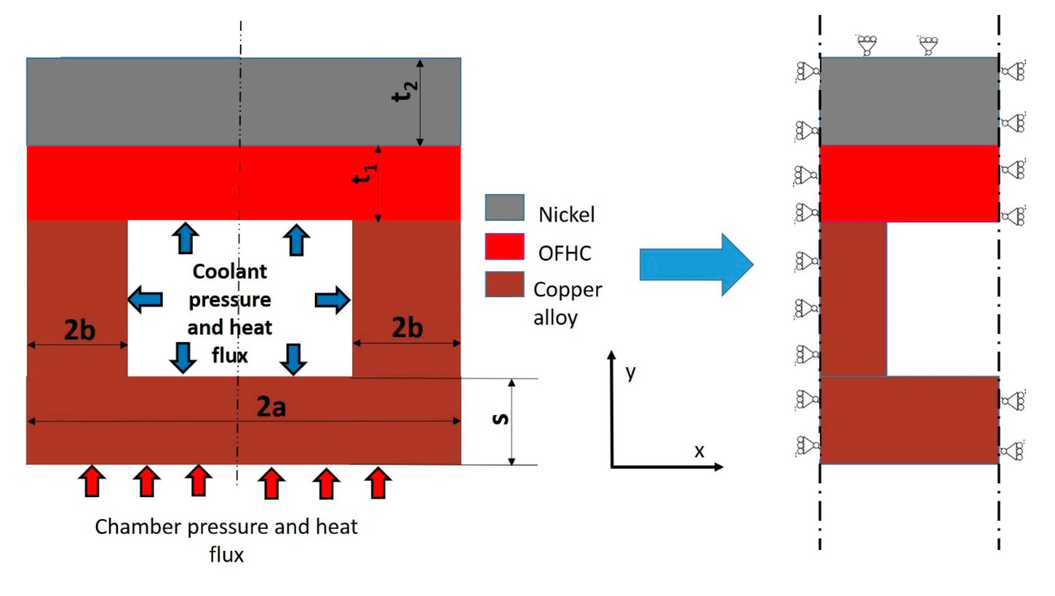
4. Numerical Model
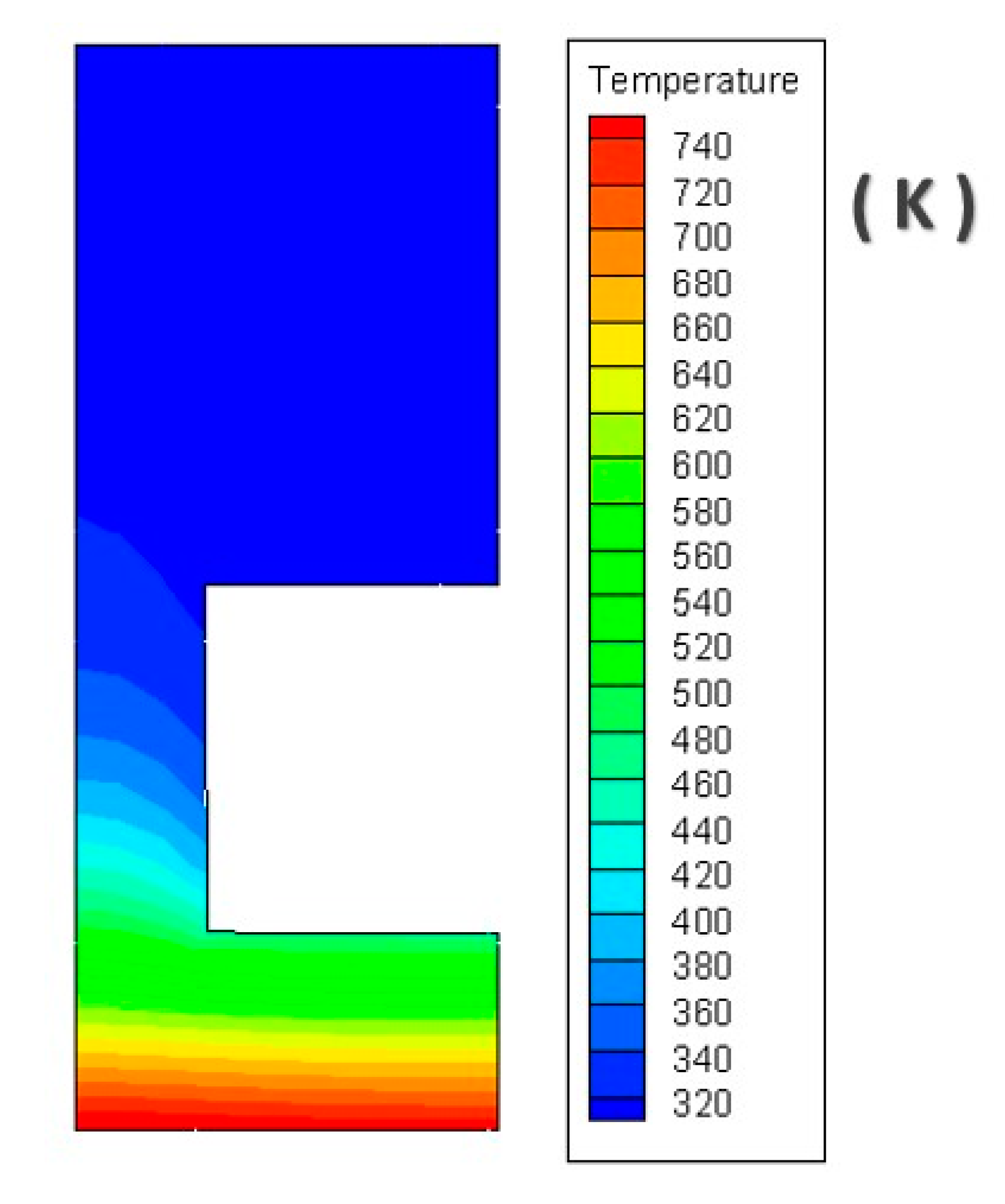
- One-way coupling between the thermal and the structural problem, namely, the temperature field, evaluated by the thermal analysis, is applied as body loads for the structural nonlinear analysis. On the other hand, since for this kind of problem the displacement/strain field does not have a significant impact on the temperature field, as demonstrated in several works [33], the thermal analysis is not repeated.
- Small deformations, that is, a geometrical linear model is adopted.
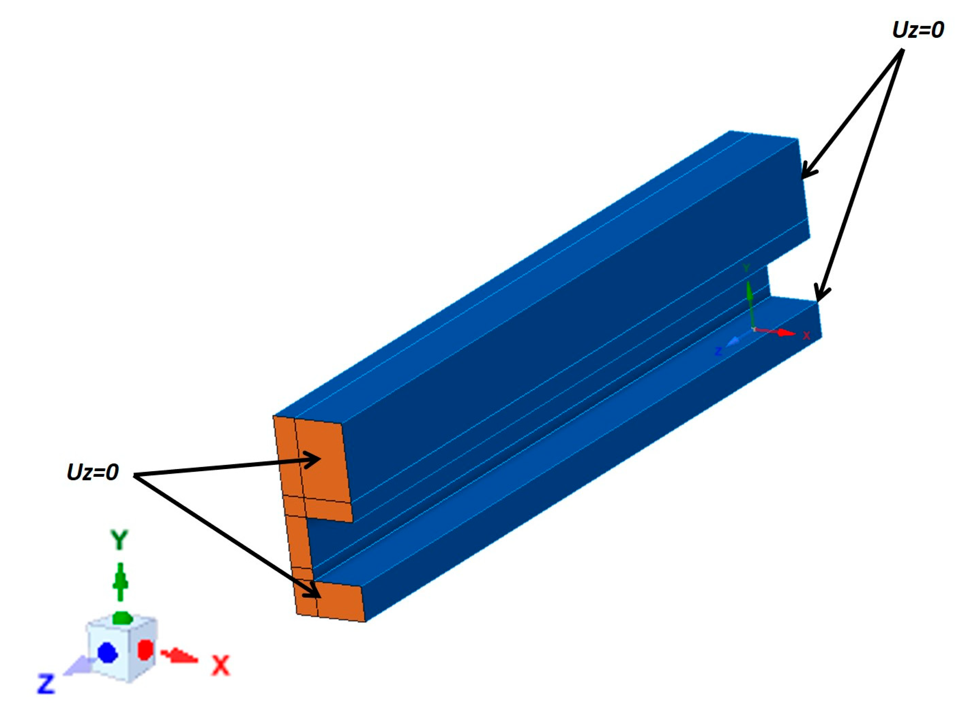
4.1. Boundary Conditions
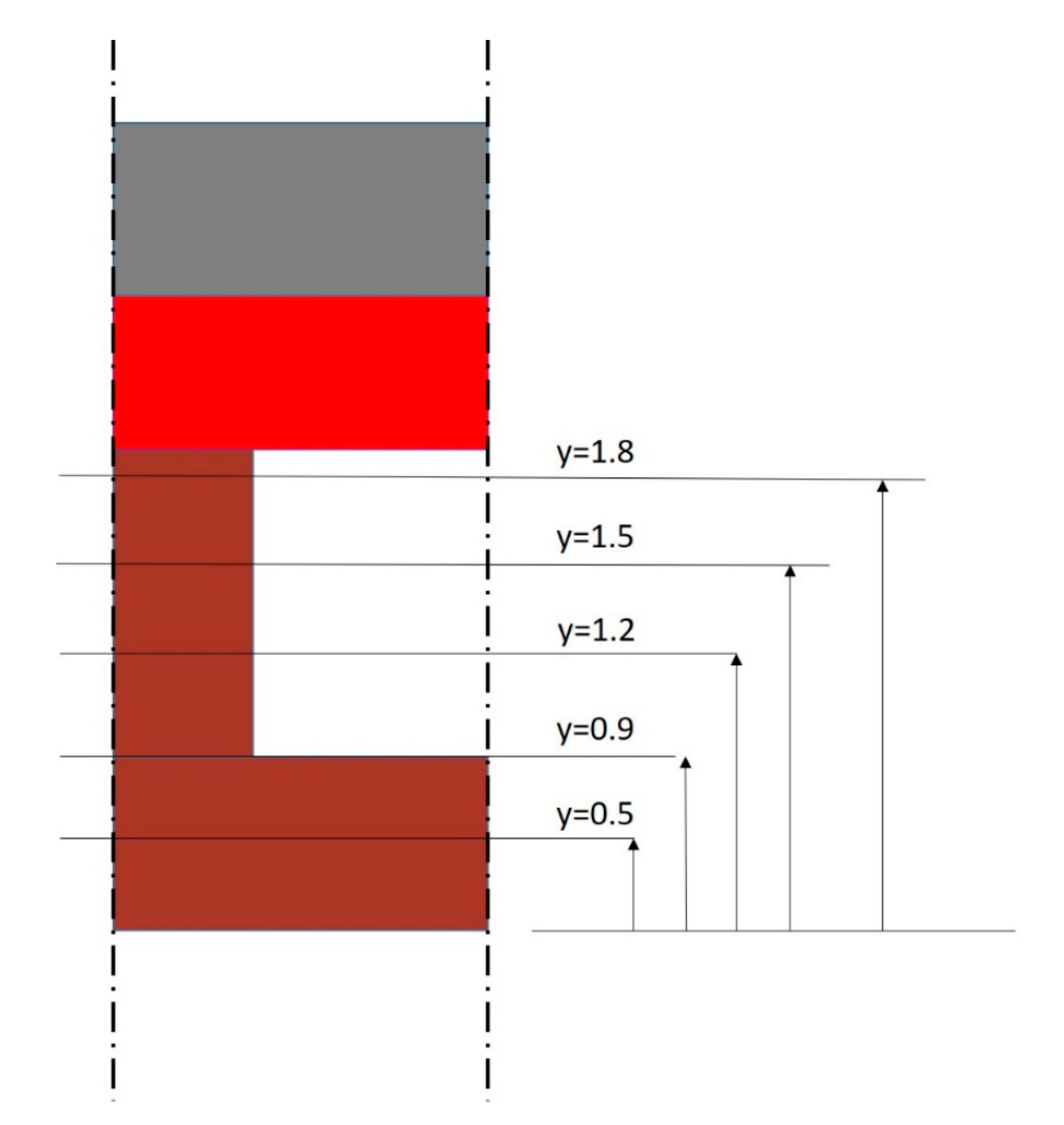
- Local Model 1—extends between y = 0 and y = 0.5, in such a way that the interface with the Global Model occurs in an area where plastic strains are expected;
- Local Model 2—with the interface placed in correspondence of what presumably is the limit between linear (elastic behavior) and nonlinear (elastic–plastic behavior) areas;
- Local Model 3—such that the interface occurs where no plastic strains are envisaged;
- Local Model 4—extends between y = 0 and y = 1.5;
- Local Model 5—extends between y = 0 and y = 1.8.
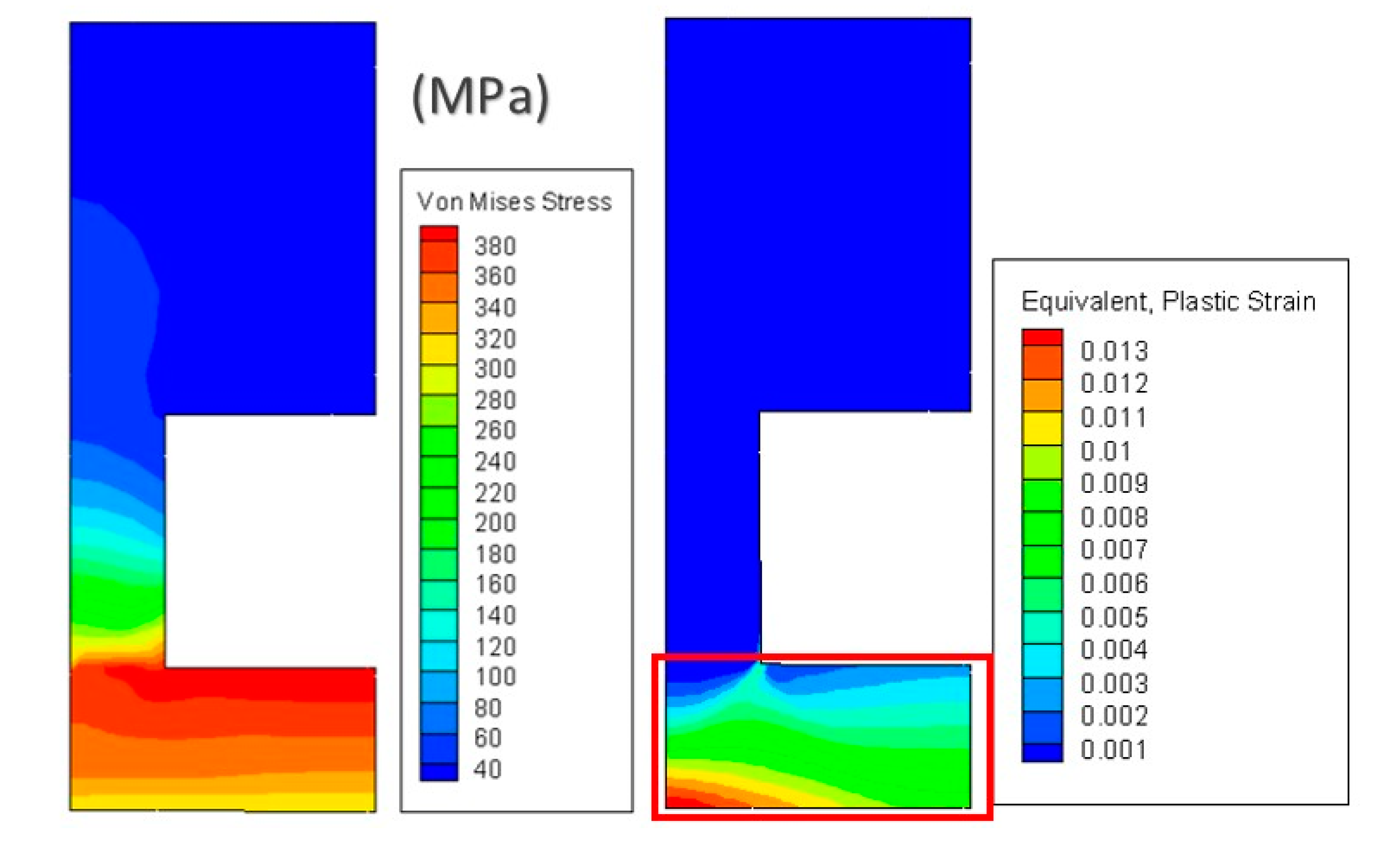
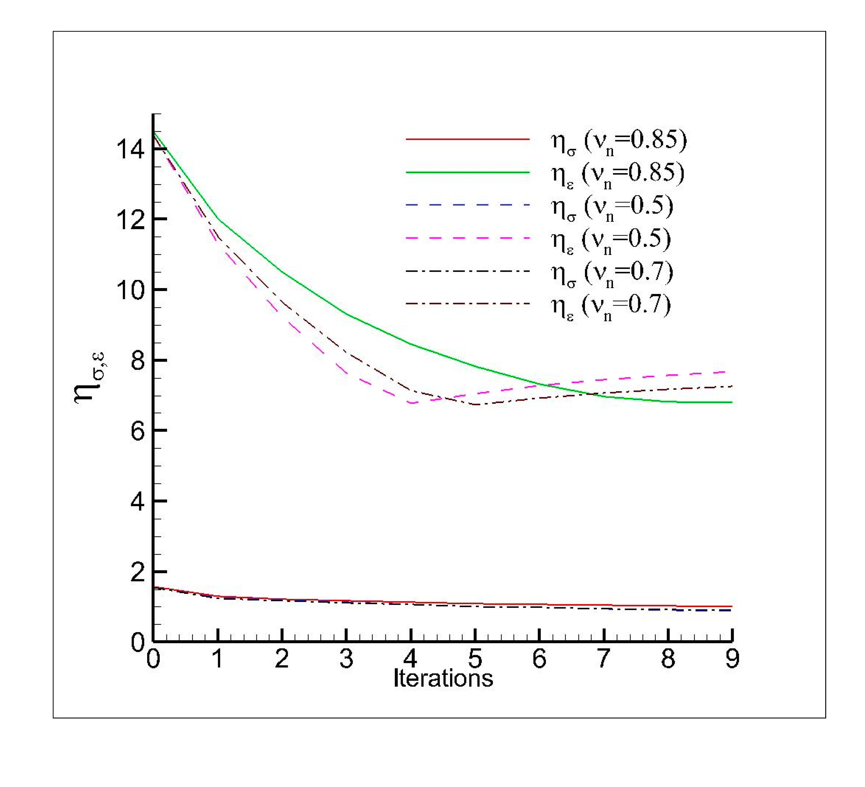
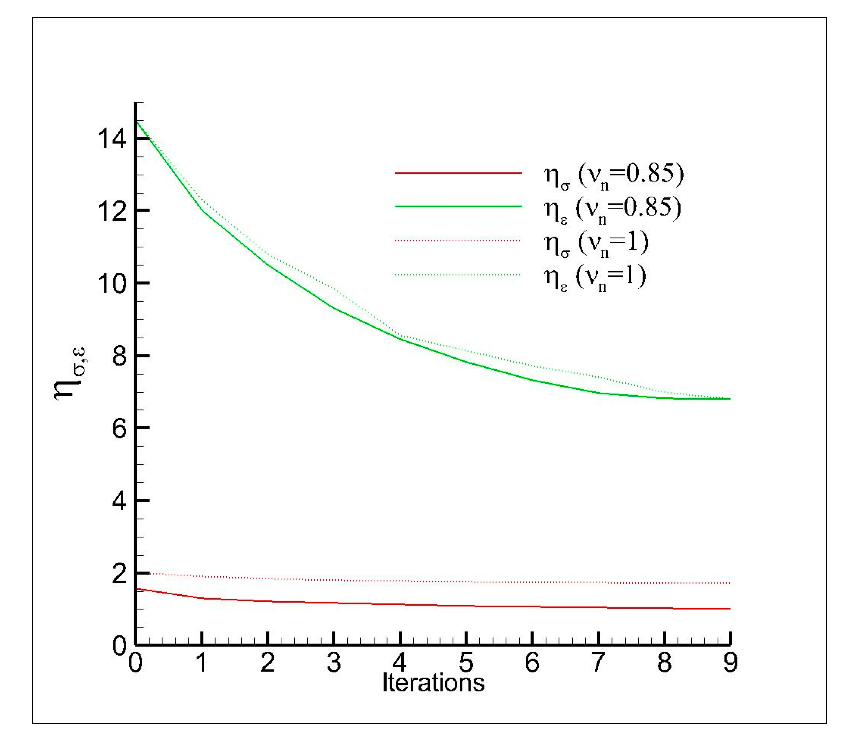
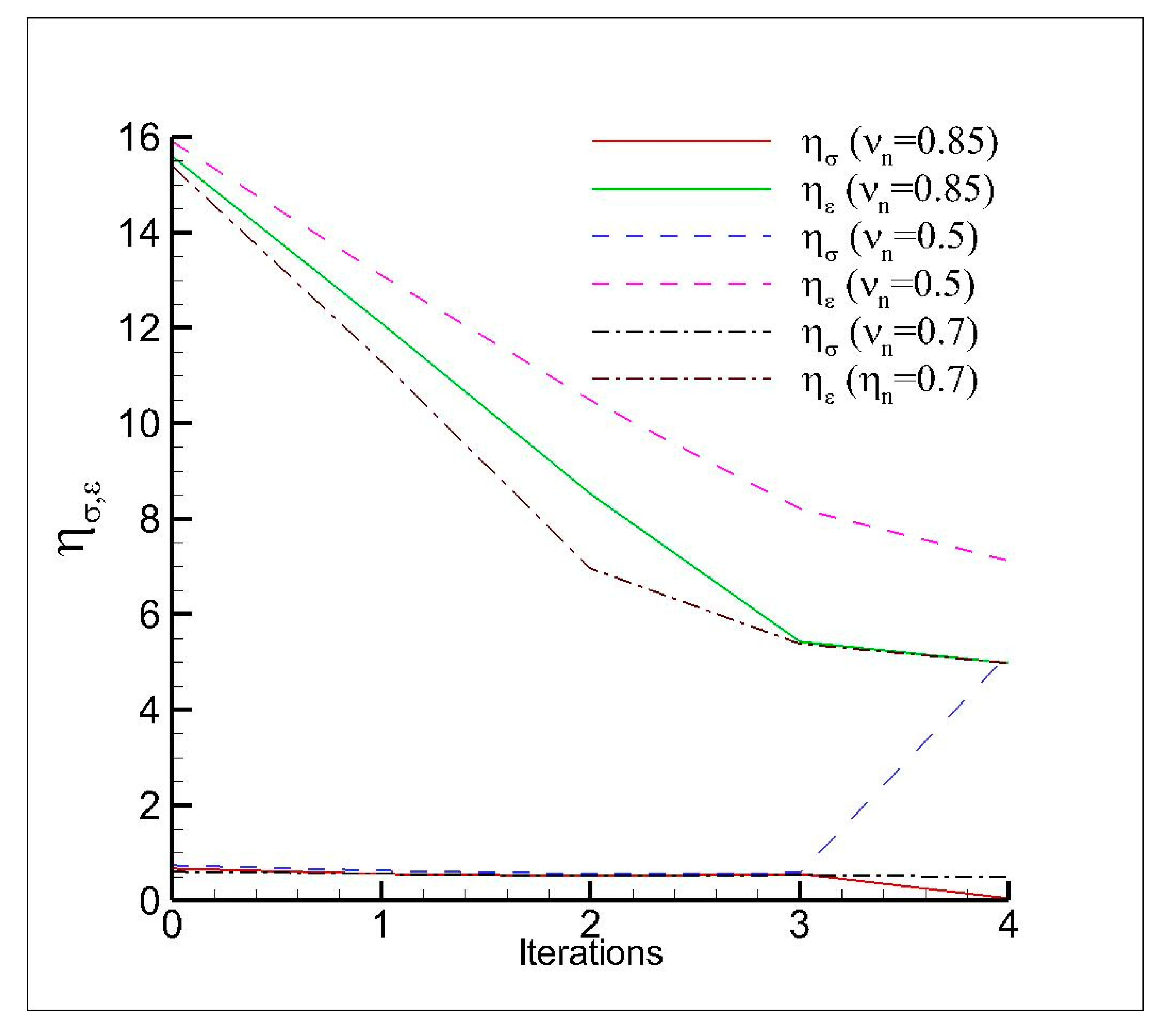
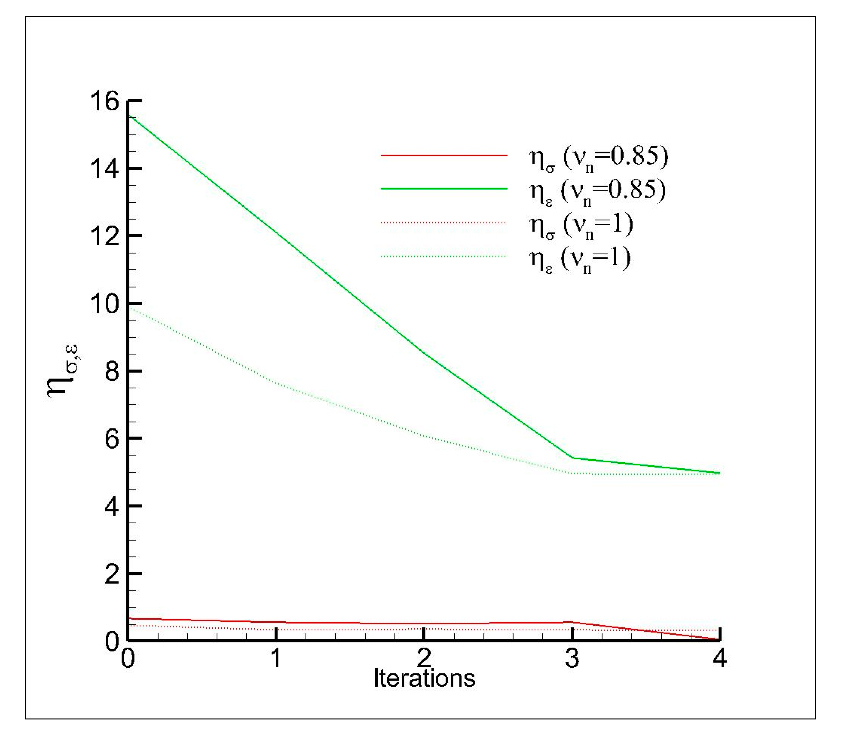
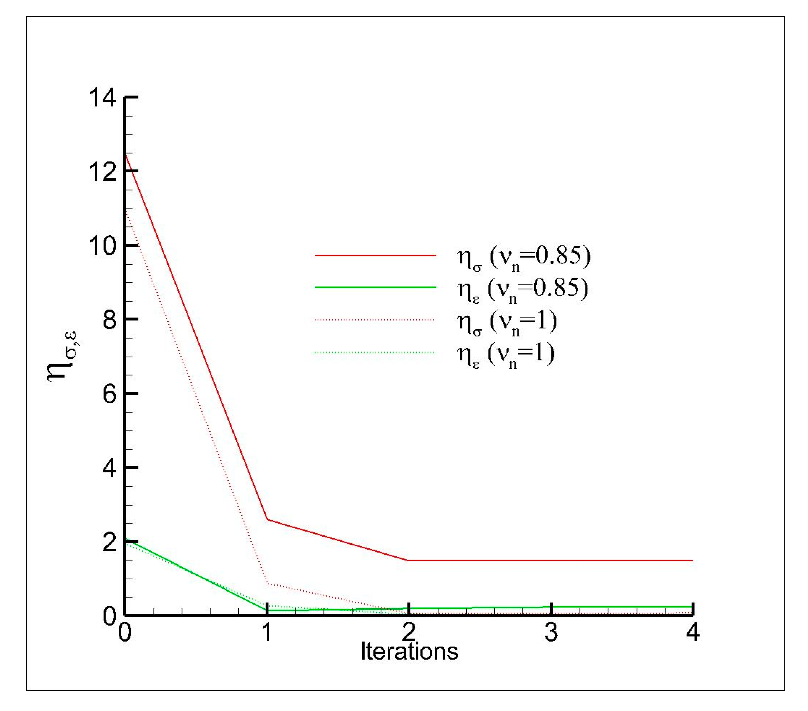
- is the equivalent plastic strain calculated by the Global/Local approach,
- is the equivalent plastic strain calculated by the Reference Model,
- is the Von Mises stress evaluated by the Global/Local approach,
- is the Von Mises stress evaluated by the Reference Model,
- can be equal to 2 (Euclidean norm) or ∞ (infinite norm).
4.2. Numerical Discretization
- 20000 (Reference Model)
- 3700 (Global Model)
- 16300 (Local Model)
4.3. Material Properties
5. Results and Discussion
5.1. Two–Dimensional Global/Local Analyses
Trade-Off Analysis with Non-Conformal Meshes
5.2. Three–Dimensional Global/Local Analyses
6. Conclusions and Future Activities
Author Contributions
Funding
Acknowledgments
Conflicts of Interest
Nomenclature
| temperature | |
| time | |
| Cauchy Stresses tensor | |
| body force per unit volume | |
| elastic strain tensor | |
| plastic strain tensor | |
| plastic work | |
| back stress tensor | |
| E | Young Modulus |
| K | plastic modulus |
| deviatoric stress tensor | |
| plastic multiplier | |
| interface curve/surface | |
| vector of nodal forces on surface (local model) | |
| vector of nodal forces on surface (global model) | |
| displacement on | |
| Euclidean norm of the vector | |
| convective coefficients for the combustion gases | |
| convective coefficients for the coolant | |
| combustion gases bulk temperature | |
| coolant bulk temperature | |
| non–dimensional parameter to measure strain accuracy | |
| non–dimensional parameter to measure stress accuracy |
References
- Salvatore, V.; Battista, F.; Votta, R.; Di Clemente, M.; Ferraiuolo, M.; Roncioni, P.; Ricci, D.; Natale, P.; Panelli, M.; Cardillo, D.; et al. Design and Development of a LOX/LCH4 Technology Demonstrator. In Proceedings of the 48th AIAA/ASME/SAE/ASEE Joint Propulsion Conference & Exhibi, Atlanta, GA, USA, 30 July–1 August 2012. [Google Scholar]
- Haeseler, D.; Bombelli, V.; Vuillermoz, P.; Lo, R.; Marée, T.; Caramelli, F. Green Propellant Propulsion Concepts for Space Transportation and Technology Development Needs. In Proceedings of the 2nd International Conference on Green propellants for Space, Propulsion, Sardinia, Italy, 7–8 June 2004. [Google Scholar]
- Haeseler, D.; Mäding, C.; Götz, A.; Roubinski, V.; Khrissanfov, S.; Berejnoy, V.; Bureau, C.D. Recent Developments for Future Launch Vehicle LOX/HC Rocket Engines. In Proceedings of the 6th International Symposium Propulsion for Space Transportation of the XXIst Century, Versailles, France, 13–17 May 2002. [Google Scholar]
- Collins, J.; Hurlbert, E.; Romig, K.; Melcher, J.; Hobson, A.; Eaton, P. Sea-Level Flight Demonstration &Altitude Characterization of a LO2/LCH4 Based Ascent Propulsion Lander. In Proceedings of the 45th AIAA/ASME/SAE/ASEE Joint Propulsion Conference & Exhibit, Denver, CO, USA, 2–5 August 2009; p. 4948. [Google Scholar]
- Battista, F.; Di Clemente, M.; Ferraiuolo, M.; Votta, R.; Ricci, D.; Panelli, M.; Roncioni, P.; Cardillo, D.; Natale, P.; Salvatore, V. Development of a LOX/LCH4 Technology Demonstrator Based on Regenerative Cooling throughout Validation of Critical Design Aspects with Breadboards in the Framework of the Hyprob Program. In Proceedings of the 63rd International Astronautical Congress, Naples, Italy, 1–5 October 2012. [Google Scholar]
- Brown, C.D. Conceptual Investigations for a Methane-Fueled Expander Rocket Engine. In Proceedings of the 40th AIAA/ASME/SAE/ASEE Joint Propulsion Conference and Exhibit, Fort Lauderdale, FL, USA, 11–14 July 2004; p. 4210. [Google Scholar]
- Ferraiuolo, M.; Riccio, A. Study of the Effects of Materials Selection for the Closeout Structure on the Service Life of a Liquid Rocket Engine Thrust Chamber. J. Mater. Eng. Perform. 2019, 28, 3186–3195. [Google Scholar] [CrossRef]
- Ferraiuolo, M.; Russo, V.; Vafai, K. A comparative study of refined and simplified thermo-viscoplastic modeling of a thrust chamber with regenerative cooling. Int. Commun. Heat Mass Transf. 2016, 78, 155–162. [Google Scholar] [CrossRef]
- Arya, V.K.; Arnold, S.M. Viscoplastic Analysis of an Experimental Cylindrical Thrust Chamber Liner. AIAA J. 1992, 30, 781–789. [Google Scholar] [CrossRef] [Green Version]
- Riccius, J.R.; Hilsenbeck, M.R.; Haidn, O.J. Optimization of geometric parameters of cryogenic liquid rocket combustion chambers. In Proceedings of the 37th AIAA/ASME/SAE/ASEE JPC, Salt Lake City, UT, USA, 8–11 July 2001. [Google Scholar]
- Maire, J.F.; Chaboche, J.L. A new formulation of continuum damage mechanics (CDM) for composite materials. Aerosp. Sci. Technol. 1997, 1, 247–257. [Google Scholar] [CrossRef]
- Citarella, R.; Cricrì, G.; Lepore, M.; Perrella, M. Thermo-Mechanical Crack Propagation in Aircraft Engine Vane by Coupled FEM-DBEM Approach. Adv. Eng. Softw. 2014, 67, 57–69. [Google Scholar] [CrossRef]
- Guinard, S.; Bouclier, R.; Toniolli, M.; Passieux, J.C. Multiscale analysis of complex aeronautical structures using robust non-intrusive coupling. Adv. Model. Simul. Eng. Sci. 2018, 5, 1–27. [Google Scholar] [CrossRef] [Green Version]
- Ferraiuolo, M.; Palumbo, C.; Sellitto, A.; Riccio, A. Investigating the Thermo-Mechanical Behavior of a Ceramic Matrix Composite Wing Leading Edge by Sub-Modeling Based Numerical Analyses. Computation 2020, 8, 22. [Google Scholar] [CrossRef] [Green Version]
- Gendre, L.; Allix, O.; Gosselet, P.; Comte, F. Non-Intrusive and Exact Global/Local Techniques for Structural Problems with Local Plasticity; Computational Mechanics; Springer: New York, NY, USA, 2009; Volume 44, pp. 233–245. hal-00437023. [Google Scholar] [CrossRef]
- Citarella, R.; Cricrì, G.; Lepore, M.; Perrella, M. Assessment of Crack Growth from a Cold Worked Hole by Coupled FEM-DBEM Approach. In Key Engineering Materials; Trans Tech Publications: Bach, Switzerland, 2014; Volume 577–578, pp. 669–672. [Google Scholar]
- Citarella, R.; Cricrì, G.; Armentani, E. Multiple crack propagation with Dual Boundary Element Method in stiffened and reinforced full scale aeronautic panels. In Key Engineering Materials; Trans Tech Publications: Bach, Switzerland, 2013; pp. 129–155. [Google Scholar]
- Citarella, R. Non Linear MSD crack growth by DBEM for a riveted aeronautic reinforcement. Adv. Eng. Softw. 2009, 40, 253–259. [Google Scholar] [CrossRef]
- Passieux, J.C.; Réthoré, J.; Gravouil, A.; Baietto, M.C. Local/global non-intrusive crack propagation simulation using a multigrid X-FEM solver. Comput. Mech. 2013, 52, 1381–1393. [Google Scholar] [CrossRef] [Green Version]
- Gosselet, P.; Blanchard, M.; Allix, O.; Guguin, G. Non-invasive global–local coupling as a Schwarz domain decomposition method: Acceleration and generalization. Adv. Model. Simul. Eng. Sci. 2018, 4, 5. [Google Scholar] [CrossRef] [Green Version]
- Ozisik, N. Heat Conduction; Wiley: New York, NY, USA, 1980. [Google Scholar]
- Ferraiuolo, M.; Ricci, D.; Battista, F.; Roncioni, P.; Salvatore, V. Thermo-structural and thermo-fluid dynamics analyses supporting the design of the cooling system of a methane liquid rocket engine. In ASME International Mechanical Engineering Congress and Exposition; American Society of Mechanical Engineers: Montreal, QC, Canada, 2014. [Google Scholar] [CrossRef]
- Henson, G. Chapter 7: Materials for Launch Vehicle Structures; American Institute of Aeronautics and Astronautics: Westlake, OH, USA, 2017; p. 0001809. [Google Scholar]
- Riccius, J.R.; Haidn, O.J.; Zametaev, E.B. Influence of time dependent effects on the estimated life time of liquid rocket combustion chamber walls. In Proceedings of the 40th AIAA/ASME/SAE/ASEE Joint Propulsion Conference, Fort Lauderdale, FL, USA, 11–14 July 2004; p. 3670. [Google Scholar]
- Thiede, R.G.; Riccius, J.R.; Reese, S. Life Prediction of Rocket Combustion-Chamber-Type Thermomechanical Fatigue Panels. J. Propuls. Power 2017, 33, 1529–1542. [Google Scholar] [CrossRef]
- Quentmeyer, R.J. Experimental fatigue life investigation of cylindrical thrust chambers. In Proceedings of the 13th Propulsion Conference, Orlando, FL, USA, 11–13 July 1977. [Google Scholar]
- Armstrong, W.H. Final Kept. NASA Lewis Research Center, NASA-CR-159552, Contract NASA-21361, Structural Analysis of Cylindrical Thrust Chamber; NASA: Hampton, VI, USA, 1979; Volume I.
- Arya, V.K.; Halford, G.R. Finite element analysis of structural engineering problems using a viscoplastic model incorporating two back stresses. In Proceedings of the International Seminar on Inelastic Analysis, Fracture and Life Prediction, Paris, France, 24–25 August 1993. NASA TM-106046. [Google Scholar]
- Freed, A.D. Structure of a viscoplastic theory, Constitutive Equations and Life Prediction Models for High Temperature Applications Symposium; NASA TM-100749, Sponsored by American Society of Mechanical Engineers; NASA Lewis Research Center: Berkeley, CA, USA, 1988.
- Zhang, Y.; Zhang, Q.; Qin, X.; Sun, Y. A Consistent Relationship between the Stress and Plastic Strain Components and Its Application in Deep Drawing Process. Math. Probl. Eng. 2017, 2017, 4278082. [Google Scholar] [CrossRef]
- Simo, J.C.; Hughes, T.J.R. Computational Inelasticity; Springer: New York, NY, USA, 2006; ISBN 978-0-387-22763-4. [Google Scholar]
- Watson, D.F.; Philip, G.M. Triangle based interpolation. Math. Geol. 1984, 16, 779–795. [Google Scholar] [CrossRef]
- Hetnarski, R.; Eslami, M. Thermal Stresses—Advanced Theory and Application; Springer: Dordrecht, The Netherlands, 2009; ISBN 978-1-4020-9246-6. [Google Scholar]


| a (mm) | b (mm) | s (mm) | t1 (mm) | t2 (mm) |
|---|---|---|---|---|
| 2 | 0.62 | 0.9 | 0.5 | 1.5 |
| 5600 | 280.000 |
| 3600 | 370 |
| Temperature (K) | Density (kg/m3) | Thermal Conductivity (W/mK) | Specific Heat (J/kgK) | Thermal Expansion Coefficient (1/K) |
|---|---|---|---|---|
| 300 | 8933 | 320 | 390 | 15.7 × 10⁻⁶ |
| 600 | 8933 | 290 | 390 | 17.9 × 10⁻⁶ |
| 900 | 8933 | 255 | 400 | 18.7 × 10⁻⁶ |
| Temperature (K) | E (Gpa) | Poisson’s Ratio | Yield Stress (MPa) | Ultimate Stress (MPa) |
|---|---|---|---|---|
| 300 | 130 | 0.3 | 4339 | 4779 |
| 500 | 106 | 0.3 | 3833 | 4029 |
| 700 | 87 | 0.3 | 313 | 3294 |
| 900 | 44 | 0.3 | 1563 | 1754 |
| Temperature (K) | Density (kg/m3) | Thermal Conductivity (W/mK) | Specific Heat (J/kgK) | Thermal Expansion Coefficient (1/K) |
|---|---|---|---|---|
| 300 | 8913 | 390 | 385 | 17.2 × 10⁻⁶ |
| Temperature (K) | E (Gpa) | Poisson’s Ratio | Yield Stress (MPa) | Ultimate Stress (MPa) |
|---|---|---|---|---|
| 28 | 118 | 0.34 | 68 | 413 |
| 294 | 114 | 0.34 | 60 | 208 |
| 533 | 65 | 0.34 | 50 | 145 |
| 755 | 40 | 0.34 | 38 | 80 |
| Temperature (K) | Density (kg/m3) | Thermal Conductivity (W/mK) | Specific Heat (J/kgK) | Thermal Expansion Coefficient (1/K) |
|---|---|---|---|---|
| 300 | 8913 | 90 | 444 | 12.2 × 10⁻⁶ |
| Temperature (K) | E (Gpa) | Yield Stress (MPa) | Ultimate Stress (MPa) | Poisson’s Ratio |
|---|---|---|---|---|
| 28 | 193 | 344 | 551 | 0.3 |
| Local Model 4 | Local Model 5 | |
|---|---|---|
| (%)–iteration 0 | 10 | 8 |
| (%)–iteration 1 | 5 | 4.8 |
| Local Models | Nodes: Global Coarse Model (Conformal Mesh) | Nodes: Global Coarse Model (Non–Conformal Mesh) | Nodes: Local Model | CPU Time (Conformal Mesh) (s) | CPU Time (Non–Conformal Mesh) (s) | CPU Time (Reference Model) (s) |
|---|---|---|---|---|---|---|
| y = 0.5 | 4800 | 4700 | 10,000 | 50 | 38 | 150 |
| y = 0.9 | 4600 | 3864 | 15,000 | 26 | 22 | 150 |
| y = 1.2 | 4600 | 3864 | 17,500 | 50 | 48 | 150 |
| y = 1.5 | 4600 | 3864 | 18,200 | 52 | 50 | 150 |
| y = 1.8 | 4600 | 3864 | 18,800 | 53 | 50 | 150 |
Publisher’s Note: MDPI stays neutral with regard to jurisdictional claims in published maps and institutional affiliations. |
© 2020 by the authors. Licensee MDPI, Basel, Switzerland. This article is an open access article distributed under the terms and conditions of the Creative Commons Attribution (CC BY) license (http://creativecommons.org/licenses/by/4.0/).
Share and Cite
Ferraiuolo, M.; Leo, M.; Citarella, R. On the Adoption of Global/Local Approaches for the Thermomechanical Analysis and Design of Liquid Rocket Engines. Appl. Sci. 2020, 10, 7664. https://doi.org/10.3390/app10217664
Ferraiuolo M, Leo M, Citarella R. On the Adoption of Global/Local Approaches for the Thermomechanical Analysis and Design of Liquid Rocket Engines. Applied Sciences. 2020; 10(21):7664. https://doi.org/10.3390/app10217664
Chicago/Turabian StyleFerraiuolo, Michele, Michele Leo, and Roberto Citarella. 2020. "On the Adoption of Global/Local Approaches for the Thermomechanical Analysis and Design of Liquid Rocket Engines" Applied Sciences 10, no. 21: 7664. https://doi.org/10.3390/app10217664