Scaling Law, Confined and Surface Modes in Photonic Fibonacci Stub Structures: Theory and Experiment

Abstract

We investigate both theoretically and experimentally the properties of electromagnetic waves propagation and localization in periodic and quasi-periodic stub structures of Fibonacci type. Each block constituting the Fibonacci sequence (FS) is composed of an horizontal segment and a vertical stub. The origin of the primary and secondary gaps shown in such systems is discussed. The behaviors and scattering properties of the electromagnetic modes are studied in two geometries, when the FS is inserted horizontally between two semi-infinite waveguides or grafted vertically along a guide. Typical properties of the Fibonacci systems such as the fragmentation of the frequency spectrum, the self-similarity following a scaling law are analyzed and discussed. It is found that certain modes inside these two geometries decrease according to a power law rather than an exponential law and the localization of these modes displays the property of self-similarity around the central gap frequency of the periodic structure where the quasi-periodicity is most effective. Also, the eigenmodes of the FS of different generation order are studied depending on the boundary conditions imposed on its extremities. It is shown that both geometries provide complementary information on the localization of the different modes inside the FS. In particular, in addition to bulk modes, some localized modes induced by both extremities of the system exhibit different behaviors depending on which surface they are localized. The theory is carried out using the Green’s function approach through an analysis of the dispersion relation, transmission coefficient and electric field distribution through such finite structures. The theoretical findings are in good agreement with the experimental results performed by measuring in the radio-frequency range the transmission along a waveguide in which the FS is inserted horizontally or grafted vertically.

1. Introduction

After decades of extensive studies focusing on periodic crystals, scientific research interest have also been extended to quasi-periodic crystals. These structures were discovered by Dan Shechtman [1] in metallic Al-Mn alloys in 1984, for which he earned the Nobel Prize in Chemistry 2011. The samples of such alloys exhibit a high degree of symmetry including the fivefold and icosahedral symmetries, which is prohibited by the rules of crystallography [1,2,3] and possess a long-range orientational order instead of a translational symmetry typical of a conventional crystal. The fascinating features of the quasiperiodic structures are that they have multiple frequency band gap regions similar to the band gaps of periodic crystals, due to the presence of more than one form of periodicity across these structures. Moreover, they exhibit transmission resonances and critical localized states [4]. The peculiar properties of quasi-crystals are strongly useful for the conception of potential applications in different domains [5,6], especially optical communications technology such as optical filter [7,8,9], optical fibers [10,11], microcavities and lasers [12,13,14,15,16], lenses [17], sensors [18,19] etc.

Studies of lower dimensional systems such as one dimensional (1D) layered media, waveguides and aperiodic linear chains are performed as in their 2D and 3D analogues with different applications [4,5]. Indeed, it was shown that 1D models can be considered as a first approximation to the study of higher dimensional quasiperiodic systems [4]. Quasiperiodic structures could be structured following different types of sequences such as Fibonacci [20], Thue-Morse [21,22], Rudin-Shapiro [23], Double period [24,25] and Cantor [26,27,28]. The most well known of these systems is the Fibonacci structures [29], which have been widely studied for several types of excitations such as electrons [30,31], phonons [32,33,34,35], photons [36,37], magnons [38] and plasmons [39,40,41]. Merlin et al. [30] produced first Fibonacci structures based on GaAs-AlAs semiconductor superlattices. Since this work, several works have been devoted to observe the exotic phenomena of Fibonacci systems [42,43] and different interesting properties have been found [44] essentially by theoretical studies using simple 1D models. Kohmoto et al. [31] investigated the electronic features of a 1D quasi-periodic structure organized along a Fibonacci sequence such as the self-similarity and other critical properties of the wave functions. The first calculations of the phonon dispersion relations in a Fibonacci superlattice was developed by Tamura et al. [32] and a number of transmission dips associated with Bragg-like reflections of phonons has been found. In addition, a theoretical study for the propagation and localization of acoustic waves in a Fibonacci waveguide structure made of slender loop tubes connected together by slender tubes has been investigated by Aynaou et al. [33] and experimentally checked by King and Cox [45]. Kohmoto et al. [36] have found that the transmission coefficient is multi-fractal and the resonance modes exhibit scaling behavior. The first experiment on photonic quasi-crystal based on the Fibonacci sequence has been reported by Hattori et al. [37]. It was shown that the phase spectrum exhibits clearly the self-similar structure of the dispersion curves typical of Fibonacci lattices. The research in Refs. [36,37] have generated a large amount of theoretical and experimental research activity in the field of 1D, 2D and 3D photonic quasi-crystals with numerous device and engineering applications [5,6,46]. It was demonstrated that these systems exhibit fascinating properties like the occurrence of multiple forbidden frequency regions, self-similar spectrum and critical behavior of resonance modes, which can present an interesting alternative to ordinary photonic crystals for the design of new photonic devices [47,48,49,50,51,52,53,54,55,56,57,58,59].

In addition to the multi-layer structures, few works have been devoted to quasi-periodic coaxial photonic crystals by some of us [60,61,62]. In Ref. [60] Aynaou et al. studied the localization and propagation of electromagnetic waves in a Fibonacci coaxial photonic circuits made of two blocks in which each block is composed by a loop and segment arranged following a FS. They have found that the symmetrical loop structure is equivalent to simple alternating layers. However, the asymmetrical loops play the role of resonators giving rise to transmission zeros (like in Mach-Zehnder interferometer [63]) and hence new gaps which does not exist in the case of layered media. El Boudouti et al. [61] have examined the properties of Fibonacci 1D serial loop structures where each block is made of a segment or a loop. Particular properties have been deduced when the FS was inserted horizontally between two waveguides or attached vertically along a guide, such as self-similarity, scaling behavior and critical localized modes. Furthermore El Hassouani et al. [62] have extensively studied the behavior of the surface modes in Fibonacci superlattices made from a periodic repetition of a given Fibonacci generation.

It is worth mentioning that a number of interesting physical properties related to the electronic transport, charge density distribution and energy spectra in periodic and Fibonacci stub structures have been performed theoretically by Jin et al. [64] and Nomata and Horie [65]. Also, Chattopadhyay et al. [66] have developed a method showing the single-electron transport through quantum stub waveguides arranged in a Fibonacci quasi-periodic pattern. The similarity between scattering properties (equation of motion and boundary conditions) of electrons and photons, points out that this type of features can also appear for photons [67]. Furthermore, because of their noninteracting nature, electromagnetic waves represent an interesting tool for studying the localization phenomena [37,47] in comparison with electrons. Therefore, photonic circuits based coaxial cables represent an excellent platform to observe several properties of Fibonacci stubbed structures. Indeed, these systems are more appealing for this goal than their optical counterparts since they only require simple equipments. In addition, the propagation in these waveguides is monomode (see below) and one can obtain experimental results with a good precision as well as theoretical results using a simple 1D model with a very good agreement between both results [67].

In this paper, we give a theoretical and experimental study of the localization and propagation of electromagnetic waves in Fibonacci stub structures. Such structures have been studied only for periodic structures with or without defects [68,69]. However, to our knowledge, no similar study has been carried out for photonic Fibonacci structures. In this work, a theoretical and an experimental evidence of the features of the transmission modes through a Fibonacci stubbed circuit structure inserted either between two semi-infinite waveguides or grafted vertically along a guide are investigated. The geometry of the FS proposed here is original and simple in comparison with the symmetrical loop geometries studied before [60,61,62] as the stubs may present transmission zeros which do not exist in loop structures, also the boundary conditions on the stub extremities can be changed easily which is not the case for loop systems. Furthermore, the study of the FS in the two geometries (horizontal and vertical) enables us to deduce typical properties of these systems such as: (i) the fragmentation of the frequency spectrum into small bands and primary and secondary gaps, (ii) the self-similarity of the modes in the transmission spectra as well as in the electric field distribution around a central frequency where the quasi-periodicity is more effective, (iii) the analysis of the behavior of the eigenmodes of the FS with different boundary conditions imposed on its both extremities. These modes are obtained by means of a theorem developed by some of us earlier [70,71] in which the eigenmodes of a finite system can be deduced directly from the maxima or minima of the transmission coefficient when this system is grafted vertically along a waveguide. Among these modes, there exist different surface modes which depend on the surface termination of the FS. (iv) The study of the transition between periodic and quasi-periodic structures in the transmission spectra, when the former is perturbed progressively towards the latter and vice-versa.

As mentioned above, both geometries (horizontal and vertical) provide complementary informations on the localization and propagation of different modes in the FS. However the vertical structure is rich of information as it enables to extract also the confined and surface modes of the finite photonic Fibonacci crystal with different boundary conditions on its extremities. The latter boundary modes are found quantitatively equivalent to those of the Harper model [72] in a Fibonacci photonic quasicrystal [73], showing their topological origin [74]. The experiments are carried out using coaxial cables in the radio-frequency region and the theoretical approach is based on the Green’s function formalism which enables us to deduce the dispersion relations, transmission coefficients and densities of states (DOS).

This paper is organized as follows: Section 2 is devoted to the theoretical model based on the Green’s function approach to derive the expressions of transmission coefficients, densities of states and dispersion relations, whereas the experimental procedure is described in Section 3. The numerical and experimental results are provided in Section 4, when the Fibonacci stub structure is inserted horizontally between two semi-infinite guides or connected vertically along a guide. Finally, a brief summary of the main results of this paper is presented in the conclusion.

2. Theoretical Approach: Green’s Function

We consider a 1D quasi-periodic structure composed of two blocks A and B stacked following the Fibonacci sequence [29]: $S_{k+1}=S_k{S}_{k-1}$ with the initial conditions $S_1=A$ and $S_2=AB$, where $S_k$ is the kth generation of the Fibonacci sequence. For exemple $S_3=ABA$, $S_4=ABAAB$, $S_5=ABAABABA$,.... For the Fibonnaci structures considered here (Figure 1), the block A is formed of identical horizontal and vertical coaxial cables of length $d_2=d_1$ (Figure 1a), while the Block B is similar to the block A but with different length of its vertical cable, namely $d_3=d_2/2$ (Figure 1b). All coaxial cables are characterized by the same impedance Z.

The localization and the propagation of electromagnetic waves in the Fibonacci structures depicted in Figure 1f,g, are performed within the framework of the interface response theory of continuous media [75]. This theory enables to calculate the Green’s function of any heterogenous system containing a large number of interfaces separating different homogenous media. In what follows, the fundamental equations and the basic concepts of this theory [75] are presented. We consider an heterogenous system composed of N different homogeneous sub-systems defined in their domains $D_i$ ($D=\bigcup D_i$ being the whole space of the system). Each subsystem “i” is connected in general to j$(1\le j\le J)$ other pieces through sub-interface domains $M_{ij}$ ($M_i=\bigcup M_{ij}$ being the interface space of the sub-system “i”). All these interface spaces $M_i$ constitutes what is called the interface space M of the heterogenous material. In this theory, the elements of the Green’s function $g\left(DD\right)$ of a composite material is given by [75]

$$\begin{array}{ccc}\hfill g\left(DD\right)& =& G\left(DD\right)-G\left(DM\right)G^{-1}\left(MM\right)G\left(MD\right)\hfill \\ \hfill & & +G\left(DM\right)G^{-1}\left(MM\right)g\left(MM\right)G^{-1}\left(MM\right)G\left(MD\right),\hfill \end{array}$$

(1)

where $G\left(DD\right)$ is the reference Green’s function constituted from the superposition of the truncated bulk Green’s functions of each piece defined in its space domain $D_i$. $g\left(MM\right)$ corresponds to the Green’s function of the composite system in the whole interface space M. The inverse of $g\left(MM\right)$ enables to calculate the dispersion relations of the composite system using the following expression [75]

$$det\left[g^{-1}\left(MM\right)\right]=0.$$

(2)

Also, using this theory, Equation (1) enables to calculate the eigenvectors $u\left(D\right)$ of the composite material from the relation [75]

$$\begin{array}{ccc}\hfill u\left(D\right)& =& U\left(D\right)-U\left(M\right)G^{-1}\left(MM\right)G\left(MD\right)+\hfill \\ \hfill & & U\left(M\right)G^{-1}\left(MM\right)g\left(MM\right)G^{-1}\left(MM\right)G\left(MD\right),\hfill \end{array}$$

(3)

where $U\left(D\right)$, $U\left(M\right)$ and $u\left(D\right)$ are row vectors. In particular, if $U\left(D\right)$ represents a bulk wave launched in one homogeneous piece of the whole system [67], then Equation (3) enables to calculate the transmission and reflection coefficients through the system.

The calculation of the Green’s function of a FS in the whole interface space M, requires the knowledge of the surface elements of its elementary constituents, namely, the Green’s function of the block A (Figure 1a) and of the block B (Figure 1b). The explicit expressions of the 2 × 2 matrices of these two blocks are given by Equations (A6) and (A7) in the Appendix A. Also, the method for deriving the inverse surface Green’s function matrix of the whole FS (Figure 1c–e) is described in the Appendix A for the 4th generation for example. $g_{FS}^{-1}\left(M_e{M}_e\right)$ can be written as

$${\left[g_{FS}\left(M_e{M}_e\right)\right]}^{-1}=\left(\begin{array}{cc}a& b\\ b& c\end{array}\right),$$

(4)

where $M_e=\{0,L\}$ is the space of interfaces at both free extremities of a given FS and L is the total length of the structure. a, b and c are real quantities, functions of the different parameters of the constituent’s elements. The derivation of these parameters is described in Equations (A6) and (A7) of the Appendix A.

Let us consider the finite FS structure delimited by two homogeneous semi-infinite waveguides labeled s characterized by their inverse surface Green’s function at the surface $x=0$ or $x=L$ (see Equation (A5) in the Appendix A)

$$g_s{(0,0)}^{-1}=g_s{(L,L)}^{-1}=-F_s,$$

(5)

where $F_s=-j\omega /Z_s$, $Z_s$ is the impedance of semi-infinite waveguide and $\omega$ is the angular frequency. Then the inverse Green’s function of the whole horizontal composite system (Figure 1f) can be obtained from a superposition of the matrix given in Equation (4) surrounded by two semi-infinite waveguides on both sides (Equation (5)) such as

$${\left[g_h\left(M_e{M}_e\right)\right]}^{-1}=\left(\begin{array}{cc}a-F_s& b\\ b& c-F_s\end{array}\right).$$

(6)

Similarly, the inverse Green’s function of the whole vertical system (Figure 1g) can be obtained from a superposition of the matrix given in Equation (4) surrounded by two semi-infinite waveguides on one side (Equation (5)) such as

$${\left[g_v\left(M_e{M}_e\right)\right]}^{-1}=\left(\begin{array}{cc}a-2F_s& b\\ b& c\end{array}\right).$$

(7)

Here h and v stand for horizontal and vertical insertion of the finite FS. As a preliminary remark, let us notice from Equations (2) and (7) that one can deduce the expressions giving the eigenmodes of the Fibonacci sequence in two particular cases:

(i)

when the magnetic field vanishes on both sides of the FS structure (i.e., $Z_s\to \infty$ or equivalently $F_s=0$), one obtains:

$$ac-b^2=0.$$

(8)

(ii)

When the electric field vanishes on the side of the structure which will be grafted on the waveguide and the magnetic field vanishes on the free surface (i.e., $Z_s=0$ or $F_s\to \infty$), one obtains:

$$c=0.$$

(9)

Now, the determination of the properties of wave propagation and localization in a Fibonacci system inserted (grafted) horizontally (vertically) between two homogeneous waveguides labeled s (Figure 1f,g), requires the calculation of the transmission coefficient of an incident plane wave launched from the left semi-infinite waveguide and traveling through the system. From the bulk Green’s function (Equation (A1)) and Equations (6) and (7), one can get the transmission functions for the horizontal and vertical structures such as: $t_h=-2F_s{g}_h(0,L)$ and $t_v=-2F_s{g}_v(0,0)$ respectively. Therefore, one obtains

$$t_h=\frac{-2F_{s}b}{ac-b^2-{\left(F_s\right)}^2-(a+c)F_s},$$

(10)

and

$$t_v=\frac{-2F_{s}c}{ac-b^2-2F_{s}c}.$$

(11)

Let us notice that from Equation (11), the eigenmodes of the FS with the boundary conditions of type $E=0$ on one side and $H=0$ on the other side (Equation (9)) are obtained from $t_v=0$ (i.e., c = 0) and the eigenmodes of the FS with the boundary conditions of type $H=0$ on both sides (Equation (8)) are obtained from $t_v=1$ (i.e., $ac-b^2=0$).

3. Experimental Procedure

The experiments were performed using standard coaxial cables with different lengths and identical characteristic impedance $Z_c$, combined with metallic T-shaped connectors. The validity of our results is subject to the requirement that the cross section of the waveguide is negligible compared to their length and to the propagation wavelength. Indeed, it is well established that within such assumption and for frequencies below the cut-off frequency ($f_c$), only transverse electromagnetic modes (TEM) can propagate. The threshold frequency $f_c$ below which the propagation becomes monomode, is given by [76]

$$f_c=190.85/\left({\epsilon }_r(d_{out}+d_{in})\right)\left(GHz\right),$$

(12)

where $d_{out}=3\pm 0.1$ mm is the dielectric diameter (i.e., the interior diameter of the outer conductor), $d_{in}=0.8\pm 0.02$ mm is the diameter of the inner conductor and ${\epsilon }_r$ is the dielectric permittivity (${\epsilon }_r=2.3$) of the polyethylene between the two conductors, which corresponds to a nominal propagation speed of $0.66c$. For $d_{out}=3$ mm and $d_{in}=0.8$ mm, one obtains $f_c=33.11$ GHz which is sufficiently above the domain of frequencies considered in this work.

The characteristic impedance $Z_c$ of the cables is given by [76]

$$Z_c=138log(d_{out}/d_{in})/\sqrt{{\epsilon }_r}.$$

(13)

From the above values of $d_{out}$ and $d_{in}$, one can find the characteristic impedance $Z_c=50\pm 3\mathsf{\Omega }$. The electromagnetic impedance at the free ends of the resonators of lengths $d_2$ (Figure 1a) and $d_3$ (Figure 1b), may be adapted in order to realize the boundary condition $E=0$ (short-circuit) or $H=0$ (open-circuit).

The experimental measurements (including the amplitude and the phase of the transmission coefficients) were measured in the frequency range 0–200 MHz by means of a broadband vector network analyzer (VNA) Agilent PNA-X N5242A. The VNA allows accurate measurements of the four S parameters with an error less than $0.2\%$. The uncertainty on the measurements of the amplitude and phase are around $0.5$ mV and 0.01${}^{\circ }$ respectively.

The attenuation inside the coaxial cables was simulated by introducing a relative dielectric permittivity $\epsilon$ $(\epsilon ={\epsilon }^{\prime }-j{\epsilon }^{″})$ where ${\epsilon }^{\prime }$ and ${\epsilon }^{″}$ are the real and imaginary parts of the dielectric permittivity respectively. The attenuation coefficient ${\alpha }^{″}$ can be expressed as ${\alpha }^{″}={\epsilon }^{″}\omega /c$. From the data supplied by the manufacturer of the coaxial cables in the frequency range of 0 to 200 MHz, one can deduce a fitted expression of ${\alpha }^{″}$ such as $ln\left({\alpha }^{″}\right)=\gamma +\delta ln\left(\omega \right)$, where $\gamma$ and $\delta$ are two constants. This fitting procedure enables to deduce a useful expression for ${\epsilon }^{″}$ versus the frequency, namely ${\epsilon }^{″}={\left(\frac{f}{f_0}\right)}^{-0.5}$ where the frequency f is expressed in Hz and $f_0=9200$ Hz. Further details and a photograph of the experimental setup can be found elsewhere [77,78].

4. Numerical and Experimental Results

Before developing the numerical and experimental results, we shall give a description of the different geometrical structures considered in this work. As mentioned above the periodic and Fibonacci structures considered here are constituted from two blocks A and B. The block A is made of an horizontal waveguide and a vertical stub of the same length (i.e., $d_1=d_2=1$ m) (Figure 1a). The shape of the block B is made of the same horizontal segment as for the block A (i.e., $d_1=1$ m), whereas the vertical stub is characterized by a different length $d_3=d_2/2=0.5$ m (Figure 1b). Therefore, one obtains the Fibonacci sequences $S_3$ (ABA), $S_4$ (ABAAB) and $S_5$ (ABAABABA)... sketched in Figure 1c–e respectively. For the sake of simplicity, the horizontal segments separating the stubs are chosen similar in such a way that only the stubs follow the Fibonacci rule. However, the theoretical results developed here can be applied also to any lengths of the waveguides constituting the blocks A and B. The particular case of periodic structures can be either obtained from only A blocks or only B blocks. All the waveguides are made of the same standard coaxial cables. The boundary conditions at the ends of the stubs are chosen such that $E=0$ (short-circuited).

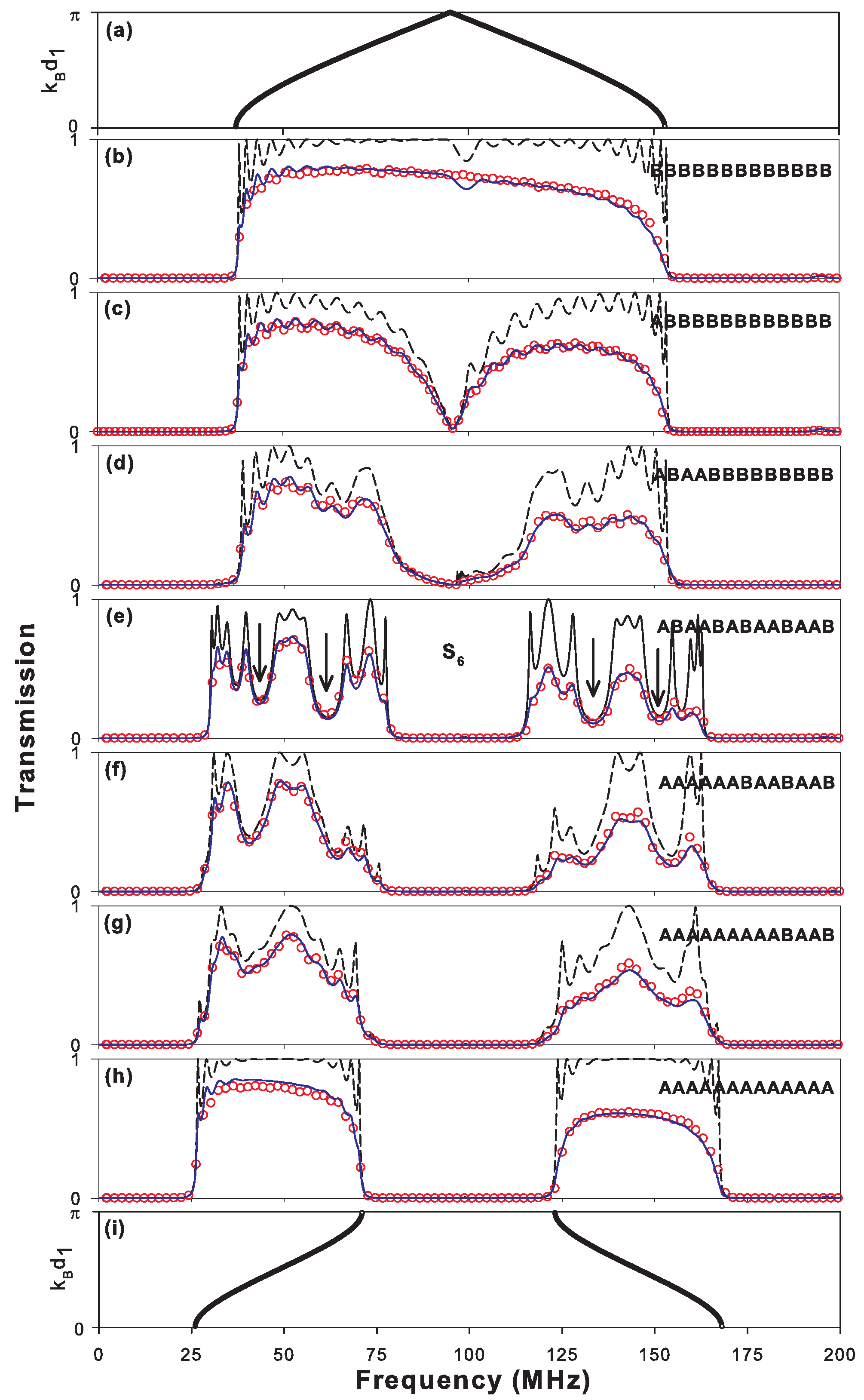
4.1. From Periodic to Fibonacci Sequence and Vice Versa

Before giving the transmission spectra of a given FS composed of A and B blocks, it will be interesting to understand first the dispersion curves of the periodic structures made of only A blocks or only B blocks. The dispersion relation of an infinite periodic comb-like structure constituted by a segment of length $d_1$ and a stub of length $d_m$ (m = 2 or 3) is given by [67]

$$cos\left(k_B{d}_1\right)=cos(\omega d_1\sqrt{\epsilon }/c)+0.5cos(\omega d_m\sqrt{\epsilon }/c)sin(\omega d_1\sqrt{\epsilon }/c)/sin(\omega d_m\sqrt{\epsilon }/c),$$

(14)

where $k_B$ is the Bloch wave-vector.

In the particular case of a periodic structure composed of B blocks (i.e., $d_m=d_3=d_1/2=0.5$ m), then Equation (14) becomes simply $cos\left(k_B{d}_1\right)=3cos(\omega d_1\sqrt{\epsilon }/c)$/2+1/2. Therefore, the band edges are given by $\omega d_1\sqrt{\epsilon }/c=arccos(1/3)$ at the center of the Brillouin zone (BZ) and $\omega d_1\sqrt{\epsilon }/c=\pi$ [mod. $2\pi$] at the limit of the BZ. This result shows that the allowed bands close at the limit of the BZ, whereas the limits of the bands at the center of the BZ are given by $f=38$ MHz and $f=140$ MHz. In addition, the band gaps are periodic every $\omega d_1\sqrt{\epsilon }/c=2\pi$ (i.e., $f=196$ MHz). These results are in accordance with the dispersion curves sketched in Figure 2a inside the first BZ. The transmission spectra through a finite periodic structure composed of 13 B blocks is plotted in Figure 2b. A wide allowed band in the frequency region [38–140] MHz and two gaps at the edges of this band can clearly be observed. The solid (dashed) curves represent the theoretical results with (without) taking into account the dissipation, whereas open circles correspond to the experimental data. Despite the small number of B blocks, the allowed (forbidden) transmission spectra coincide perfectly with the bands (gaps) of the infinite system (Figure 2a). The theoretical results with dissipation (solid curves) are in good agreement with experimental results (open circles). Let us notice that the attenuation inside the cables induces a decay in the transmission amplitude, especially at high frequencies.

Similarly, in the case of a periodic structure composed of A blocks (i.e., $d_m=d_2=d_1=1$ m), then Equation (14) becomes simply $cos\left(k_B{d}_1\right)=3cos(\omega d_1\sqrt{\epsilon }/c)$/2. The band-gap edges are given by $cos\left(k_B{d}_1\right)=\pm 1$ or equivalently $cos(\omega d_1\sqrt{\epsilon }/c)=\pm 2/3$. Therefore, the band edges are given by $\omega d_1\sqrt{\epsilon }/c=arccos(\pm 2/3)$ [mod. $2\pi$]. The first four band limits fall at $f=26$ MHz, $f=72$ MHz, $f=124$ MHz and $f=170$ MHz, in accordance with the dispersion curves sketched in Figure 2i inside the first Brillouin zone. The transmission spectra through a finite periodic structure composed of 13 A blocks is plotted in Figure 2h. Here also, the allowed (forbidden) transmission spectra coincide perfectly with the bands (gaps) of the infinite system (Figure 2i) and the band gaps are periodic every $\omega d_1\sqrt{\epsilon }/c=2\pi$ (i.e., $f=196$ MHz).

Now, we start perturbing the periodic structure composed of 13 B blocks (Figure 2b) by replacing the first B block of the system with an A block. One can observe the apparition of a transmission zero in Figure 2c around $f=98$ MHz which is induced by the stub of length $d_2$ of the A block, which plays the role of a defect. This transmission dip appears in the middle of the allowed transmission band corresponding to the periodic structure in Figure 2b, giving rise to a rejective filter in which all the waves propagate through the structure except those around the frequency 98 MHz. It is well known [67] that the frequencies of the transmission zeros induced by a short-circuited stub of length $d_2$ grafted along a guide is given by [67] $f_n=\frac{nc}{2d_2\sqrt{{\epsilon }^{\prime }}}$$=98n$ MHz (n being an integer). Therefore, the first transmission zero (i.e., $n=1$) falls at 98 MHz (Figure 2c). By substituting more B blocks by A blocks, the dip in the transmission becomes larger as shown in Figure 2d. When several B blocks are replaced by A blocks in order to achieve the 6th Fibonacci structure (Figure 2e), one can see that the transmission zero around $f=98$ MHz becomes a large gap, known as a primary gap, although the structure is non-periodic. Nevertheless, the appearance of transmission dips can also be observed in the bands around 40 MHz, 60 MHz, 130 MHz and 150 MHz. These gaps indicated with arrows in Figure 2e, become secondary gaps when the generation number increases (see Figure 3). If we continue randomly substituting B blocks by A blocks (Figure 2f,g), one can notice that the central gap around 98 MHz becomes larger and the transmission dips associated to the secondary gaps in the transmission curves of the FS disappear in order to create two separate allowed bands in the case of the system composed of only A blocks (Figure 2h).

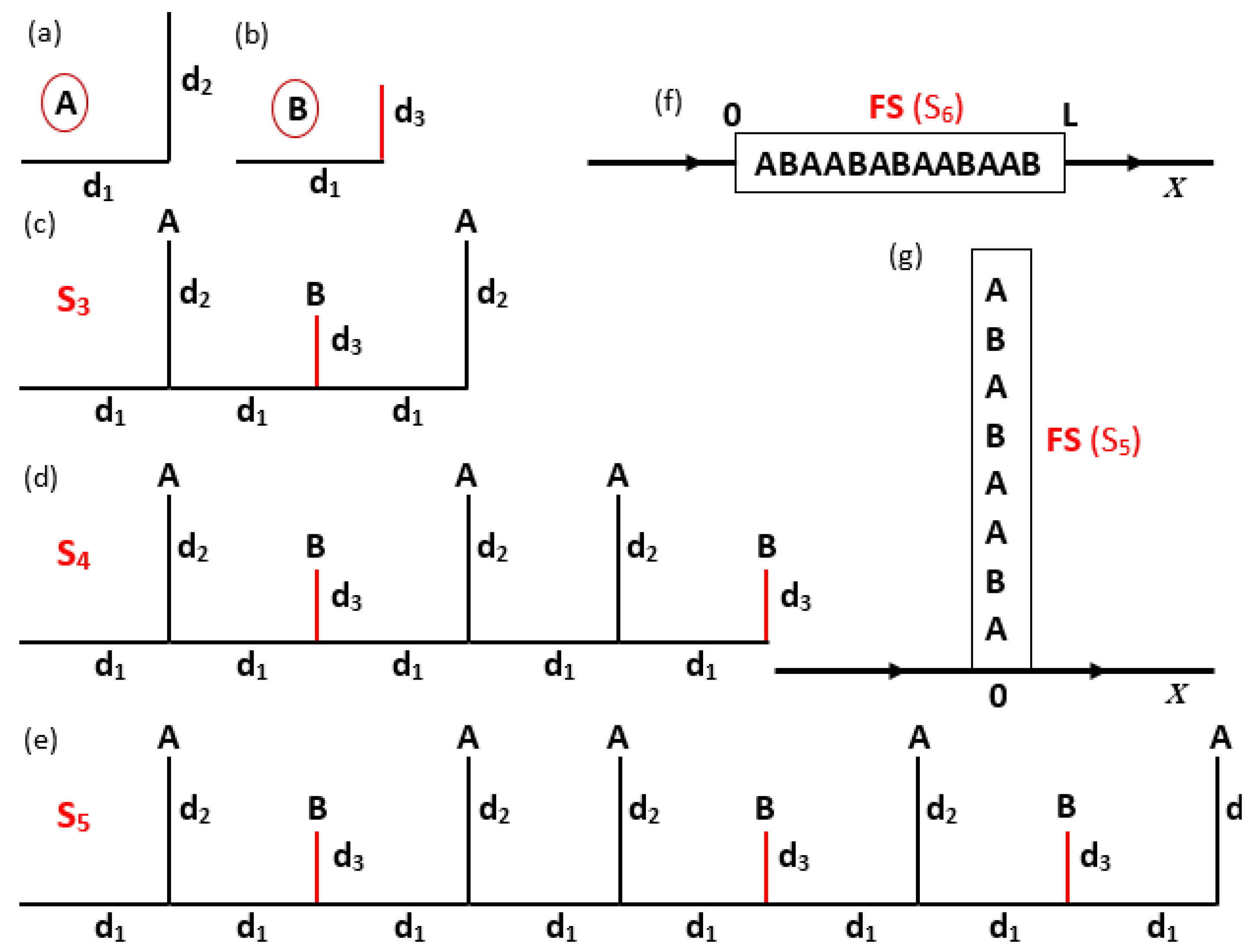
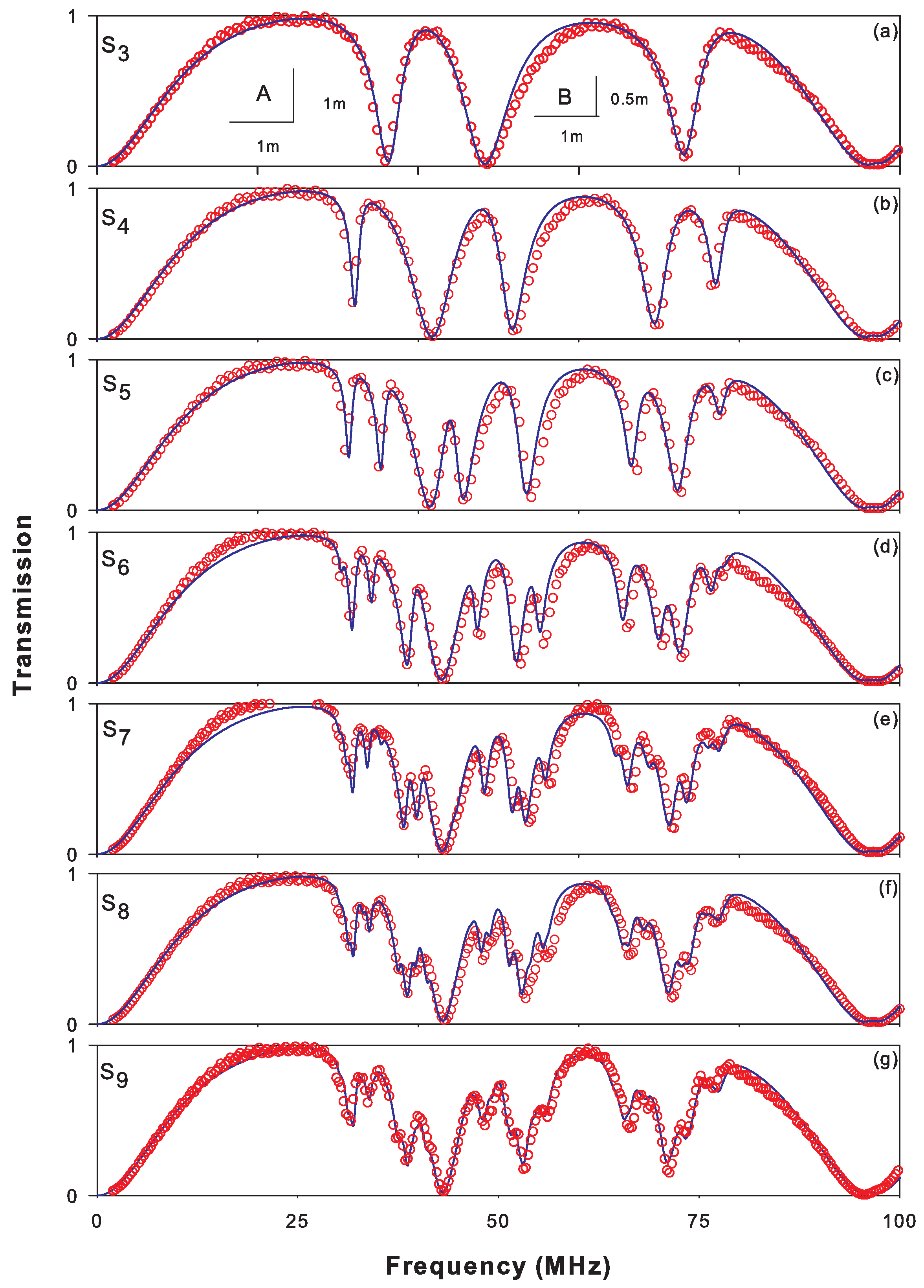
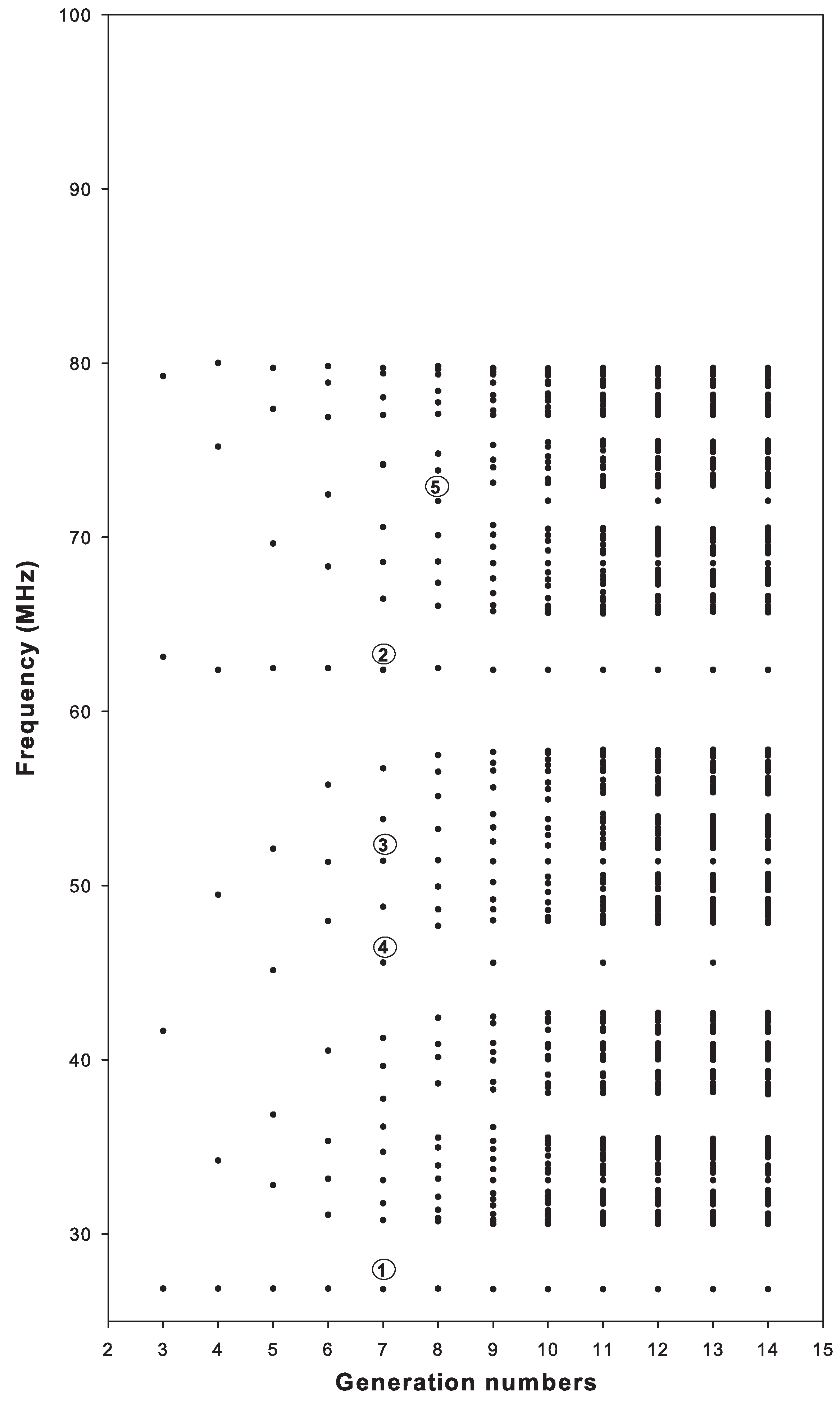
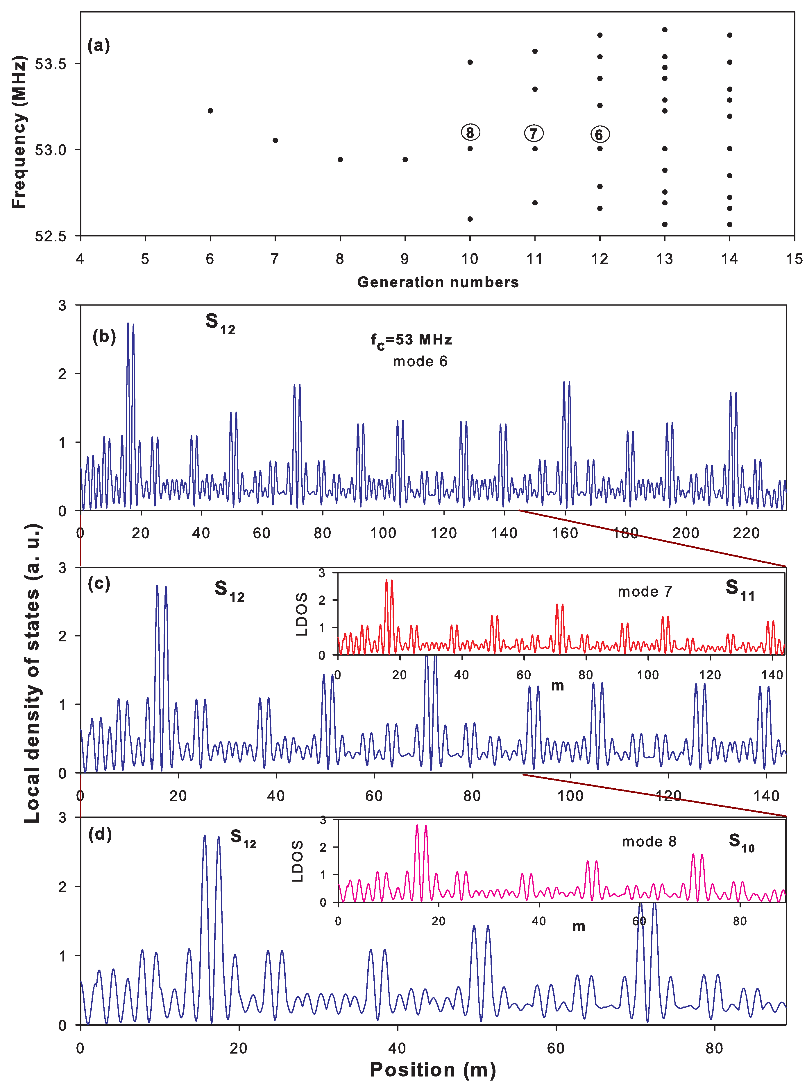
4.2. Horizontal Fibonacci Sequence: Scaling Law

In this subsection, we will discuss the properties of wave propagation and localization in a Fibonacci sequence sandwiched horizontally between two semi-infinite waveguides (Figure 1f). To our knowledge, neither theoretical nor experimental studies have been performed on photonic crystals using such quasi-periodic systems. Figure 3b–g give the transmission coefficient versus the frequency for the generations $S_4$, $S_5$, $S_6$, $S_7$, $S_8$ and $S_9$ composed of 5, 8, 13, 21, 34 and 55 blocks, respectively. Solid, dashed and open circles lines have the same meaning as defined in Figure 2. In this figure, one can distinguish two regions of frequencies: the regions where the transmission presents clear dips as the generation number increases, which correspond to the forbidden bands, and the regions where the transmission is more pronounced, which corresponds to the allowed bands. From these results, it can be derived that the transmission for the Fibonacci structures (Figure 3b–g) has more than one gap (transmission dip) with respect to the transmission spectrum of the periodic system composed by an alternate repetition of A and B blocks (Figure 3a), especially for increasing generations of FS (Figure 3c–g). This phenomenon is the result of the fragmentation of the spectrum (subdivision of the bands) when the generation number increases. An interesting result illustrated in Figure 3b–g is the occurrence of new characteristics around the frequency $f_c=53$ MHz at the center of the gap associated with the periodic structure (Figure 3a). These resonances exhibit a certain order of repetition which is a typical characteristic of Fibonacci structures. This property, known as the scaling law [36,64], has been considered as a sign of localization of the waves in Fibonacci systems. In the frame of a theoretical investigation of electronic transport in periodic and quasiperiodic mesoscopic structures with stubs and using the beautiful ’trace map’ method introduced by Kohmoto et al. [36], Jin et al. [64] demonstrated that the scaling behavior of the transmission spectra in Fibonacci stubbed structures is characterized by the scaling factor

$$F=\sqrt{1+4{(1+I)}^2}+2(1+I),$$

(15)

where I is an invariant that remains unchanged at each step of the recursive repetition [36,64]. It was demonstrated that this invariant is given by [64]

$$I=\frac{1}{4}{[cot\left(\frac{\omega d_2\sqrt{\epsilon }}{c}\right)-cot\left(\frac{\omega d_3\sqrt{\epsilon }}{c}\right)]}^2{sin}^2(\omega d_1\sqrt{\epsilon }/c).$$

(16)

Similar expressions to Equations (15) and (16) have been derived by Nomata and Horie [65] using Kohmoto-Kadanoff-Tang renormalization-group theory [79]. Furthermore, it has been demonstrated [36,64] that the self-similarity property occurs around the frequency $f_c=53$ MHz at the center of the gap of the periodic structure. This implies that the transmission coefficient should exhibit a self-similar behavior around the central frequency with $T_{j+3}=T_j$ (i.e., the transmittance is periodic every three generations) and according to a scaling factor F. For the frequency $f_c$, Equations (15) and (16) give $I=0.25$ and therefore $F\simeq 5.2$. This phenomenon is clearly depicted in the insets of Figure 3b–g near $f_c$. One can see a high similitude of the generations $S_4$–$S_7$, $S_5$–$S_8$ and $S_6$–$S_9$ with a third order periodicity and a scaling factor F (see the inset around $f_c$) as it was found theoretically by Jin et al. [64] in quantum wires with serial stubs and El Boudouti et al. [61] in Fibonacci serial loop structures. Nevertheless, it can be pointed out that due to the attenuation in the coaxial cables, the similarities between the different curves around the central gap frequency $f_c$ do not exhibit exactly the same features as it is the case in the absence of loss (see the dashed curves in Figure 3). This is particularly pronounced for higher generations. It is worth noticing that the above self-similarity between the transmission spectra requires the boundary condition E = 0 on the stub ends, otherwise one can check numerically that for the boundary condition H = 0 with the same geometrical parameters, this property is not fulfilled in all the frequency spectra.

It has been found that the localization of modes in a Fibonacci structure exhibits critical behavior within the structure [80]. Indeed, contrary to disordered systems, these modes decrease according to a power law instead of an exponential law and the localization of these modes displays the property of self-similarity [81]. In order to understand the spatial localization of the different modes in Figure 3 and Figure 4a,c illustrate the local density of states (LDOS) versus the space position x for the modes located at central gap frequency $f_c=53$ MHz for generations $S_{14}$, $S_{11}$ and $S_8$ respectively. The LDOS reflects the square modulus of the electric field inside the structure. The LDOS shows a self-similarity behavior [31,82] around the main peak every three generations as it is shown in the insets of Figure 4b,c displayed for the 11th and 8th generations respectively. These results show that the electric field around the central frequency is neither extended nor localized. This particular field localization, which is due the quasi-periodicity arrangement of the blocks A and B in the FS, has been explained by a multifractal analysis to understand the critical behavior of such modes [31,50,62,81,83].

The behavior of the modes lying at the band edges is also analyzed as shown in Figure 5 for the mode $f=68.08$ MHz in Figure 3f. The spectrum of LDOS is less regular compared to the band edge resonances occurring in the periodic structure (see the inset of Figure 5 for the mode $f=61.40$ MHz). However, band edge resonances in periodic photonic crystals are non-localized states since they propagate throughout the system and are not evanescent [31]. In contrast, the Fibonacci band edge resonances may decay via a power law due to the non-periodic character of the blocks A and B in these systems [36,84]. This kind of resonances has been shown to be useful in designing new complex cavity in 1 D photonic crystals that enables the feedback for laser action in the domain of random laser devices [85].

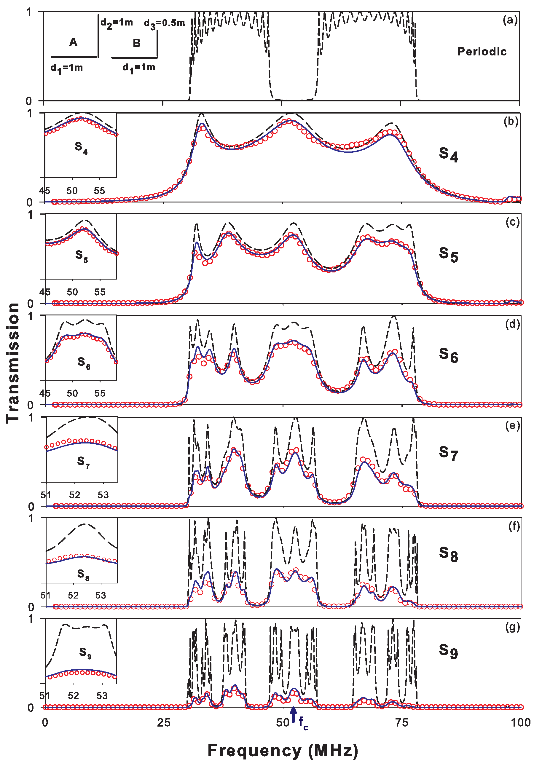
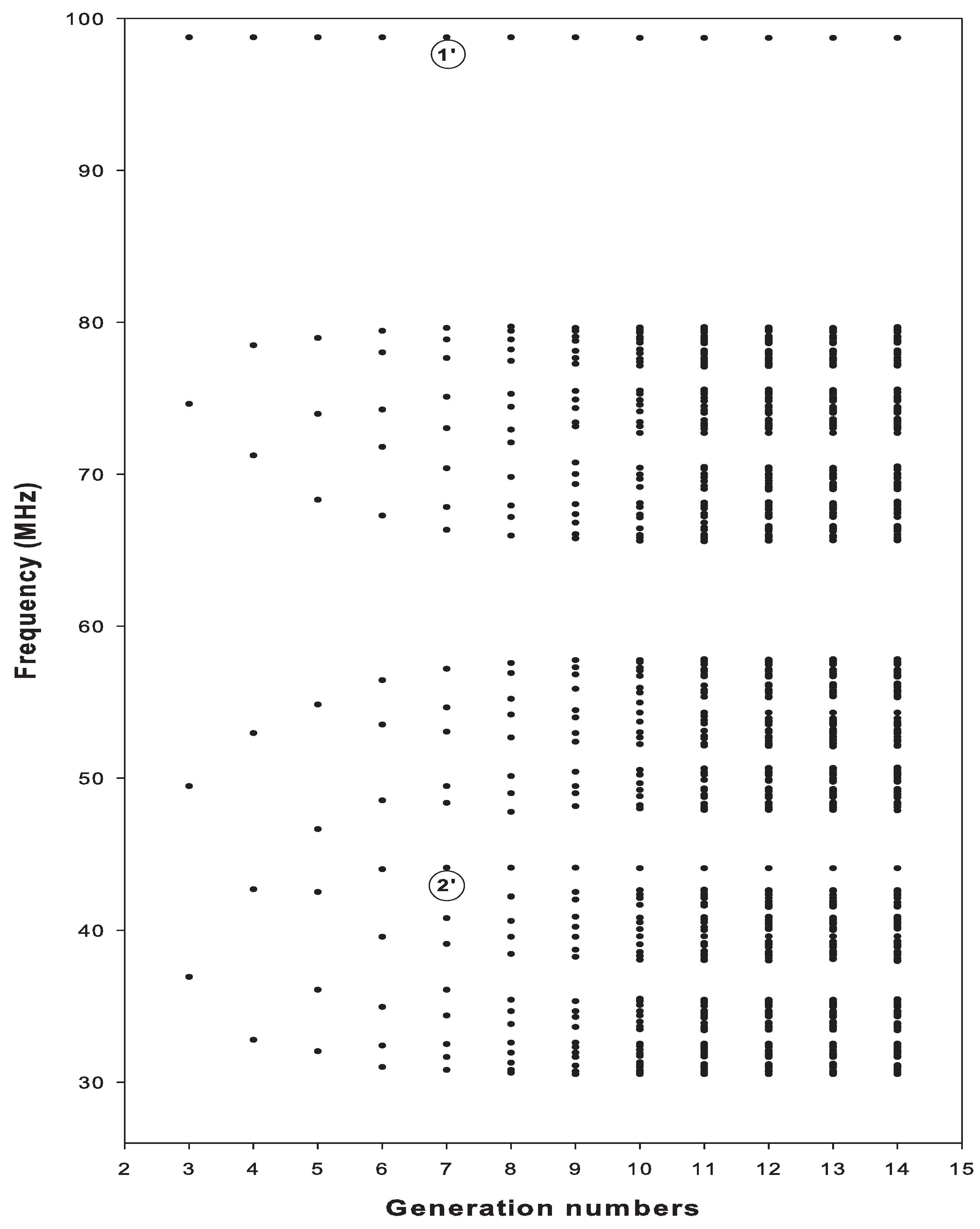
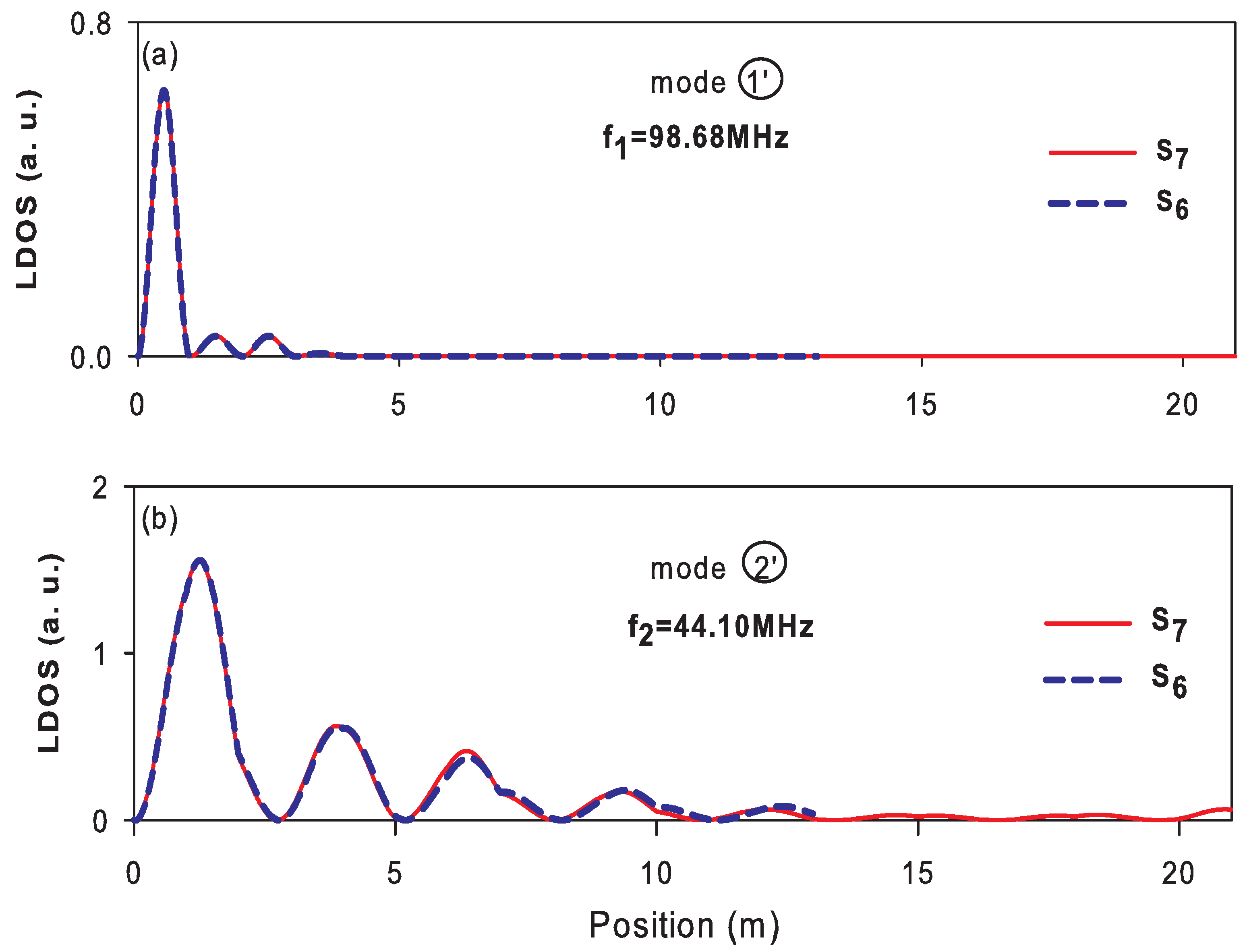
4.3. Vertical Fibonacci Sequence: Confined and Surface Modes

In the following, we will discuss the case where the Fibonacci sequences are grafted vertically to an horizontal waveguide (Figure 1g). The choice of this geometry is motivated by the fact that the maxima and minima of the transmission spectra permit to deduce all the eigenmodes of the structure [70,71]. As mentioned in Section 2, the transmission maxima occur for the eigenfrequencies of the finite FS when the boundary conditions at its both ends are perfect magnetic conductor type (i.e., vanishing magnetic field). However, the transmission minima occurs for eigenfrequencies of the finite Fibonacci sequence when the boundary conditions are perfect magnetic conductor type on the free surface of the structure and perfect electric conductor type (i.e., vanishing electric field) on the other side which will be grafted on the waveguide. The evolution of the transmission versus the frequency is displayed in Figure 6 for the generations $S_3$–$S_9$. It is shown that there are transmission oscillations between minima and maxima within the frequency range from 30 and 80 MHz. In addition, the theoretical results (solid curves) are in good agreement with the experimental ones (open circles). As predicted, these findings clearly show that the eigenmodes of the FS falling essentially inside the frequency region [30–80] MHz, where the transmission spectra of the horizontal Fibonacci structure is more pronounced (see Figure 3). The frequencies corresponding to the maxima of the transmittance (Figure 6) are reported in Figure 7 by dots for different generations. As a matter of completeness, Figure 7 displays the theoretical results for the generations $S_{10}$–$S_{14}$. The experimental spectra of these high order generations are difficult to measure as the modes become very close to each other (Figure 7). As predicted, the number of eigenmodes of a FS increases with increasing the generation number. One can notice that, apart surface modes falling in the forbidden bands at the same frequency for all generations or for one generation over two, the other modes accumulate in the allowed bands in accordance with the results in Figure 3.

To widen the scope of our findings, Figure 8 illustrates the LDOS as a function of the space position x for the surface modes labeled 1, 2, 3, 4 and 5 in Figure 7. These modes present different behaviors: the modes labeled 1, 2 and 3 in Figure 7 fall at the same frequency regardless the number of generations. Indeed, these modes are induced by the same surface terminated by block A for all generations as illustrated in Figure 8a–c, respectively. One can notice that for the modes 1 and 2 localized in primary gaps (Figure 7), the LDOS decreases rapidly far from the surface (Figure 8a,b), while for the mode 3 lying inside a secondary gap (Figure 7), the LDOS decreases less rapidly (Figure 8c). In addition, the spatial localization of these modes is independent of the generation number, as shown in Figure 8a–c for generations $S_6$ (dashed lines) and $S_7$ (solid lines). The modes denoted 4 and 5 in Figure 7 fall at the same frequency every two generations. In contrast to modes 1, 2 and 3, which are induced by the bottom surface of the FS (Figure 1g), modes 4 and 5 are generated by the top surfaces in which the terminations are not the same for odd (block A) and even (block B) generations. Consequently, the mode 4 (5) is induced by odd (even) generations, as illustrated in Figure 8d,e. Furthermore, the spatial behavior of the square modulus of the electric field of the mode lying at the central frequency $f_c=53$ MHz is displayed in Figure 9b–d. Indeed, a magnification of Figure 7 around $f_c$ (Figure 9a) shows stable modes. The behavior of the electric field of such modes are not similar to surface modes (Figure 8), but exhibit rather a self similar behavior as for the horizontal Fibonacci structure (Figure 4). This is illustrated in Figure 9b–d for the mode labeled 6 (12th generation) as compared to the modes labeled 7 and 8 for the 11th and 10th generations respectively. However, one can notice that the self-similarity occurs here every generation instead of three generations as it is the case in Figure 4, where the range on the horizontal axis is adapted for comparison to 11th and 10th FS generations.

As mentioned in Section 2, the minima of the transmittance plotted in Figure 6 give the eigenmodes of the finite FS with vanishing electric field on one side and magnetic field on the other side. These minima are reported in Figure 10 for different generations. One can notice that the eigenmodes of this system are quite different from those of the FS with vanishing magnetic field on both sides (Figure 10). Moreover, the primary and secondary gaps appear as the generation number increases and some of these gaps exhibit surface modes denoted 1${}^{\prime }$ and 2${}^{\prime }$ for all generations. These modes are induced by the short-circuited surface as illustrated by the spatial localization of the electric field displayed in Figure 11 for these two modes. One can see clearly a decrease of the LDOS (or the square modulus of the electric field) of these modes far from the surface when penetrating inside the bulk of the Fibonacci system with almost the same localization length (solid and dashed curves). The typical features of confined and surface waves in photonic Fibonacci stub structures can provide added value for technology applications and offer many solutions to various problems with respect to periodic or defected structures. Moreover, the two configurations of FS proposed here can produce multiple photonic bandgaps and different resonant peaks/dips which can be utilized as a high precision selective/rejective filter to the incident wave. Finally, it is worth mentioning that the edge modes in a Fibonacci photonic quasicrystal [73] are found quantitatively equivalent to those of the Harper model [72], showing their topological origin [74].

5. Conclusions

We have studied both theoretically and experimentally the behavior of the propagating and localization of electromagnetic modes in periodic and Fibonacci stub structures. Each block constituting the Fibonacci (or periodic) structure is formed by an horizontal segment and a vertical stub. Different features of the transmission spectra and confined modes in Fibonacci structures inserted horizontally between two semi-infinite waveguides or grafted vertically along a guide have been analyzed. It was shown through an analysis of the transmission spectra of the horizontal structure that such systems exhibit the self-similar behavior of order three around the central gap frequency of the periodic structure and the fragmentation of the frequency spectrum when the generation number increases. Also, the spatial localization of the different modes around the central frequency shows a self-similar behavior of order three.

Furthermore, the behavior of the eigenmodes of the FS with different boundary conditions on its both extremities has been studied. Also, as predicted, the number of eigenmodes of the FS increases with increasing the generation number. In addition to the allowed modes, it was shown in the case of a FS with H = 0 boundary conditions on both sides, the existence of other modes induced by one surface which fall at the same frequency for different generations, their spatial localization being independent of the generation number. Moreover, the modes generated by the other surface in which the terminations are not the same for odd and even generations, fall at the same frequency every two generations. These findings are different from those of the FS with H = 0 on one side and E = 0 on the other side, where the surface modes appear only on the termination with E = 0. The experiments are performed by using standard coaxial cables in the radio frequency domain. These results are in good agreement with the 1D theoretical model based on the Green’s function approach.

Despite the difference of scale between coaxial cables and usual photonic crystals, the physical phenomena reported here, such as scaling law, confined and surface modes, can be obtained in their analogues photonic crystals. In particular, by using appropriate scales, the geometries presented in this paper can be transposed to micro-resonators operating in microwave and optical ranges, see, for example, our recent papers on demultiplexer circuits based on coaxial cables [86] and plasmonic waveguides [87].

References

1. Shechtman, D.; Bletch, I.; Gratias, D.; Cahn, J.W. Metallic phase with long-range orientational order and no translational symmetry. Phys. Rev. Lett. 1984, 53, 1951. [Google Scholar] [CrossRef] [Green Version]
2. Levine, D.; Steinhardt, P.J. Quasicrystals: A new class of ordered structures. Phys. Rev. Lett. 1984, 53, 2477. [Google Scholar] [CrossRef] [Green Version]
3. Li, C.; Ji, A.; Cao, Z. Stressed Fibonacci spiral patterns of definite chirality. Appl. Phys. Lett. 2007, 90, 164102. [Google Scholar] [CrossRef] [Green Version]
4. Maciá, E. Aperiodic Structures in Condensed Matter: Fundamentals and Applications; CRC Press: Boca Raton, FL, USA, 2009. [Google Scholar]
5. Vardeny, Z.V.; Nahata, A.; Agrawal, A. Optics of photonic quasicrystal. Nat. Photonics 2013, 7, 177. [Google Scholar] [CrossRef]
6. Negro, L.D. Optics of Aperiodic Structures: Fundamentals and Device Applications; Pan Stanford Publishing: Singapore; CRC Press: Boca Raton, FL, USA, 2013. [Google Scholar]
7. Zhao, Y.F.; Wang, Z.M.; Jiang, Z.J.; Chen, X.; Yue, C.X.; Wang, J.Z.; Liu, J.J. Add-drop filter with compound structures of photonic crystal and photonic quasicrysta. J. Infrared Millim. Waves 2017, 36, 342–348. [Google Scholar]
8. Ren, J.; Sun, X.; Wang, S. A narrowband filter based on 2D 8-fold photonic quasicrystal. Superlattices Microstruct. 2018, 116, 221. [Google Scholar] [CrossRef]
9. Trabelsi, Y.; Ali, N.B.; Elhawil, A.; Krishnamurthy, R.; Kanzari, M.; Amiri, I.S.; Yupapin, P. Design of structural gigahertz multichanneled filter by using generalized Fibonacci superconducting photonic quasicrystals. Results Phys. 2019, 13, 102343. [Google Scholar] [CrossRef]
10. Liu, E.; Tan, W.; Yan, B.; Xie, J.L.; Ge, R.; Liu, J.J. Broadband ultra-flattened dispersion, ultra-low confinement loss and large effective mode area in an octagonal photonic quasi-crystal fiber. J. Opt. Soc. Am. A 2018, 35, 431. [Google Scholar] [CrossRef] [PubMed]
11. Yan, B.; Wang, A.; Liu, E.; Tan, W.; Xie, J.; Ge, R.; Liu, J. Polarization filtering in the visible wavelength range using surface plasmon resonance and a sunflower-type photonic quasi-crystal fiber. J. Phys. D Appl. Phys. 2018, 51, 155105. [Google Scholar] [CrossRef]
12. Vitiello, M.S.; Nobile, M.; Ronzani, A.; Tredicucci, A.; Castellano, F.; Talora, V.; Li, L.; Linfield, E.H.; Davies, A.G. Photonic quasi-crystal terahertz lasers. Nat. Commun. 2014, 5, 5884. [Google Scholar] [CrossRef] [Green Version]
13. Notomi, M.; Suzuki, H.; Tamamura, T.; Edagawa, K. Lasing action due to the two-dimensional quasiperiodicity of photonic quasicrystals with a Penrose lattic. Phys. Rev. Lett. 2004, 92, 123906. [Google Scholar] [CrossRef] [PubMed]
14. Mahler, L.; Tredicucci, A.; Beltram, F.; Walther, C.; Faist, J.; Beere, H.E.; Ritchie, D.A.; Wiersma, D.S. Quasi-periodic distributed feedback laser. Nat. Photonics 2010, 4, 165. [Google Scholar] [CrossRef]
15. Ren, J.; Sun, X.; Wang, S. A low threshold nanocavity in a two-dimensional 12-fold photonic quasicrysta. Opt. Laser Technol. 2018, 101, 42. [Google Scholar] [CrossRef]
16. Chen, H.; Zhao, J.; Fang, Z.; An, D.; Zhao, X. Visible light metasurfaces assembled by quasiperiodic dendritic cluster sets. Adv. Mater. Interfaces 2019, 6, 1801834. [Google Scholar] [CrossRef]
17. Liu, J.J.; Fan, Z.G. Size limits for focusing of two-dimensional photonic quasicrystal lenses. IEEE Photonics Technol. Lett. 2018, 30, 1001. [Google Scholar] [CrossRef]
18. Wang, X.; Zhou, L.; Zhao, T.; Liu, X.; Feng, S.; Chen, X.; Guo, H.; Li, C.; Wang, Y. High-sensitivity quasi-periodic photonic crystal biosensor based on multiple defective modes. Appl. Opt. 2019, 58, 2860. [Google Scholar] [CrossRef]
19. Lee, S.Y.; Amsden, J.J.; Boriskina, S.V.; Gopinath, A.; Mitropolous, A.; Kaplan, D.L.; Omenetto, F.G.; Negro, L.D. Spatial and spectral detection of protein monolayers with deterministic aperiodic arrays of metal nanoparticles. Proc. Natl. Acad. Sci. USA 2010, 107, 12086. [Google Scholar] [CrossRef] [PubMed] [Green Version]
20. Mauriz, P.W.; Vasconcelos, M.S.; Albuquerque, E.L. Optical transmission spectra in symmetrical Fibonacci photonic multilayers. Phys. Lett. A 2009, 373, 496. [Google Scholar] [CrossRef]
21. Negro, L.D.; Yi, J.H.; Nguyen, V.; Michel, Y.Y.J.; Kimerling, L.C. Spectrally enhanced light emission from aperiodic photonic structures. Appl. Phys. Lett. 2005, 86, 261905. [Google Scholar] [CrossRef]
22. Boriskina, S.V.; Gopinath, A.; Negro, L.D. Optical gap formation and localization properties of optical modes in deterministic aperiodic photonic structures. Opt. Express 2008, 16, 18813. [Google Scholar] [CrossRef]
23. Hiltunen, M.; Negro, L.D.; Ning-Ning, F.; Kimerling, L.C.; Michel, J. Modeling of aperiodic fractal waveguide structures for multifrequency light transport. J. Light. Technol. 2007, 25, 1841. [Google Scholar] [CrossRef] [Green Version]
24. Zotov, N.; Feydt, J.; Walther, T.; Ludwig, A. Structure of PtFe/Fe double-period multilayers investigated by X-ray diffraction, reflectivity, diffuse scattering and TEM. Appl. Surf. Sci. 2006, 253, 128. [Google Scholar] [CrossRef]
25. Lambropoulos, K.; Simserides, C. Periodic, quasiperiodic, fractal, Kolakoski, and random binary polymers: Energy structure and carrier transport. Phys. Rev. E 2019, 99, 032415. [Google Scholar] [CrossRef] [Green Version]
26. Esaki, K.; Sato, M.; Kohmoto, M. Wave propagation through Cantor-set media: Chaos, scaling, and fractal structures. Phys. Rev. E 2009, 79, 056226. [Google Scholar] [CrossRef] [Green Version]
27. Sakaguchi, H.; Ogawana, T. Scaling laws of reflection coefficients of quantum waves at a Cantor-like potential. Phys. Rev. E 2017, 95, 032214. [Google Scholar] [CrossRef]
28. Ogawana, T.; Sakaguchi, H. Transmission coefficient from generalized Cantor-like potentials and its multifractality. Phys. Rev. E 2018, 97, 012205. [Google Scholar] [CrossRef]
29. Albuquerque, E.L.; Cottam, M.G. Polaritons in Periodic and Quasiperiodic Structures; Elsevier: Amsterdam, The Netherlands, 2004. [Google Scholar]
30. Merlin, R.; Bajema, K.; Clarke, R.; Juang, F.Y.; Bhattacharya, P.K. Quasiperiodic GaAs-AlAs Heterostructures. Phys. Rev. Lett. 1985, 55, 1768. [Google Scholar] [CrossRef]
31. Kohmoto, M.; Sutherland, B.; Tang, C. Critical wave functions and a Cantor-set spectrum of a one-dimensional quasicrystal model. Phys. Rev. B 1987, 35, 1020. [Google Scholar] [CrossRef] [Green Version]
32. Tamura, S.; Wolfe, J.P. Acoustic-phonon transmission in quasiperiodic superlattices. Phys. Rev. B 1987, 36, 3491. [Google Scholar] [CrossRef]
33. Aynaou, H.; El Boudouti, E.H.; Djafari-Rouhani, B.; Akjouj, A.; Velasco, V.R. Propagation and localization of acoustic waves in Fibonacci phononic circuits. J. Phys. Condens. Matter 2005, 17, 4245. [Google Scholar] [CrossRef]
34. Aynaou, H.; Velasco, V.R.; Nougaoui, A.; El Boudouti, E.H.; Bria, D. Properties of elastic waves in quasiregular structures with planar defects. Superlattices Microstruct. 2002, 32, 35. [Google Scholar] [CrossRef]
35. Ma, B.; Liu, T.; Liu, W.; Xue, J.; Tao, Z. Non-Bragg Bands in Acoustic Quasi-Periodic Fibonacci Waveguides. Phys. Status Solidi 2019, 13, 1900203. [Google Scholar] [CrossRef]
36. Kohmoto, M.; Sutherland, B.; Iguchi, K. Localization of optics: Quasiperiodic media. Phys. Rev. Lett. 1987, 58, 2436. [Google Scholar] [CrossRef]
37. Hattori, T.; Tsurumachi, N.; Kawato, S.; Nakatsuka, H. Photonic dispersion relation in a one-dimensional quasicrystal. Phys. Rev. B 1994, 50, 4220. [Google Scholar] [CrossRef]
38. Costa, C.H.O.; Vasconcelos, M.S.; Albuquerque, E.L. Band structures of exchange spin waves in one-dimensional bi-component magnonic crystals. J. Appl. Phys. 2011, 109, 07D319. [Google Scholar] [CrossRef]
39. Nguyen, T.D.; Nahata, A.; Vardeny, Z.V. Measurement of surface plasmon correlation length differences using Fibonacci deterministic hole arrays. Opt. Express 2012, 20, 15222. [Google Scholar] [CrossRef] [PubMed]
40. Dong, J.W.; Fung, K.; Chan, C.; Wang, H.Z. Localization characteristics of two-dimensional quasicrystals consisting of metal nanoparticles. Phys. Rev. B 2009, 80, 155118. [Google Scholar] [CrossRef] [Green Version]
41. Dallapiccola, R.; Gopinath, A.; Stellacci, F.; Negro, L.D. Quasi-periodic distribution of plasmon modes in two-dimensional Fibonacci arrays of metal nanoparticles. Opt. Express 2008, 16, 5544. [Google Scholar] [CrossRef] [PubMed]
42. Bajema, K.; Merlin, R. Raman scattering by acoustic phonons in Fibonacci GaAs-AIAs superlattices. Phys. Rev. B 1987, 36, 4555. [Google Scholar] [CrossRef]
43. Hurley, D.C.; Tamura, S.; Wolfe, J.P.; Ploog, K.; Nagle, J. Angular dependence of phonon transmission through a Fibonacci superlattice. Phys. Rev. B 1988, 37, 8829. [Google Scholar] [CrossRef]
44. Maciá, E.; Domínguez-Adame, F. Electrons, Phonons and Excitons in Low Dimensional Aperiodic Systems; Editorial Complutense: Madrid, Sapin, 2000. [Google Scholar]
45. King, P.D.C.; Cox, T.J. Acoustic band gaps in periodically and quasiperiodically modulated waveguides. J. Appl. Phys. 2007, 102, 014902. [Google Scholar] [CrossRef]
46. Bellingeri, M.; Chiasera, A.; Kriegel, I.; Scotognella, F. Optical properties of periodic, quasi-periodic, and disordered one-dimensional photonic structures. Opt. Mat. 2017, 72, 403. [Google Scholar] [CrossRef] [Green Version]
47. Gellermann, W.; Kohmoto, M.; Sutherland, B.; Taylor, P.C. Localization of light waves in Fibonacci dielectric multilayers. Phys. Rev. Lett. 1994, 72, 633. [Google Scholar] [CrossRef]
48. Pelster, R.; Gasparian, V.; Nimtz, G. Propagation of plane waves and of waveguide modes in quasiperiodic dielectric heterostructures. Phys. Rev. E 1997, 55, 7645. [Google Scholar] [CrossRef] [Green Version]
49. Peng, R.W.; Liu, Y.M.; Huang, X.Q.; Qin, F.; Wang, M.; Hu, A.; Jiang, S.S.; Feng, D.; Ouyang, L.Z.; Zou, J. Dimerlike positional correlation and resonant transmission of electromagnetic waves in aperiodic dielectric multilayers. Phys. Rev. B 2004, 69, 165109. [Google Scholar] [CrossRef] [Green Version]
50. Ghulinyan, M.; Oton, C.J.; Negro, L.D.; Pavesi, L.; Sapienza, R.; Colocci, M.; Wiersma, D.S. Light-pulse propagation in Fibonacci quasicrystals. Phys. Rev. B 2005, 71, 094204. [Google Scholar] [CrossRef] [Green Version]
51. Peng, R.W.; Wang, M.; Hu, A.; Jiang, S.S.; Jin, G.J.; Feng, D. Photonic localization in one-dimensional k-component Fibonacci structures. Phys. Rev. B 1998, 57. [Google Scholar] [CrossRef]
52. Sibilia, C.; Nefedov, I.S.; Scolara, M.; Berlotti, M. Electromagnetic mode density for finite quasi-periodic structures. J. Opt. Soc. Am. B 1998, 15, 1947. [Google Scholar] [CrossRef]
53. Huang, X.; Wang, Y.; Gong, C. Numerical investigation of light-wave localization in optical Fibonacci superlattices with symmetric internal structure. J. Phys. Condens. Matter 1999, 11, 7645. [Google Scholar] [CrossRef]
54. Liu, N.H. Propagation of light waves in Thue-Morse dielectric multilayers. Phys. Rev. B 1997, 55, 3543. [Google Scholar] [CrossRef]
55. Lavrinenko, A.V.; Zhukovsky, S.V.; Sandmirski, K.S.; Gaponenko, S.V. Propagation of classical waves in nonperiodic media: Scaling properties of an optical Cantor filter. Phys. Rev. E 2002, 65, 036621. [Google Scholar] [CrossRef] [Green Version]
56. Macia, E. Exploiting quasiperiodic order in the design of optical devices. Phys. Rev. B 2001, 63, 205421. [Google Scholar] [CrossRef] [Green Version]
57. Lusk, D.; Abdulhalim, I.; Placido, F. Omnidirectional reflection from Fibonacci quasi-periodic one-dimensional photonic crystal. Opt. Commun. 2001, 198, 273. [Google Scholar] [CrossRef]
58. Segovia-Chaves, F.; Vinck-Posada, H. Transmittance spectrum of a superconductor-semiconductor quasiperiodic one-dimensional photonic crystal. Physica C 2019, 563, 10. [Google Scholar] [CrossRef]
59. Elsayed, H.A.; Abadla, M.M. Transmission investigation of one-dimensional Fibonacci-based quasi-periodic photonic crystals including nanocomposite material and plasma. Phys. Scr. 2020, 95, 035504. [Google Scholar] [CrossRef]
60. Aynaou, H.; El Boudouti, E.H.; El Hassouani, Y.; Akjouj, A.; Djafari-Rouhani, B.; Vasseur, J.; Benomar, A.; Velasco, V.R. Propagation and localization of electromagnetic waves in quasiperiodic serial loop structures. Phys. Rev. E 2005, 72, 056601. [Google Scholar] [CrossRef]
61. El Boudouti, E.H.; El Hassouani, Y.; Aynaou, H.; Djafari-Rouhani, B.; Akjouj, A.; Velasco, V.R. Electromagnetic wave propagation in quasi-periodic photonic circuits. J. Phys. Condens. Matter 2007, 19, 246217. [Google Scholar] [CrossRef] [PubMed]
62. El Hassouani, Y.; Aynaou, H.; El Boudouti, E.H.; Djafari-Rouhani, B.; Akjouj, A.; Velasco, V.R. Surface electromagnetic waves in Fibonacci superlattices: Theoretical and experimental results. Phys. Rev. B 2006, 74, 035314. [Google Scholar] [CrossRef]
63. Sánchez-Lopez, M.M.; Sánchez Mero no, A.; Arias, J.; Davis, J.A.; Moreno, I. Observation of superluminal and negative group velocities in a Mach-Zehnder interferometer. Appl. Phys. Lett. 2008, 93, 074102. [Google Scholar] [CrossRef]
64. Jin, G.J.; Wang, Z.D.; Hu, A.; Jiang, S.S. Quantum waveguide theory of serial stub structures. J. Appl. Phys. 1999, 85, 1597. [Google Scholar] [CrossRef] [Green Version]
65. Nomata, A.; Horie, S. Self-similarity appearance conditions for electronic transmission probability and Landauer resistance in a Fibonacci array of T stubs. Phys. Rev. B 2007, 76, 235113. [Google Scholar] [CrossRef]
66. Chattopadhyay, S.; Chakrabarti, A. Electronic transmission in quasiperiodic serial stub structures. J. Phys. Condens. Matter 2004, 16, 313. [Google Scholar] [CrossRef]
67. Vasseur, J.O.; Akjouj, A.; Djafari-Rouhani, B.; Dobrzynski, L.; El Boudouti, E.H. Photon, electron, magnon, phonon and plasmon mono-mode circuits. Surf. Sci. Rep. 2004, 54, 1. [Google Scholar] [CrossRef]
68. Dobrzynski, L.; Akjouj, A.; Djafari-Rouhani, B.; Vasseur, J.O.; Zemmouri, J. Giant gaps in photonic band structures. Phys. Rev. B 1998, 57, R9388. [Google Scholar] [CrossRef]
69. Vasseur, J.O.; Djafari-Rouhani, B.; Dobrzynski, L.; Akjouj, A.; Zemmouri, J. Defect modes in one-dimensional comblike photonic waveguides. Phys. Rev. B 1999, 49, 13446. [Google Scholar] [CrossRef]
70. El Boudouti, E.H.; El Hassouani, Y.; Djafari-Rouhani, B.; Aynaou, H. Two types of modes in finite size one-dimensional coaxial photonic crystals: General rules and experimental evidence. Phys. Rev. E 2007, 76, 026607. [Google Scholar] [CrossRef]
71. Djafari-Rouhani, B.; El Boudouti, E.H.; Akjouj, A.; Dobrzynski, L.; Vasseur, J.O.; Mir, A.; Fettouhi, N.; Zemmouri, J. Surface states in one-dimensional photonic band gap structures. Vacuum 2001, 63, 177. [Google Scholar] [CrossRef]
72. Harper, P.G. Single Band Motion of Conduction Electrons in a Uniform Magnetic Field. Proc. Phys. Soc. Lond. Sect. A 1955, 68, 874. [Google Scholar] [CrossRef]
73. Kraus, Y.E.; Zilberberg, O. Topological equivalence between the Fibonacci quasicrystal and the Harper model. Phys. Rev. Lett. 2012, 109, 116404. [Google Scholar] [CrossRef] [PubMed] [Green Version]
74. Verbin, M.; Zilberberg, O.; Lahini, Y.; Kraus, Y.E.; Silberberg, Y. Topological pumping over a photonic Fibonacci quasicrystal. Phys. Rev. B 2015, 91, 064201. [Google Scholar] [CrossRef] [Green Version]
75. Dobrzynski, L. Interface response theory of continuous composite systems. Surf. Sci. Rep. 1990, 11, 139. [Google Scholar] [CrossRef]
76. Wadell, B.C. Transmission Line Design Handbook; Artech House, Inc.: Norwood, MA, USA, 1991; Chapter 3. [Google Scholar]
77. Mouadili, A.; El Boudouti, E.H.; Soltani, A.; Talbi, A.; Djafari-Rouhani, B.; Akjouj, A.; Haddadi, K. Electromagnetically induced absorption in detuned stub waveguides: A simple analytical and experimental model. J. Phys. Condens. Matter 2014, 26, 505901. [Google Scholar] [CrossRef]
78. Khattou, S.; Amrani, M.; Mouadili, A.; El Boudouti, E.H.; Talbi, A.; Akjouj, A.; Djafari-Rouhan, B. Comparison of density of states and scattering parameters in coaxial photonic crystals: Theory and experiment. Phys. Rev. B 2020, 102, 165310. [Google Scholar] [CrossRef]
79. Kohmoto, M.; Kadanoff, L.P.; Tang, C. Localization problem in one dimension: Mapping and escape. Phys. Rev. Lett. 1983, 50, 1870. [Google Scholar] [CrossRef]
80. Macia, E.; Dominguez-Adame, F. Physical nature of critical wave functions in Fibonacci systems. Phys. Rev. Lett. 1996, 76, 2957. [Google Scholar] [CrossRef] [Green Version]
81. Fijiwara, T.; Komoto, M.; Tokihito, T. Multifractal wave functions on a Fibonacci lattice. Phys. Rev. B 1989, 40, 7413. [Google Scholar] [CrossRef]
82. Jin, D.; Jin, G. Matrix maps for substitution sequences in the biquaternion representation. Phys. Rev. B 2005, 71, 014212. [Google Scholar] [CrossRef]
83. Peng, R.W.; Jin, G.J.; Wang, M.; Hu, A.; Jiang, S.S.; Feng, D. Electronic transport in k-component Fibonacci quantum waveguides. J. Phys. Condens. Matter 2000, 12, 5701. [Google Scholar] [CrossRef]
84. Negro, L.D.; Oton, C.J.; Gaburro, Z.; Pavesi, L.; Johnson, P.; Lagendijk, A.; Righini, R.; Colocci, M.; Wiersma, D.S. Light transport through the band-edge states of Fibonacci quasicrystals. Phys. Rev. Lett. 2003, 90, 055501. [Google Scholar] [CrossRef]
85. Wiersma, D.; Sapienza, R.; Mujumdar, S.; Colocci, M.; Ghulinyan, M.; Pavesi, L. Optics of nanostructured dielectrics. J. Opt. A Pure Appl. Opt. 2005, 7, S190. [Google Scholar] [CrossRef]
86. Mouadili, A.; El Boudouti, E.H.; Soltani, A.; Talbi, A.; Haddadi, K.; Akjouj, A.; Djafari-Rouhani, B. Photonic demultiplexer based on electromagnetically induced transparency resonances. J. Phys. D Appl. Phys. 2018, 52, 075101. [Google Scholar] [CrossRef]
87. Amrani, M.; Khattou, S.; Noual, A.; El Boudouti, E.H.; Djafari-Rouhani, B. Plasmonic Demultiplexer Based on Induced Transparency Resonances: Analytical and Numerical Study. Lect. Notes Electr. Eng. 2020, 681, 239. [Google Scholar]
Figure 1. Schematic representation of blocks A and B constituting the Fibonacci structure. (a) The block A consists of a horizontal coaxial cable of length d 1 combined with another identical vertical stub of length ( d 2 = d 1 ). (b) The Block B is similar to the block A but with the length of the vertical stub of length d 3 = d 2 / 2 . All cables are characterized by the same impedance Z. (ce) give the shape of the Fibonacci sequences S 3 , S 4 and S 5 respectively. (f) A finite Fibonacci structure (6th generation) inserted horizontally between two semi-infinite waveguides. (g) A finite Fibonacci structure (5th generation) grafted vertically along a waveguide.
Applsci 10 07767 g001
Figure 2. (a,i) Dispersion curves of the periodic structures composed of only B or only A blocks respectively. (bh): Variation of the transmittance versus the frequency for different finite structures composed of 13 blocks A and B. (e) Transmission spectrum for generation S 6 of the Fibonacci structure. The solid (dashed) curves represent the theoretical results with (without) dissipation, whereas open circles correspond to the experimental data.
Applsci 10 07767 g002
Figure 3. Theoretical (solid lines) and experimental (open circles) evolution of the transmission coefficients versus the frequency for different structures. The dashed curves in (ag) are the theoretical curves when the absorption is not taken into account. The inset of (a) corresponds to the schematic illustration of blocks A and B constituting the systems. (a) The periodic structure, (bg) generation S k (k = 4–9) of the Fibonacci structure. One can compare the scale of the frequency axis near the central frequency f c in the insets of the figures associated with the generations S 4 , S 5 , S 6 and those of S 7 , S 8 , S 9 respectively.
Applsci 10 07767 g003
Figure 4. (ac) Represent the spatial representation of the local density of states (LDOS) [in arbitrary units] of the mode lying at the central frequency f c = 53 MHz for the 14th generation. The insets of (b,c) correspond to the LDOS associated with the 11th and 8th generations at f c , respectively.
Applsci 10 07767 g004
Figure 5. The local density of states (LDOS) [in arbitrary units] as a function of the space position x of the mode located at the band edge ( f = 68.08 MHz) for the 8th generation. The inset of the figure corresponds to the LDOS associated with the periodic structure of length 34 m at f = 61.40 MHz.
Applsci 10 07767 g005
Figure 6. Theoretical (solid curves) and experimental (open circles) variations of the transmittance versus the frequency for a Fibonacci sequence inserted vertically along a waveguide (Figure 1g) for the generations S 3 S 9 .
Applsci 10 07767 g006
Figure 7. Dispersion of the eigenfrequencies (dots) of different generation numbers. The boundary conditions on both sides of the Fibonacci sequence (FS) are H = 0. One can notice the existence of primary and secondary gaps. All the discrete modes are obtained from the maxima of the transmission spectra displayed in Figure 6. The labels 1, 2, 3, 4 and 5 represent the surface modes.
Applsci 10 07767 g007
Figure 8. (ac) Spatial representation of the LDOS (in arbitrary units) of the modes labeled 1, 2, 3 in Figure 7 at f 1 = 26.85 MHz (a), f 2 = 62.10 MHz (b) and f 3 = 51.38 MHz (c) respectively. Dashed (solid) lines correspond to the 6th (7th) generation. (d,e) Same as (ac) but for the modes labeled 4 and 5 in Figure 7 at f 4 = 45.56 MHz (d) and f 5 = 71.93 MHz (e), respectively. Dashed (solid) lines correspond to the 7th (9th) and 8th (10th) generation, respectively.
Applsci 10 07767 g008
Figure 9. (a) Magnification of the FS modes around the central frequency f c = 53 MHz from Figure 7. (bd) The LDOS (in arbitrary units) as a function of the space position x at the central frequency f c for the 12th generation (mode 6) where the range on the horizontal axis is adapted for comparison to 11th and 10th FS generations. The insets of (c,d) correspond to the LDOS associated with modes 7 and 8 for the 11th and 10th generations at f c , respectively.
Applsci 10 07767 g009
Figure 10. Same as in Figure 7 but for a FS with vanishing magnetic field on the top surface of the structure and vanishing electric field on the bottom surface. Here, the discrete modes are obtained from the minima of the transmission spectra displayed in Figure 6. The labels 1 and 2 correspond to the surface modes.
Applsci 10 07767 g010
Figure 11. The LDOS (in arbitrary units) versus the space position x of the modes labeled 1 and 2 in Figure 10 at f 1 = 98.68 MHz (a) and f 2 = 44.10 MHz (b), respectively. Dashed (solid) curves correspond to the 6th (7th) generation.
Applsci 10 07767 g011
Publisher’s Note: MDPI stays neutral with regard to jurisdictional claims in published maps and institutional affiliations.