3.1. Cumulative Strain Energy Density
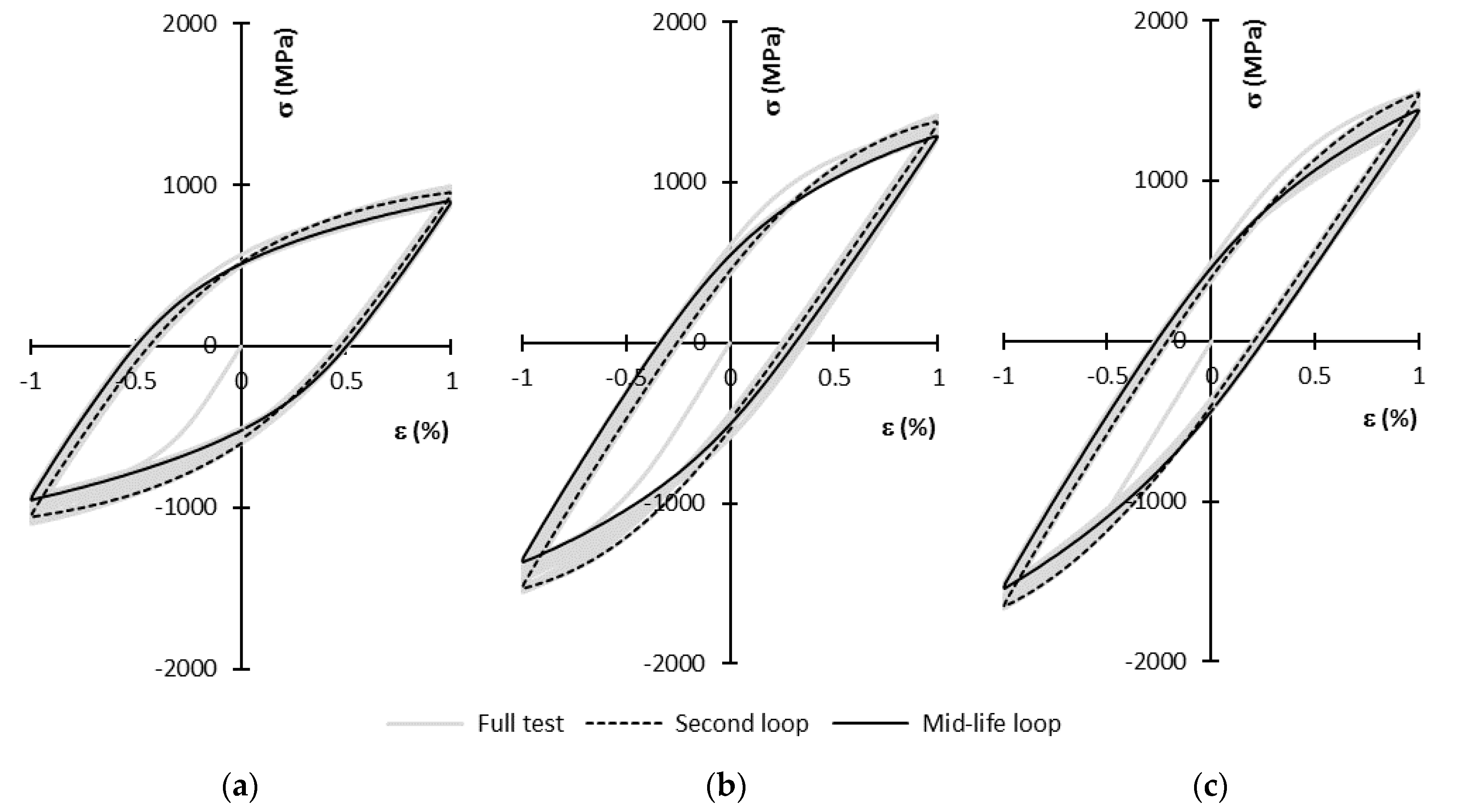
Low-cycle fatigue behavior of the tested steels under symmetrical strain-controlled conditions for a strain amplitude of 1.0% is presented in
Figure 2. As shown, the cyclic stress-strain responses were significantly different for the three materials. Overall, it was clear that the stress range associated with this strain level increased with higher Mn contents.
Moreover, irrespective of the tested steel, the shapes of the hysteresis loop changed significantly throughout the lifetime. These changes were particularly evident by comparing the second and the mid-life loops. Since the uncontrolled stress range reduced over time, the three materials exhibited a cyclic strain-softening behavior for this strain level. Literature suggests that at lower strain amplitudes Steel C maintains a similar trend, but Steel A and Steel B tend to strain-harden [
9].
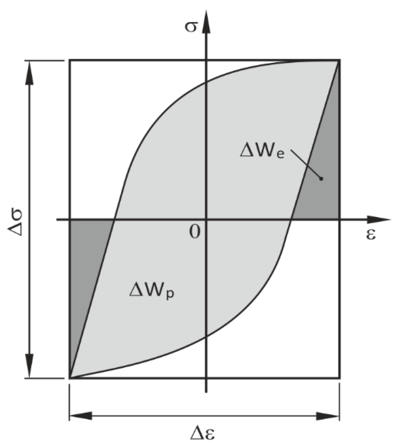
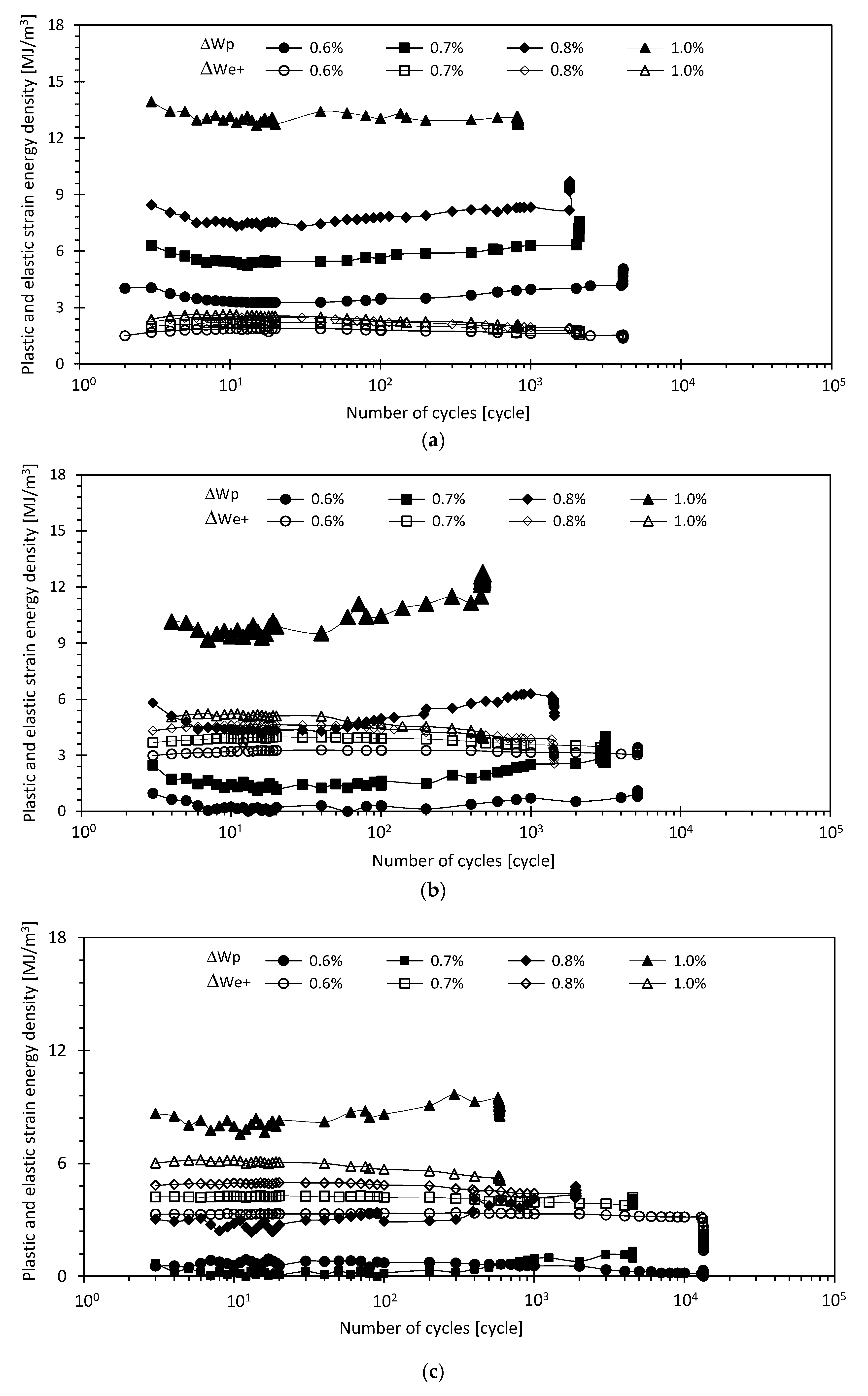
Figure 3 plots elastic and plastic strain energy densities against the number of cycles for different strain amplitudes. These variables, as can be seen, were relatively constant along time. In most cases, the curves present three main stages: a short initial period with rapid changes; a dominant saturated stage with stable values; and a final stage, close to total failure, characterized by sudden changes. As expected, elastic and plastic strain energy densities per cycle increased with strain amplitude. On the other hand, at a given strain amplitude, the values of ∆
We and ∆Wp depended on the tested steel, which agreed with the hysteresis loop shapes displayed in
Figure 1.
At a fixed value of strain amplitude, a close analysis of the results showed that plastic strain energy density per cycle was higher for steel A and tended to diminish as Mn content increased, except for ∆ε/2 = 0.6%, where steel C exhibited higher plastic strain energy density values than steel B.
As far as elastic positive strain energy density is concerned, opposite behavior was observed, i.e., the maximum values at a given strain amplitude were found for steel C. Furthermore, ∆We increased for lower contents of Mn, except for ∆ε/2 = 0.6%, where steel A had higher plastic strain energy density than steel B.
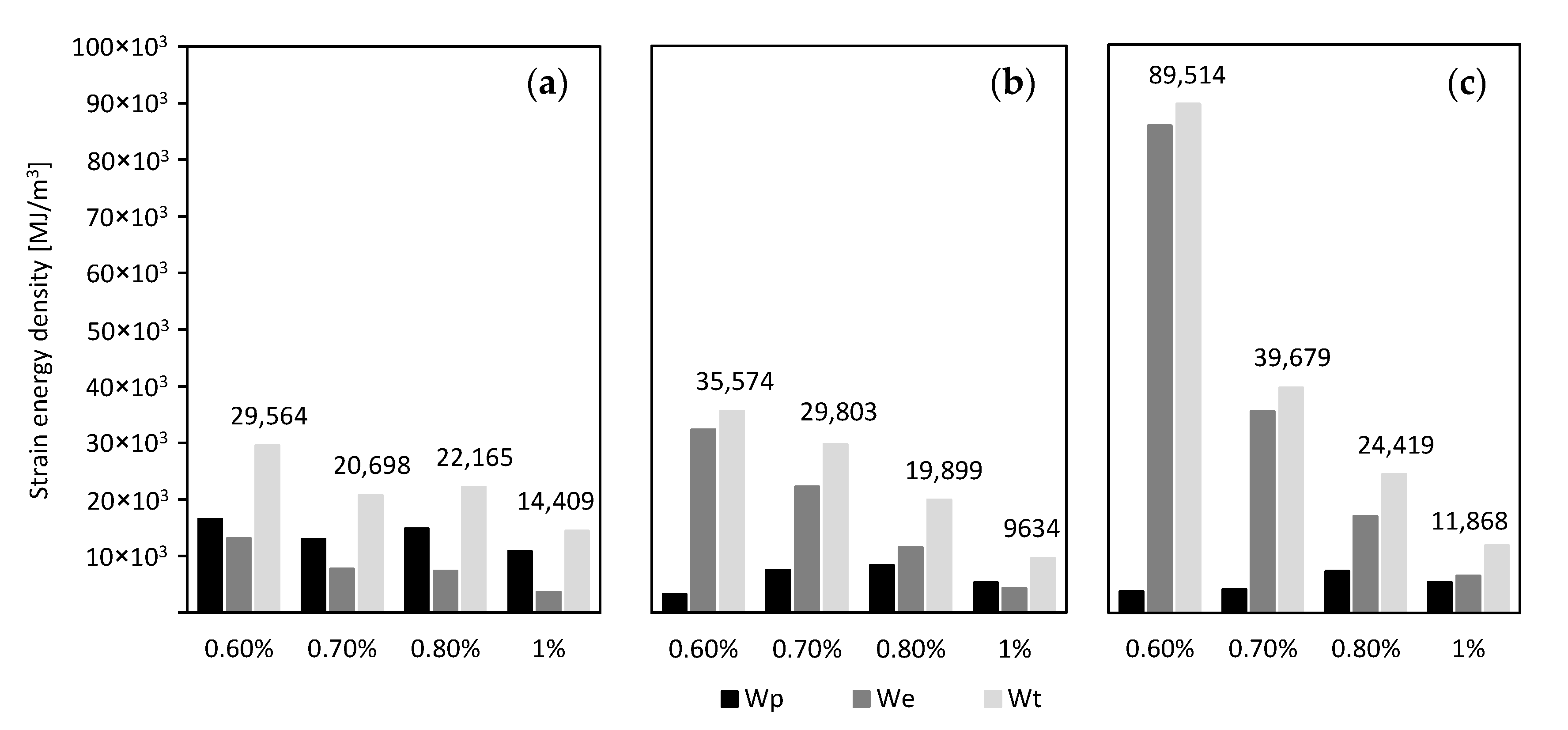
Figure 4 plots cumulative elastic (
We), plastic (Wp) and total (Wt) strain energy densities as a function of strain amplitude. The computed values of the aforementioned variables are listed in
Table 4, as well as the three components of strain energy density of the mid-life cycle, identified as ∆
We,
ML, ∆Wp,
ML and ∆Wt,
ML. At first sight, it could be concluded that steel A without Mn revealed higher plastic strain energy densities than elastic strain energy densities for all the strain amplitudes applied, showing a high fatigue toughness capability. On the contrary, the other two steels revealed higher elastic than plastic strain densities, except for steel B at a strain amplitude of 1.0%.
It is interesting to note that, at a fixed strain amplitude, steel A presented the greatest values of cumulative plastic strain energy density, similarly to plastic strain energy density per cycle; while steel C exhibited the highest cumulative elastic strain energy density, as with elastic strain energy density per cycle.
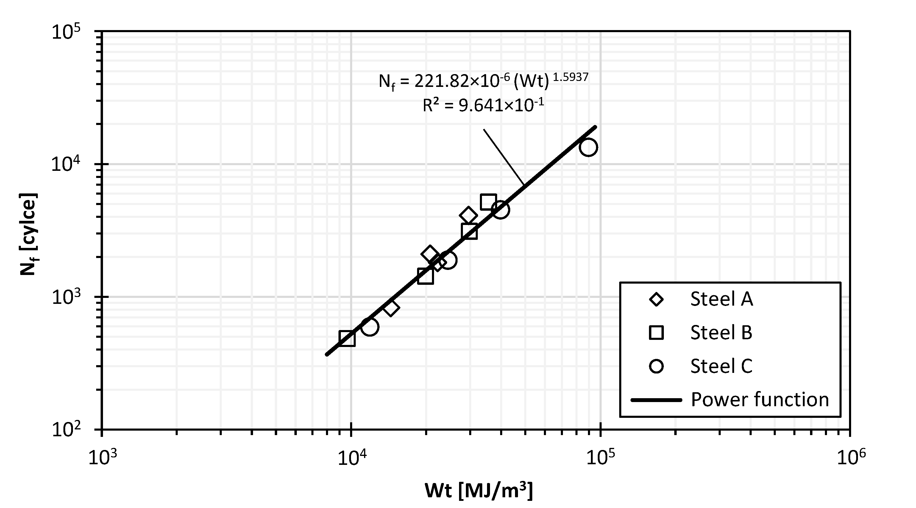
Concerning cumulative total strain energy density, Wt, it was possible to conclude that steel C with higher Mn content disclosed the highest values at strain amplitudes lower than 1.0%, while for ∆
ε/2 = 1.0%, the highest value was exhibited by steel A. In addition, in a log-log scale, there was a direct proportionality between cumulative total strain energy density and the determined fatigue resistance of the tested steels (see
Figure 5). As shown, the data could be successfully fitted by a single power function independent of Mn content and with a high correlation coefficient, which is a major and interesting outcome.
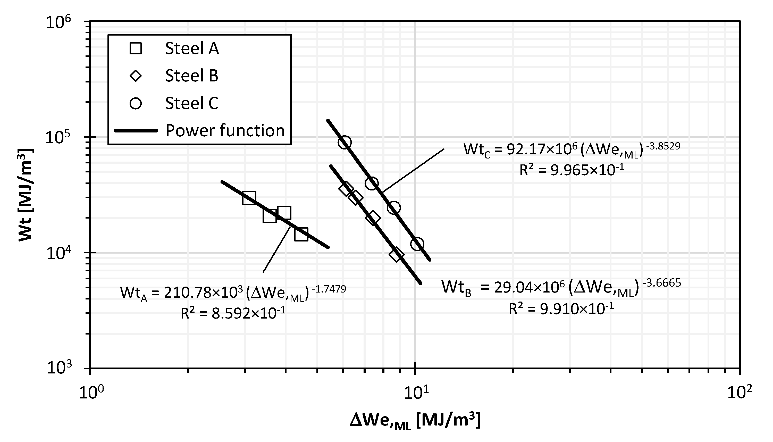
It is also interesting to note that elastic strain energy density of the mid-life cycle (∆
We,
ML) could be correlated with cumulative strain energy density in log-log scales by means of a straight line, as shown in
Figure 6. The values of ∆
We,
ML are summarized in
Table 4. In this case, unlike cumulative total strain energy density versus the number of cycles to failure, the computed curves did not overlap. In the absence of Mn, the curve was shifted to the left. The increase of Mn content moved the curves to the right. Moreover, the slope tended to decrease as the content of Mn rose.
3.2. Fatigue Life Prediction
Numerical fatigue lives were calculated for the three steels under study and the four strain amplitudes applied in strain-controlled fatigue tests using the well-known SWT model (Equation (1)) and the Liu model (Equation (2)). These calculations were performed with the stress and strain values of the mid-life cycle (see
Table 5). After that, numerical results were compared with the obtained experimental data (
Nf) listed in
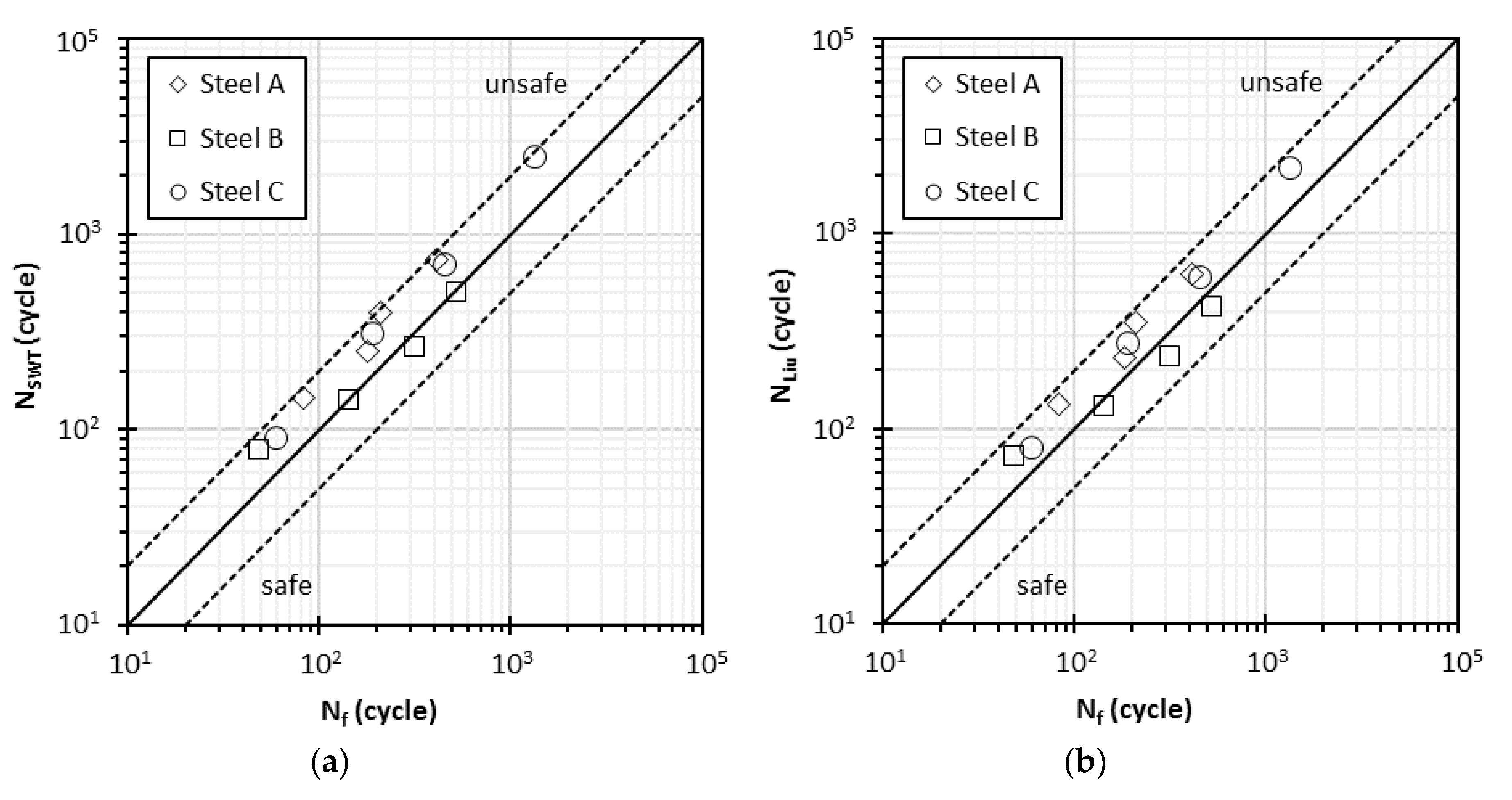
Table 5. For the sake of clarity, a graphical comparison between the predicted and experimental lives is displayed in
Figure 7. As can be seen, numerical predictions were almost exact for steel B and resulted in nonconservative values for steel A and steel C. Furthermore, we could conclude that the Liu criterion led to predictions tendentially safer than the SWT criterion.
Taking into account some inaccuracies of the tested criteria, a new predictive model, based on the cumulative total strain energy density, was developed. The proposed model lies on energy relationships presented in
Section 3.2, more precisely, the power function relating cumulative total strain energy density and the number of cycles to failure (see
Figure 5), and the power functions relating elastic strain energy density of the mid-life cycle and the associated cumulative total strain energy density (see
Figure 6) found for the high-strength bainitic steels under study.
Regarding the determination of elastic strain energy density, defined here as the sum of both the area associated with the linear portion of the descending branch from maximum stress to zero and the area associated with the linear portion of the ascending branch from minimum stress to zero, the calculation could be carried out by means of the following equation:
where ∆
σ is stress range, and
E is Young’s modulus. The stress range for a specific strain amplitude could be estimated from the cyclic curve, i.e.,
where
k′ is the cyclic hardening coefficient and
n′ is the cyclic hardening exponent (see
Table 3). Once the applied stress was known, the associated elastic strain energy density per cycle could be computed from Equation (3). Thus, based on the energy relationships of
Figure 6, we could compute the cumulative total strain energy densities, which allowed the calculation of the corresponding fatigue life from the power function of
Figure 5. The predicted values (N
CTSED) for different strain amplitudes of the three high-strength bainitic steels are presented in
Table 5.
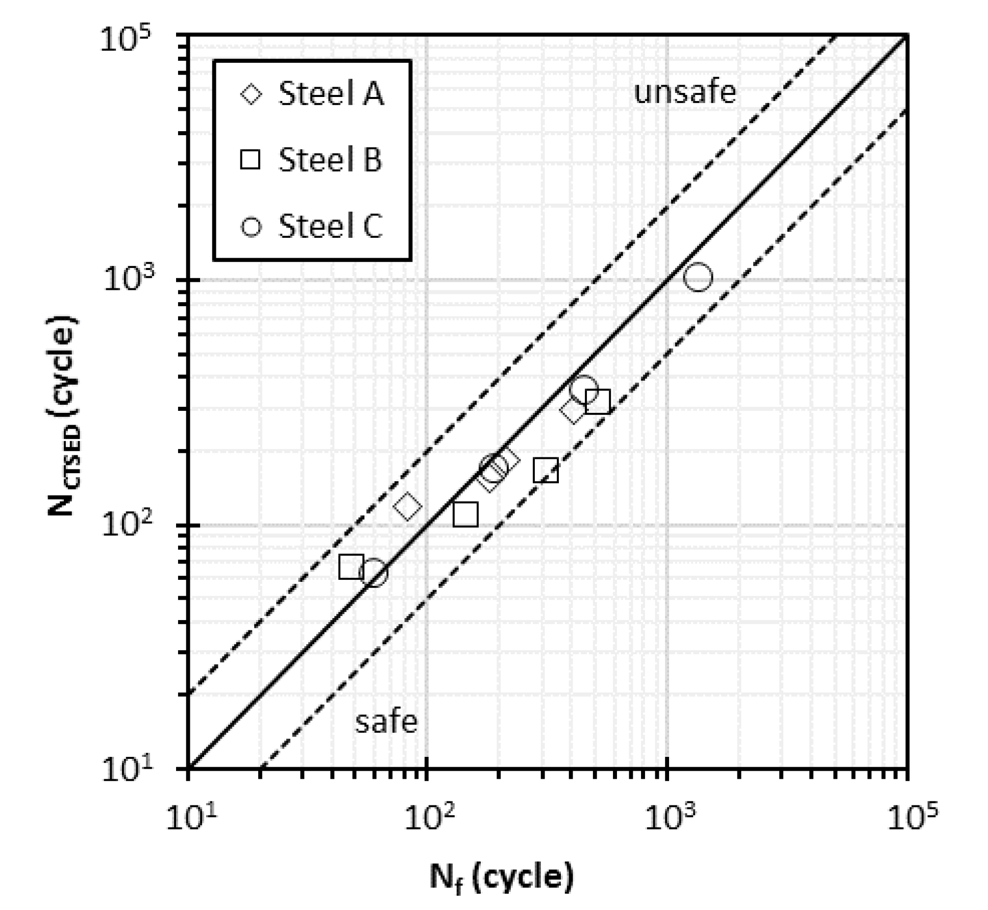
Figure 8 compares the predicted lives with those determined in the experiments. As can be seen, the N
CTSED values were more accurate than those computed through SWT and Liu criteria (see
Figure 7).
In order to analyze the predictive capabilities of the proposed model in a more systematic manner, probability density functions were used, defined from the following error parameter:
where
Np is the predicted lifetime, and
Nf is the experimental life. In theory, more accurate models are those with lower standard deviations and mean errors close to zero. As shown in
Figure 9, the proposed model combined these two features, since it had a mean error closer to zero and a lower standard deviation than the other two. Furthermore, it led to conservative predictions, which was another important outcome.
Table 6 presents several statistical parameters computed from the
Nf/Np ratios obtained for each model, namely minimum error, maximum error, mean, standard deviation and variance. In fact, the cumulative total strain energy density (CTSED) approach led to more accurate results, since its mean deviation was closer to zero and its standard deviation was smaller.


