Hierarchical Path-Planning for Mobile Robots Using a Skeletonization-Informed Rapidly Exploring Random Tree*

Abstract

An efficient, hierarchical, two-dimensional (2D) path-planning method for large complex environments is presented in this paper. For mobile robots moving in 2D environments, conventional path-planning algorithms employ single-layered maps; the proposed approach engages in hierarchical inter- and intra-regional searches. A navigable graph of an environment is constructed using segmented local grid maps and safe junction nodes. An inter-regional path is obtained using the navigable graph and a graph-search algorithm. A skeletonization-informed rapidly exploring random tree* (SIRRT*) efficiently computes converged intra-regional paths for each map segment. The sampling process of the proposed hierarchical path-planning algorithm is locally conducted only in the start and goal regions, whereas the conventional path-planning should process the sampling over the entire environment. The entire path from the start position to the goal position can be achieved more quickly and more robustly using the hierarchical approach than the conventional single-layered method. The performance of the hierarchical path-planning is analyzed using a publicly available benchmark environment.

1. Introduction

Path-planning for mobile robots involves identifying an efficient path from a start position to a goal position on a given environmental map using online sensor data. The path-planning algorithms are divided into those facilitating local and global planning. Local path-planning (“obstacle avoidance”) prevents collisions, even when unexpected (unregistered) obstacles are encountered [1,2]. Global path-planning generates waypoints that connect the start to the goal using the given map [3,4]. In practice, local and global plannings are integrated as the robot proceeds via various waypoints to a goal, while the local planner calculates the actions to arrive at each waypoint using current sensor data. Therefore, the efficient waypoints in safe regions that can constitute the shortest path are essential for higher level applications.

Most global planners initially extract safe/navigable regions from a global map and then find an appropriate path between the safe regions. Safe regions can be represented as empty/unoccupied cells of a grid map or as the nodes of a graph. Grid map-based planning is applicable in two-dimensional (2D) environments because it is possible to directly recognize safe regions and their relationships when planning possible paths between them via regularly decomposed grid cell representation [5,6]. However, to solve scalability issues in high-dimensional applications with limited computational power and time, the grid-based planners require additional effort like the cost approximation [7].

Graph-based methods were developed to handle path-planning in large environments. The computational burdens are lower than those of grid-based methods. The two most widely used approaches are the probabilistic roadmap (PRM) [8] and the rapidly exploring random tree (RRT) [9,10]. These are termed sampling-based methods, because they sample/generate nodes stochastically in empty regions [11,12]. PRM planners first construct a graph (a roadmap) that covers the entire environment and includes collision-free paths. Then, they compute the shortest path from a start position to a goal along the roadmap. Although the multiple-query approach of a PRM planner aids path-planning in complex or high-dimensional spaces [13], many practical path-planning problems can be solved using a single-query approach such as that of an RRT. RRT planners basically expand a tree via random sampling of empty regions from the start position and stop when the tree attains the goal. The RRT variants differ in terms of how they optimize the initial feasible solution or how they modify the tree structure. RRT-Connect simultaneously grows two RRTs rooted at the start and the goal toward each other until they meet, reducing the computational time required for a converged solution [14]. RRT* asymptotically converges to an optimal solution by additionally rewiring the tree [15,16]. RRT*-Connect combines RRT-Connect and RRT*, yielding asymptotically optimal solutions faster than either algorithm alone [17]. Although various RRT algorithms deal with high-dimensional and complex state spaces by ensuring probabilistic completeness and delivering optimal asymptotic solutions, convergence to the optimal solution is slow for environments with narrow passages and when non-solution areas in the entire configuration space are (unnecessarily) subjected to dense sampling [18,19]. The informed RRT* (IRRT*) was developed to improve the convergence rate and the final solution quality by restricting the sampling region to an ellipsoid defined by the solution of the previous optimization step [20]. It obtains a final optimal solution in less time than the basic RRT*. However, as the IRRT* employs a vanilla RRT* sampling method (the sampling target is the entire space) to achieve an initial solution, the IRRT* suffers from problems similar to those of the RRT*.

To overcome the slow convergence rate and reduce the overall processing time by quickly obtaining an initial solution, we previously developed a skeletonization-informed RRT* (SIRRT*) for mobile robots moving in 2D environments [21]. The IRRT* obtains the initial solution using the RRT* algorithm. By contrast, the SIRRT* generates an initial solution by skeletonizing a grid map and constructing a tree on the skeletonized image using Prim’s algorithm [22]. As the convergence rate of the IRRT* algorithm depends on the quality of the initial solution computed by random sampling of the RRT* over the whole space, the IRRT*’s performance is unstable even when the start and goal positions do not change within the same environment. The SIRRT* utilizes the deterministic property of grid map image skeletonization to find the initial solution more robustly and rapidly than the IRRT*. The total computational time required to attain a final solution by the SIRRT* is lower and more repeatable than that required by the IRRT*.

The global path-planning approaches mentioned above assume that an environmental map is available and process the entire map. Thus, path-planning is performed in a single-layer manner. When a part of the map is changed, replanning includes both the unchanged and changed regions. Moreover, we can encounter the situation when the current start and goal positions differ slightly from the start and goal positions of the previously solved problem. The conventional path-planners require sample nodes covering the entire map, although most of the two final solutions may be identical. If we can divide the map and obtain the adjacency between map segments, we can efficiently handle such situations. Sampling-based planners require ever more samples (associated with longer computational times) of larger environments to obtain optimal solutions. If we can construct a environmental graph that contains local path information for each segment and if the graph can be re-used to deal with future path-planning problems, the sampling space can be focused to compute paths more efficiently. Thus inspired, we here propose a hierarchical path-planning method using the SIRRT*.

Earlier global planners have sought to guarantee optimal solutions and reduce computational times; few studies have explored hierarchical path-planning. The focused hierarchical D* (FHD*) is a grid-based, hierarchical, path-planning algorithm seeking to optimize paths by placing bridge nodes on the potential field of the grid map [23]. A three-level hierarchical structure exploiting particle swarm optimization was suggested to yield feasible, safe, and optimal paths [24]. However, its hierarchy means the algorithmic structure is composed of map decomposition and path optimization; the method does not reveal the hierarchical geometric structure of the environment. A hierarchical roadmap (HRM), similar to what we develop here, can be incrementally constructed via normalized graph-cut segmentation of a local sonar grid map [25].

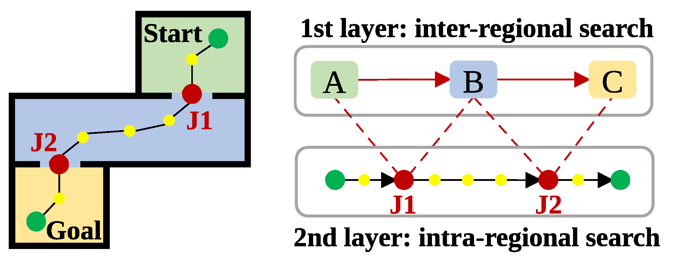
Here, a two-layered, hierarchical path-planning method is developed. The combined method of the previous work, the SIRRT*, and the well-known image segmentation method, the watershed segmentation, is presented. A global path, thus a sequence of path regions from a start region to a goal region, is firstly obtained through the segmented grid map. Within each path region, the SIRRT* is applied to compute a local path between two junction nodes. An entire path from the start to the goal is generated by combining these local paths. Figure 1 illustrates the proposed hierarchical path-planning method. The local grid maps (A, B, and C) and the junction nodes (J1, J2) between adjacent local maps constitute a graph. The local paths within local grid maps, defined via intra-regional searching, are combined using the inter-regional path. The proposed approach can be applied to most mobile robots operated in 2D environments, including wheeled mobile robots and legged mobile robots. The proposed hierarchical planning is a kind of divide-and-conquer method, and it suggests the required sequence and its corresponding components from environmental segmentation to database construction. The contribution of this paper lies in the overall sequence for hierarchical path-planning. Although divide-and-conquer or local-metric/global-topological approaches have already been discussed in other research areas, we need to consider additional components to apply them to practical path-planning problems. Especially, a navigable graph structure, which is a database of local paths, is constructed by the SIRRT*. The previous works, for SIRRT* planning, show robust performance for multiple running applications, and it is efficient for constructing the navigable graph structure.

The remainder of the paper is organized as follows. In Section 2, a navigable graph of an environment is constructed; we segment the grid map and extract junction nodes between two adjacent segments. In Section 3, the hierarchical path-planning algorithm using the navigable graph is developed; we employ the Dijkstra graph-search for inter-regional path-planning and the SIRRT* intra-regional path-planning to this end. Section 4 describes the experimental results using a well-known (benchmark) environment to verify the efficacy of the proposed hierarchical approach. Section 5 contains conclusions and future directions.

2. Navigable Graph of an Environment

This section shows how to construct a navigable graph of an environment. The grid map image is firstly segmented using a watershed segmentation algorithm. Then, junction nodes lying on edge grid cells separating adjacent segments are defined.

2.1. Grid Map Segmentation

Many studies have explored environmental segmentation, and most have sought to construct topological maps by extracting the nodes and edges of empty areas defined using various metrics by reference to a generalized Voronoi graph (GVG) [26,27,28]. Using the positions of nodes, the environment can be easily segmented so that each grid cell is assigned to the nearest node; cells assigned to the same node are in the same segment. Other studies have focused more on dividing a grid map [29]. RoomSegis a watershed, grid map segmentation method used to guide autonomous cleaning robots in large environments and is a practical end-to-end implementation even if the grid map is noisy [30]. It is possible to divide a consecutive, local sonar grid map into two regions via cell decomposition and the normalized graph cut method and incrementally segment the environment to construct a connected graph [31,32].

A watershed algorithm that is easily implemented and that yields reliable segmentation results is applied to the grid map segmentation in this paper. We engage in hierarchical path-planning using a navigable graph of segmented local grid maps; we do not engage in grid map segmentation per se. The watershed transform detects catchment basins in a grayscale image by considering the image as a topographic relief; the height of each pixel is proportional to its gray level [33]. As the grid map is considered a black (occupied)-and-white (empty) binary image, it must be converted to impart various intensities to empty cells. A distance transform operator is used to calculate the distance to the closest boundary (an occupied cell) from each empty cell. 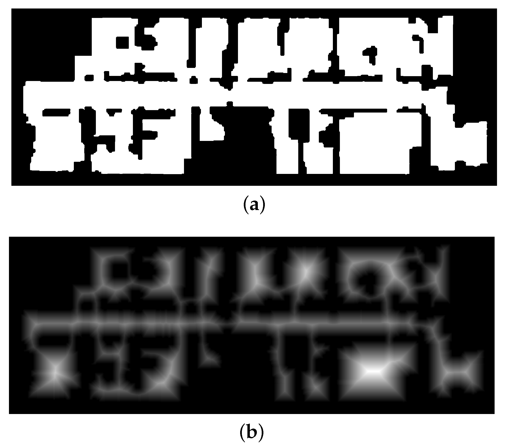Figure 2a shows a grid map image of a public benchmark environment [34], and the grid map image is obtained by constructing a grid map using laser measurements and converting it to a binary image. Figure 2b shows the normalized distance transform image computed using the Euclidean distance metric.

Use of the basic watershed segmentation algorithm can cause over-segmentation. Figure 2c shows the segmentation result of the distance transform image of Figure 2b, computed using the basic watershed algorithm. To overcome this problem, a marker-controlled, watershed segmentation algorithm has been developed [33,35]. This uses markers to indicate initial segment information, thus the number and approximate positions of objects or foregrounds that can be definitely distinguished from backgrounds. Markers are computed using morphological operations such as erosion and dilation. Prior to the watershed application to the grid map, the definite background pixels (occupied cells) are easily recognized from the grid map image; this is not the case for other gray-scale images. When path-planning, we are interested in safe navigable areas (empty cells) and calculate the distance transforms for all such cells. The pixels lying further from occupied cells are considered as definitive foreground segments. The empty cells that exceed the threshold value of the normalized distance transform serve as marker regions. Markers are labeled using the connected components labeling (CCL) algorithm (which assigns unique labels to all pixels in each connected segment). Figure 2d shows the labeled markers; these are combined with the empty cell information of Figure 2e. The marker-controlled watershed algorithm gradually grows regions and decides the segment to which each non-labeled empty cell belongs. Marker-controlled segmentation is shown in Figure 3a.

2.2. Junction Node Extraction

The watershed segmentation algorithm produces several grid map segments with different labels, separated by edges/boundaries one pixel in width. To construct a navigable graph using the segments, the junction nodes between adjacent segments must be defined. In the proposed path-planning method, these nodes serve as sub-goals/waypoints, allowing movement to the next path regions, defined as local regions through which the robot must pass.

Algorithm 1 shows how to extract junction nodes, $Node$, and how to construct the adjacency matrix, $Adj$, of the grid map segments. Algorithm 1 requires two inputs, $gridma{p}_{\mathrm{dist}}$ and $gridma{p}_{\mathrm{WS}}$. $gridma{p}_{\mathrm{dist}}$ is the normalized distance transform of the grid map, and $gridma{p}_{\mathrm{WS}}$ is the watershed segmentation result where each pixel value shows the label identification of the corresponding segment. The algorithm first inspects all edges of cells, $gri{d}_{\mathrm{edge}}$, in the watershed segmentation result and combines the edge cells that share neighbors into a matricized form, $Ad{j}^{\mathrm{cells}}$, wherein each component is a group of cells lying between the same adjacent segments (Lines 4–10). $Adj$ is the adjacency matrix among grid map segments. If there are M segments, the size of the symmetric matrix $Adj$ is M. If there are any edge cells between two segments i and j, $ad{j}_{i,j}$ and $ad{j}_{j,i}$ are one (Line 8). Each component $ad{j}_{i,j}^{\mathrm{cells}}$ of $Ad{j}^{\mathrm{cells}}$ stores all edge cells between two segments i and j (Line 7).

For each group of edge cells, we inspect and obtain the connected edge segments using the CCL (Line 13), which can deal with the situation in which two adjacent grid map segments can be connected via several separate edge areas. The junction node should be the safest grid cell; thus, we select the cell exhibiting the maximum, normalized distance transform value with respect to one of the connected edge segments (Line 16). Finally, we obtain the junction nodes and the adjacency matrix of the grid map segments (Line 20).

Algorithm 1 Junction node extraction.

Require:$gridma{p}_{\mathrm{dist}},gridma{p}_{\mathrm{ws}}$ Ensure: junction nodes $Node=\left\{nod{e}_{i,j}^n|1\le n\le N,N\mathrm{is}\mathrm{the}\mathrm{number}\mathrm{of}\mathrm{junction}\mathrm{nodes}.\right\}$, adjacency matrix among grid map segments $Adj$   1:  function Select-Junction-Node($gridma{p}_{\mathrm{dist}},gridma{p}_{\mathrm{ws}}$)   2:     Set $Ad{j}^{\mathrm{cells}}=\left\{ad{j}_{i,j}^{\mathrm{cells}}|ad{j}_{i,j}^{\mathrm{cells}}=\varnothing ,1\le i,j\le M,M\mathrm{is}\mathrm{the}\mathrm{number}\mathrm{of}\mathrm{segments}.\right\}$   3:     Set $Adj=\left\{ad{j}_{i,j}|\mathrm{the}\mathrm{identity}\mathrm{matrix}\mathrm{of}\mathrm{size}M\times M,M\mathrm{is}\mathrm{the}\mathrm{number}\mathrm{of}\mathrm{segments}.\right\}$     ▹ Grouping edge cells that have the two same neighboring segments and calculating the adjacency   4:     for all $gri{d}_{\mathrm{edge}}\in gridma{p}_{\mathrm{ws}}$ do   5:         Inspect eight neighbor cells around $gri{d}_{\mathrm{edge}}$.   6:         if there are two different labeled neighbors, and their labels are i and j then   7:            $ad{j}_{i,j}^{\mathrm{cells}}\leftarrow ad{j}_{i,j}^{\mathrm{cells}}\cup \left\{gri{d}_{\mathrm{edge}}\right\},ad{j}_{j,i}^{\mathrm{cells}}\leftarrow ad{j}_{i,j}^{\mathrm{cells}}$   8:            $ad{j}_{i,j}\leftarrow 1,ad{j}_{j,i}\leftarrow ad{j}_{i,j}$   9:         end if   10:     end for   11:     $n\leftarrow 0$     ▹ Selecting junction node cells for each group of edge cells in $Ad{j}^{cells}$   12:     for all non-empty $ad{j}_{i,j}^{\mathrm{cells}}\in Ad{j}^{cells}$ do     ▹$ad{j}_{i,j}^{\mathrm{cells},1}\cup \cdots \cup ad{j}_{i,j}^{\mathrm{cells},K}=ad{j}_{i,j}^{\mathrm{cells}}$, K is the number of disconnected edge segments in $ad{j}_{i,j}^{\mathrm{cells}}$.   13:         $\left\{ad{j}_{i,j}^{\mathrm{cells},1},\cdots ,ad{j}_{i,j}^{\mathrm{cells},K}\right\}\leftarrow \mathrm{connected}\_\mathrm{component}\_\mathrm{labeling}\left(ad{j}_{i,j}^{\mathrm{cells}}\right)$   14:         for all $ad{j}_{i,j}^{\mathrm{cells},k}$ do   15:            $n\leftarrow n+1$            ▹ The safest cell with the maximum distance to obstacles is selected as a junction node.   16:            Select one cell $gri{d}_{d_{\max }}$ in $ad{j}_{i,j}^{\mathrm{cells},k}$ with the maximum $gridma{p}_{\mathrm{dist}}$.   17:            $nod{e}_{i,j}^n\leftarrow gri{d}_{d_{\max }}$   18:         end for   19:     end for   20:     return $Node,Adj$   21: end function

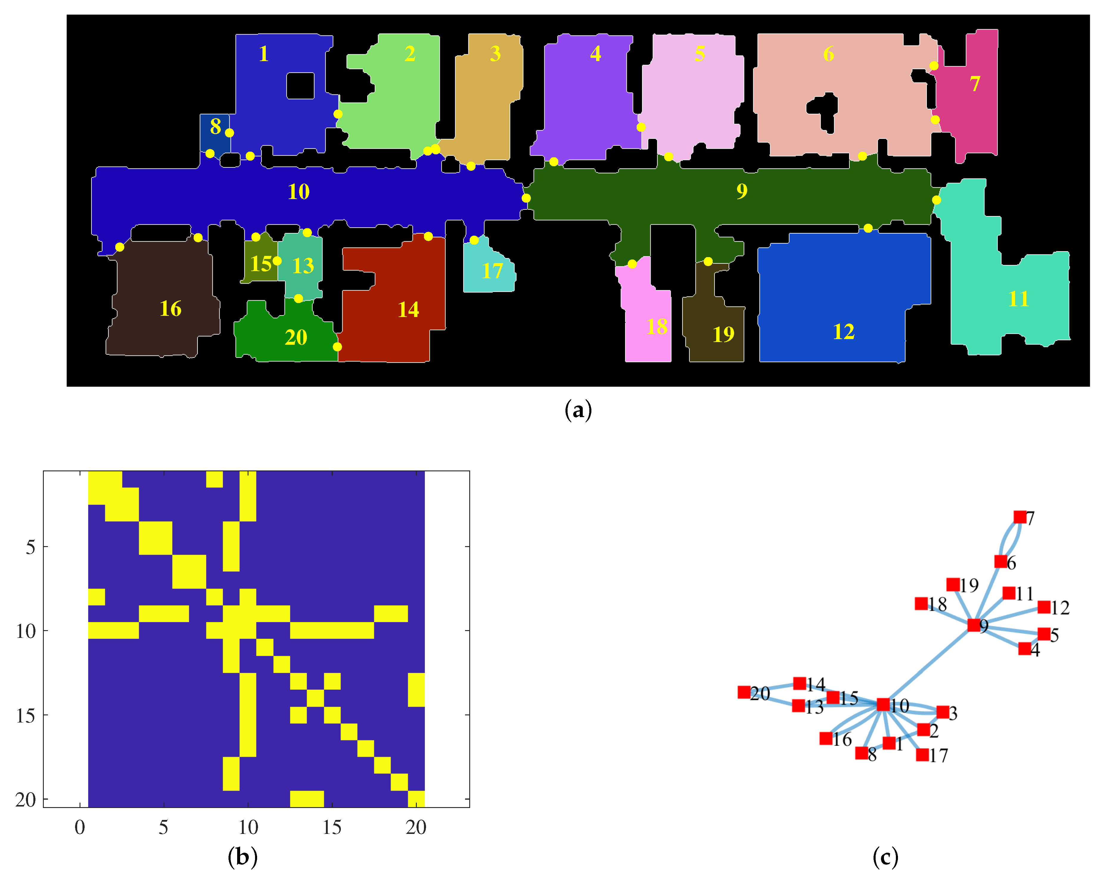
Figure 3 shows the graph structure of the segmented grid map. In Figure 3a, the yellow dots are the junction nodes, and the numbers identify the segments. Figure 3b is the corresponding adjacency matrix. In Figure 3a, Segments “6” and “7” are structurally connected in two separate places. Two segments in Figure 3c feature two edges and two junction nodes.

3. Hierarchical Path-Planning

In this section, the hierarchical path-planning method using the graph-search algorithm and the SIRRT* is developed. Previously, a navigable graph of the environment consisting of local grid map segments, the adjacency matrix, and the junction nodes between all adjacent segments was constructed. We now use the SIRRT* to compute intra-regional paths among the junction nodes of each grid map segment. Figure 4 shows the SIRRT* result for Segment “9”. The initial solution path is computed using the Harris corner nodes of the skeletonized grid map image and Prim’s algorithm (Figure 4a–c). The final path is obtained via informed sampling optimization (Figure 4d).

Figure 5 shows the overall procedure of the proposed method. The first layer in path-planning is an inter-regional search using the navigable graph structure of the segmented grid maps; we find a start region and a goal region (A). Then, the inter-regional path from the start region to the goal region is computed using the adjacency matrix and the graph-search algorithm (B). The Dijkstra graph-search algorithm is employed to this end; all adjacent segment pairs are equally weighted during the inter-regional search. When the inter-regional path is defined, the junction nodes are selected (C) to yield the SIRRT* paths among those nodes for each path region. At this time, several junction nodes for two adjacent segments can be selected because obstacles may lie between the segments. Thus, two adjacent segments can be connected at several nodes. To ensure that the junction node sequence from the start to the goal is efficient, we construct a cost matrix. The SIRRT* yields the intra-regional paths from the start to the junction nodes of the start region and from the goal to the junction nodes of the goal region (D). The cost matrix is calculated by the costs of the SIRRT* paths (E). By using the cost matrix and the Dijkstra graph-search algorithm, the node sequence from the start position to the goal position can be computed (F). The graph-search algorithm selects the cheapest junction nodes. Finally, a global path is achieved by combining the intra-regional paths with reference to the node sequence (G).

Algorithm 2 is the pseudocode of the hierarchical path-planning, and it describes the procedure after obtaining the inter-regional path from the start region, $se{g}_S$, to the goal region, $se{g}_G$. $Seg$ is the sequence of the path regions according to the inter-regional path, and K is the number of the path regions. Algorithm 2 also requires the navigable graph structure including the junction nodes, $Nod{e}_{JC}$, and the intra-regional paths, $Path$, of all segments. The junction nodes, $Nod{e}_{\mathrm{path}}$, are selected according to the inter-regional path, $Seg$, in Lines 2–5. The intra-regional paths, $Pat{h}_S$, from the start position to the junction nodes of the start region are computed by the SIRRT* (Lines 6–10). The intra-regional paths, $Pat{h}_G$, from the goal position to the junction nodes of the goal region are also computed by the SIRRT* (Lines 11–15). The cost matrix, $Cos{t}_{JC}$, among the selected junction nodes, the start position, and the goal position is obtained in Lines 16–26. If M is the number of the selected junction nodes, $Nod{e}_{path}$, the size of the symmetric cost matrix is $M+2$. The cost values between the start/goal to the selected junction nodes should be added to the cost matrix. Using the cost matrix, the Dijkstra graph-search algorithm computes the node sequence, $Nod{e}_{SG}$, from the start to the goal. Here, the indices of the start and the goal in the cost matrix are $M+1$ and $M+2$, respectively (Line 27). By connecting the intra-regional paths in series, we obtain the final path, $Pat{h}_{SG}$ (Line 28).

Figure 6a,c,e shows the hierarchical path-planning results derived using three different starts and goals, and Figure 6b,d,f is the corresponding cost matrices for the selected junction nodes along the inter-regional paths. As shown in Figure 6a, the inter-regional path is $16\to 10\to 9\to 6\to 7$. The cyan squares are the selected junction nodes, or $Nod{e}_{\mathrm{path}}$ of the path regions in Algorithm 2. As Segment “7” is connected to Segment “6” through two junction nodes, both nodes were selected when computing the cost matrix. The second-to-last entries of the cost matrix are the SIRRT* distances from the start to the junction nodes of the start region and the last entries the SIRRT* distances from the goal to the junction nodes of the goal region. Such path-planning chooses the most efficient junction nodes when computing a global path using the cost matrix and the graph-search algorithm.

Algorithm 2 Hierarchical path-planning.

Require: the inter-regional path from the start region, $se{g}_S$, to the goal region, $se{g}_G$, $Seg=\left\{se{g}_k|1\le k\le K,se{g}_1=se{g}_S,se{g}_K=se{g}_G\right\}$, junction nodes $Nod{e}_{JC}=\left\{nod{e}_{i,j}^n|1\le n\le N\right\}$, where N is the number of junction nodes, $nod{e}_{i,j}^n$ is the junction node between $se{g}_i$ and $se{g}_j$, and the SIRRT* paths among the junction nodes $Path=\left\{pat{h}_{p,q}^{se{g}_i}|p,q\in Nod{e}_{JC},se{g}_i\in Seg\right\}$ Ensure: the final path $Pat{h}_{SG}$ that is a sequence of waypoints from the start to goal positions   1: functionHierarchical SIRRT*($Seg$, $Nod{e}_{JC}$, $Path$)   2:     Set $Nod{e}_{\mathrm{path}}=\varnothing$     ▹ Selecting the junction nodes ($Nod{e}_{\mathrm{path}}$) according to the inter-regional path   3:     for $se{g}_k\in Seg,1\le k\le K-1$ do   4:         Find all $nod{e}_{k,k+1}^n\in Nod{e}_{JC}$. $Nod{e}_{\mathrm{path}}\leftarrow Nod{e}_{\mathrm{path}}\cup \left\{nod{e}_{k,k+1}^n\right\}$   5:     end for     ▹ Computing the intra-regional path ($Pat{h}_S$) from the start position to the junction nodes   6:     Set $Pat{h}_S=\varnothing$.   7:     for all $nod{e}_{1,k}^n\in Nod{e}_{\mathrm{path}}$ do   8:         Compute the SIRRT* path $pat{h}_{S,n}^{se{g}_1}$ from the start position to $nod{e}_{1,k}^n$ of $se{g}_1=se{g}_S$.   9:         $Pat{h}_S\leftarrow Pat{h}_S\cup \left\{pat{h}_{S,n}^{se{g}_1}\right\}$                       ▹$n\in Nod{e}_{\mathrm{path}}$   10:     end for     ▹ Computing the intra-regional path ($Pat{h}_G$) from the goal position to the junction nodes   11:     Set $Pat{h}_G=\varnothing$.   12:     for all $nod{e}_{k,K}^n\in Nod{e}_{\mathrm{path}}$ do   13:         Compute SIRRT* path $pat{h}_{n,G}^{se{g}_K}$ from the goal position to $nod{e}_{k,K}^n$ of $se{g}_K=se{g}_G$.   14:         $Pat{h}_G\leftarrow Pat{h}_G\cup \left\{pat{h}_{n,G}^{se{g}_K}\right\}$                      ▹$n\in Nod{e}_{\mathrm{path}}$   15:     end for     ▹ Calculating the cost matrix among the selected junction nodes and start/goal positions   16:     Set a zero-matrix $Cos{t}_{JC}=\left\{cos{t}_{i,j}|1\le i,j\le M+2\right\}$   17:     for $se{g}_k\in Seg,2\le k\le K-1$ do   18:         Find all pairs of $nod{e}_{k-1,k}^i$, $nod{e}_{k,k+1}^j$ ∈$Nod{e}_{path}$.          ▹$Nod{e}_{path}\subset Nod{e}_{JC}$   19:         $cos{t}_{i,j}$ and $cos{t}_{j,i}$← the cost of $pat{h}_{i,j}^{se{g}_k}\in Path$   20:     end for   21:     for all $pat{h}_{S,n}^{se{g}_1}\in Pat{h}_S$ do   22:         $cos{t}_{n,M+1}$ and $cos{t}_{M+1,n}$← the cost of $pat{h}_{S,n}^{se{g}_1}$   23:     end for   24:     for all $pat{h}_{n,G}^{se{g}_K}\in Pat{h}_G$ do   25:         $cos{t}_{n,M+2}$ and $cos{t}_{M+2,n}$← the cost of $pat{h}_{n,G}^{se{g}_K}$   26:     end for   27:     A node sequence $nod{e}_S$ to $nod{e}_G$, $Nod{e}_{SG}$← Dijkstra_Graph_Search($Cos{t}_{JC}$, $M+1$, $M+2$)   28:     Obtain the final path, $Pat{h}_{SG}$, by combining the intra-regional paths according to $Nod{e}_{SG}$.   29:     return $Pat{h}_{SG}$   30: end function

4. Experimental Results

The proposed hierarchical path-planning method was analyzed to verify its stable and efficient performance. All experiments were performed on an Intel Core i7-9700K (eight cores of 3.6 GHz) with 32 GB of memory in the same benchmark environment; several rooms were connected by corridors, as in the real world.

The SIRRT* was compared with the IRRT* to verify that the SIRRT* is more efficient in constructing the proposed navigable graph structure that needs multiple intra-regional planning runs among junction nodes. The stability of the SIRRT* in terms of computational time and the final costs is shown in

Table 1. A comparison of the IRRT* and the SIRRT*.

		# of Iterations for Optimization
		1000		2000		3000
		IRRT*	SIRRT*	IRRT*	SIRRT*	IRRT*	SIRRT*
Computational time (s)	Mean	8.01	0.51	8.74	0.83	7.46	1.19
	Std.	5.86	0.08	6.59	0.11	7.39	0.12
	Min.	1.02	0.37	1.45	0.59	1.23	0.93
	Max.	32.08	0.72	40.08	1.14	49.04	1.44
Final cost (pixels)	Mean	1441.27	1555.33	1451.28	1535.60	1442.94	1516.71
	Std.	61.90	16.53	64.49	21.65	54.54	20.52
	Min.	1389.36	1506.31	1388.81	1475.96	1390.23	1465.13
	Max.	1680.39	1583.75	1676.32	1577.36	1630.01	1563.89
# of total iterations	Mean	7611.26		7469.60		7106.37
	Std.	2684.09		2353.94		2895.54
	Min.	3758.00		3610.00		3669.00
	Max.	16,027.00		15,124.00		20,554.00

. The start and goal positions are given in Figure 6a. The IRRT* and SIRRT* performed 1000, 2000, and 3000 informed sampling optimizations after obtaining an initial solution. For each optimization number, one-hundred experiments were performed. In the SIRRT*, the initial solution is deterministically computed by skeletonization employing the Harris corner detector; random sampling is not in play. However, the IRRT* algorithm uses RRT* sampling to achieve an initial solution throughout the entire environment. The total number of IRRT* iterations is the sum of the RRT* samplings required until an initial solution is obtained and the number of informed samplings required for optimization.

As the IRRT* performs the RRT* sampling to obtain an initial solution, the computational time is negatively affected. If initial solution computation is slow, the number of RRT* samplings increases, as does the computational time. The mean IRRT* computational times were 8.01, 8.74, and 7.46 s. However, the differences were not significant; the SDs were very large (5.86, 6.59, and 7.39 s). Thus, the IRRT* performed very differently during each trial, although the start and goal positions were the same. By contrast, the SIRRT* computational times were faster and more stable (means 0.51, 0.83, and 1.19 s) than those of the IRRT*. The SDs were relatively small at 0.08, 0.11, and 0.12 s. The SIRRT* generated initial solutions faster than did the IRRT*, and the total computational time for the final solution was lower and more robust than that of the IRRT*. The final costs of the SIRRT* were relatively larger than those of the IRRT*. However, the IRRT* SDs were larger than those of the SIRRT*. Sampling-based algorithms such as the RRT variants are more likely to achieve an optimal solution as the number of samples increases. The larger number of the total IRRT* iterations reduced the mean final cost, but at the expense of large SDs. Constructing the navigable graph structure requires conducting the local planning algorithm multiple times to obtain the intra-regional paths among junction nodes. Therefore, the SIRRT* that shows more consistent results (low SDs) is efficient for the hierarchical planning approach.

The hierarchical path-planning method consists of two phases: we construct a navigable graph of the environment featuring grid map segmentation and the SIRRT*-mediated path computation among the junction nodes of each segment, then we engage in inter- and intra-regional path-planning using the graph.

Table 2. Computational times (s) for constructing a navigable graph structure when the numbers of path optimization iterations varied.

# of Iterations for Optimization
1000			2000			3000
Mean (Std.)	Min.	Max.	Mean (Std.)	Min.	Max.	Mean (Std.)	Min.	Max.
44.33 (0.90)	42.70	45.78	108.13 (1.89)	104.82	111.36	196.05 (4.48)	189.12	202.16

shows the computational times required for the construction of navigable environmental graphs using different numbers of the SIRRT* optimization iterations. The number of such iterations is the number of ellipsoidal-informed samplings performed after obtaining an initial solution via skeletonization. For each fixed iteration number of the SIRRT* optimization, thirty experiments were performed. The environment was divided into 20 local segments, and twenty-eight junction nodes were registered. As all intra-regional paths were defined using the SIRRT*, the SIRRT* algorithm totally ran 117 times for each experiment. Therefore, the computational times in Table 2 reflect 117 SIRRT* path-plannings. The SIRRT* algorithm exploits the deterministic feature of skeletonization and the random nature of the RRT*, thus affording more stable performance than the other RRT* variants. Even after many trials, the standard deviations (SDs) were small; it is appropriate to construct the navigable graph via multiple computations of local paths in each grid map segment.

Table 3. Hierarchical path-planning using the pre-built map; 3000 iterations.

		# of Iterations for Optimization
		50	100	200	500	1000	2000	3000
Computational time (s)	Mean	0.28	0.36	0.56	1.49	3.93	11.20	21.94
	Std.	0.02	0.02	0.03	0.06	0.07	0.14	0.28
	Min.	0.25	0.32	0.52	1.40	3.83	11.06	21.51
	Max.	0.32	0.40	0.63	1.63	4.07	11.57	21.51
Final cost (pixels)	Mean	1420.60	1420.00	1420.00	1420.00	1420.00	1420.00	1420.00
	Std.	2.18	0.00	0.00	0.00	0.00	0.00	0.00
	Min.	1420.00	1420.00	1420.00	1420.00	1420.00	1420.00	1420.00
	Max.	1431.00	1420.00	1420.00	1420.00	1420.00	1420.00	1420.00

shows the hierarchical path-planning results including the inter- and intra-regional path-planning. The starts and goals are those of Table 1. The pre-constructed navigable graph featured 3000 SIRRT* iterations; we performed 100 runs for each iteration number of the SIRRT* optimization. The iteration number of the SIRRT* optimization reveals intra-regional paths from the start and goal positions to the junction nodes. Computationally, global path calculation time increased as the number of iterations increased. When sampling-based planners were used, the time required and the sample number increased as the search area increased. In the experiments of Table 1, we searched the entire environment; optimization required many samples. However, hierarchical intra-regional searches of start and goal positions were performed on environmental segments. Intra-regional searches do not require large numbers of samples. After only 100 iterations, the converged final path was apparent. Cost was reduced if the navigable graph featured over 3000 iterations. Moreover, the proposed hierarchical planning based on the SIRRT* yielded smaller SDs.

Figure 7 shows the comparison of the IRRT*, the SIRRT*, and hierarchical path-planning (the H-SIRRT*). Each graph component presents the mean, minimum, and maximum values for 100 runs. As mentioned earlier, because the results of the IRRT* have large differences for each run, it cannot be suitable for practical real-time applications. Moreover, even with the low number of optimization iterations after obtaining the initial solution, the IRRT* required too many iterations to achieve the initial solution, making the total computational time high. As shown in Figure 6a, the start region and the goal region have two junction nodes. The hierarchical path-planning includes the inter-regional graph-search and four intra-regional path-plannings using the SIRRT*. Therefore, the computational time of the hierarchical planning is higher than that of the SIRRT*. The sampling areas of the hierarchical planning’s intra-regional planning are restricted as the small parts of the entire environment. In contrast, the sampling area of the SIRRT* is the whole environment. The hierarchical planning can achieve the lower cost solution using only a lower number of optimization iterations.

5. Conclusions

A hierarchical path-planning method using a navigable graph structure of the environment evaluated via the SIRRT* was proposed in this paper. Conventional global path-planning algorithms find optimal paths by processing entire single-layer environments. In the proposed approach, paths are identified on the intrinsic hierarchical structure; inter- and intra-regional searches are performed. The navigable, environmental graph structure using local map segments and safe junction nodes is defined in the hierarchical path-planning. The inter-regional paths from start regions to goal regions are revealed when navigable graph structures are explored using the Dijkstra graph-search algorithm; the intra-regional paths are computed using the SIRRT*. The hierarchical approach assured stable and efficient performance. The SIRRT* was compared with the IRRT*; the SIRRT* was optimal for the proposed hierarchical path-planning because the SDs of the computational times were lower than those of the IRRT*. Experimentally, hierarchical path-planning using the SIRRT* (over various iterations) afforded efficient, final path convergences (from the start to the end) using few iterations. The proposed method will aid stable and efficient path-planning in large environments.

The proposed method assumes a general global planning situation when a robot finds a global path from the start to the goal before it starts to navigate. Although we can use local planners in dynamic environments, global planners also need to cope with dynamic situations in real time. The hierarchical approach can efficiently handle such dynamic situations because it can re-plan the path by performing the intra-regional planning in the changed area and connecting the new intra-regional path with the inter-regional path. Detecting dynamic obstacles and integrating them into the navigation framework in highly dynamic environments need to be investigated in the future. In addition, applying the proposed approach to non-grid-based maps can be valuable for a wide range of practical applications.