Dynamics Modelling and Simulation for Deployment Characteristics of Mesh Reflector Antennas


Abstract
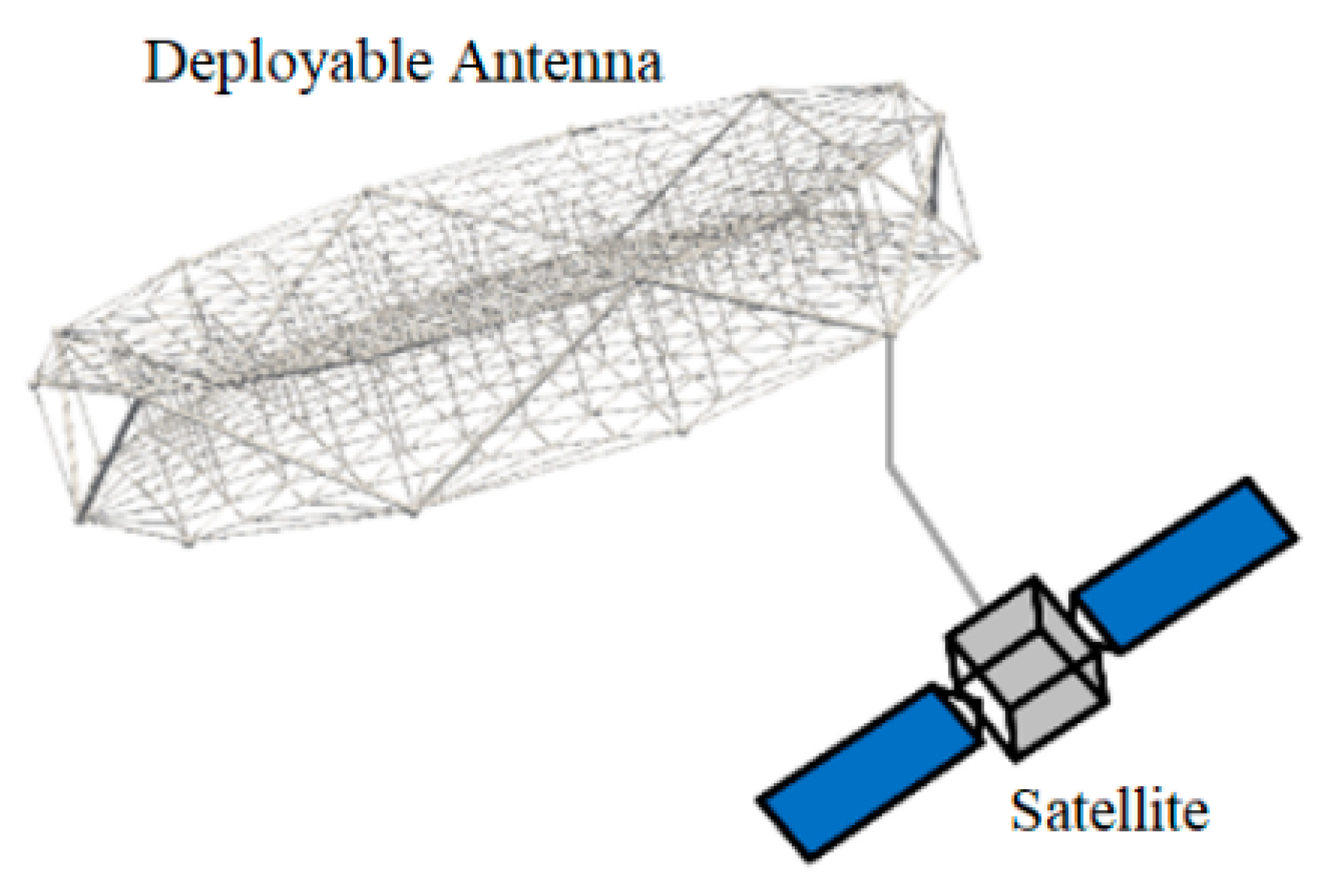
:1. Introduction
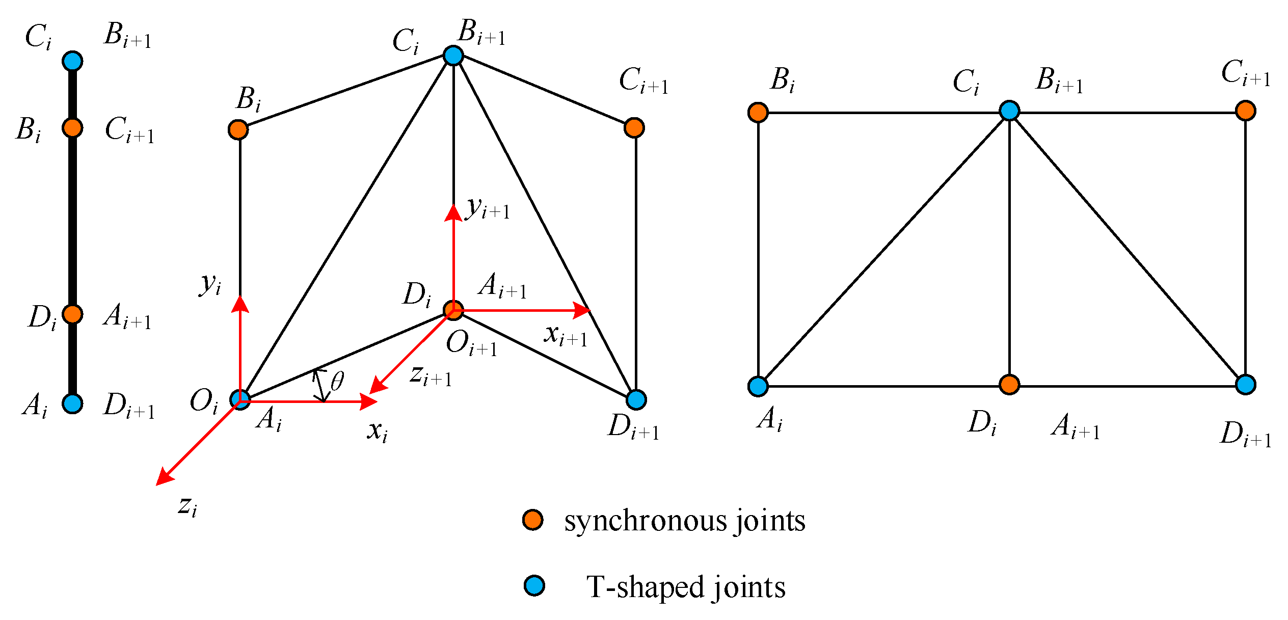
2. Dynamic Modelling of the Truss Antenna
2.1. Dynamic Equations of Truss
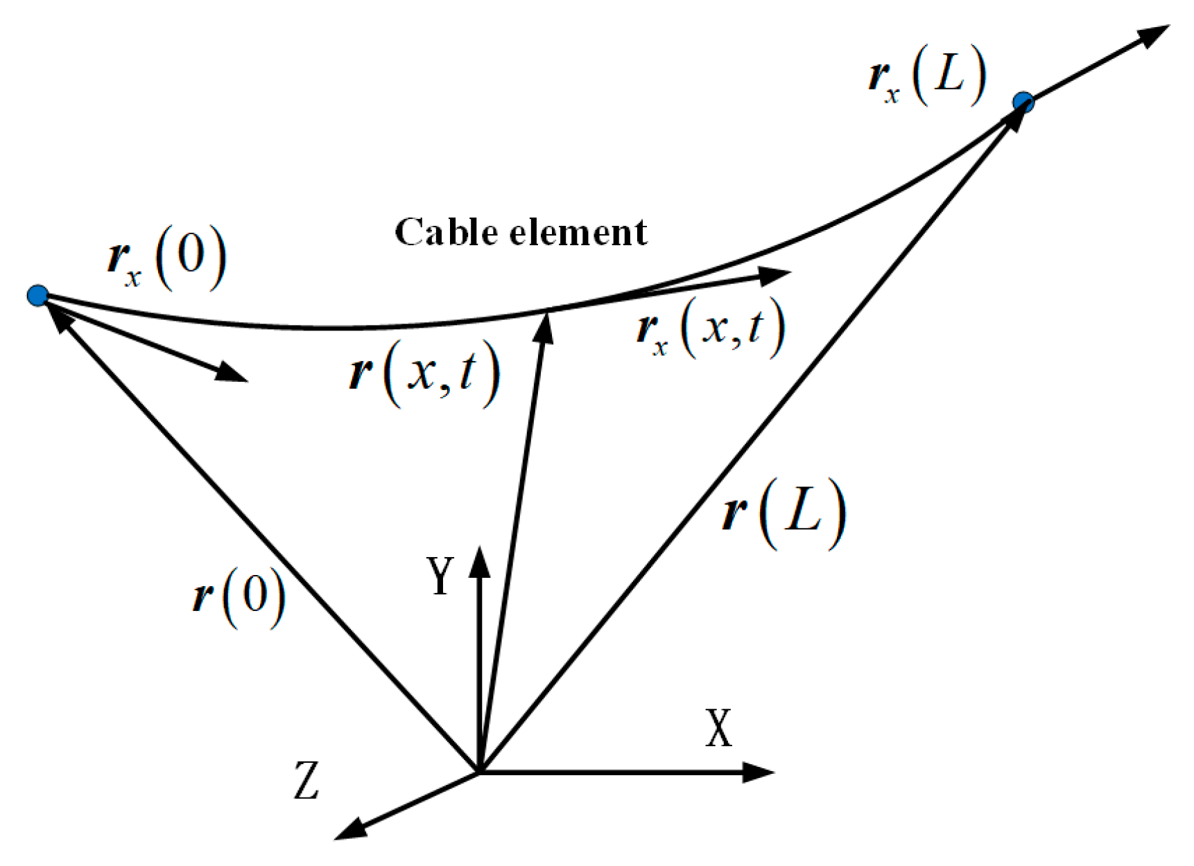
2.2. Dynamic Equations of Cable Net
2.3. Dynamic Equations of System
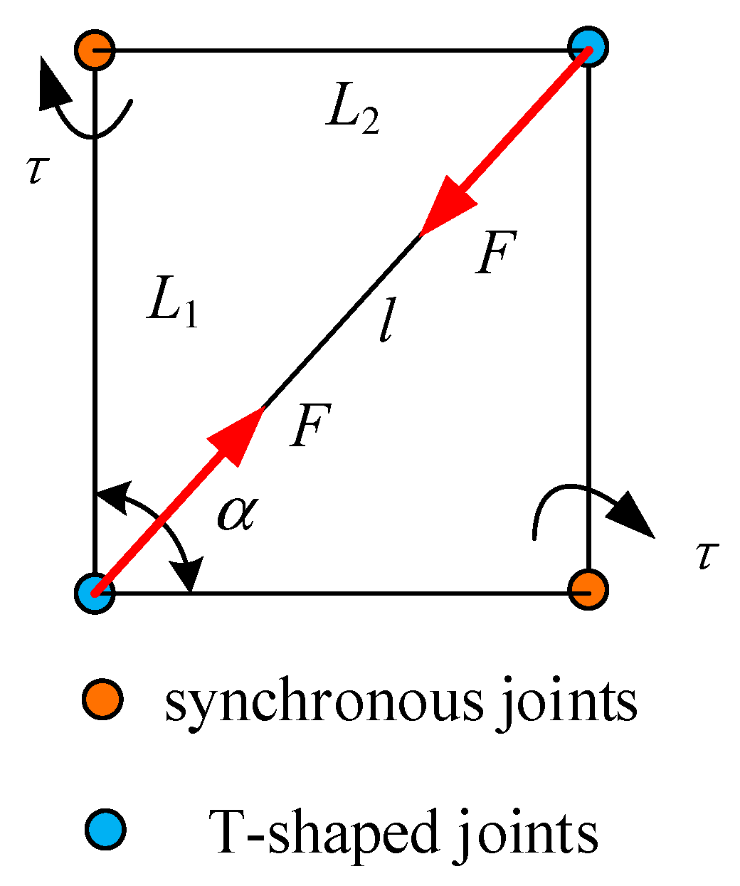
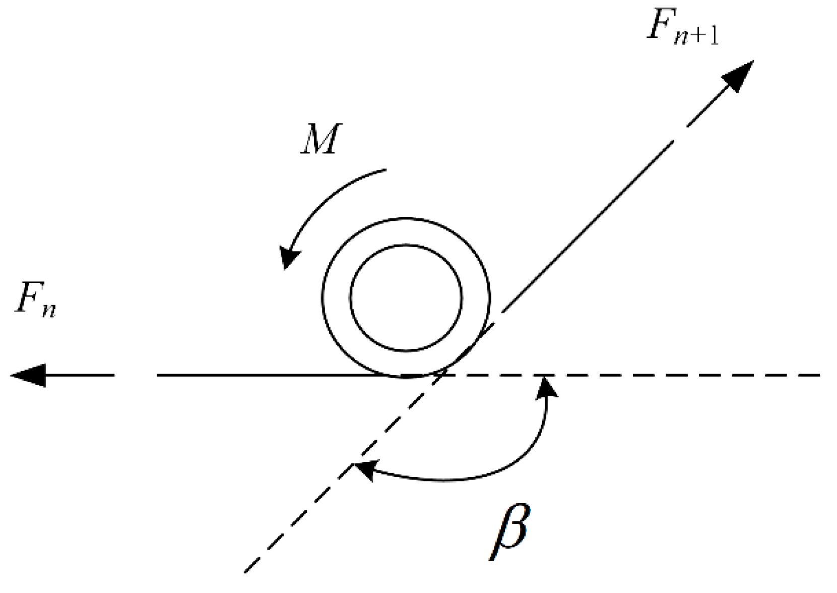
3. Deployment Modelling of Truss Antenna Using Torsional Spring
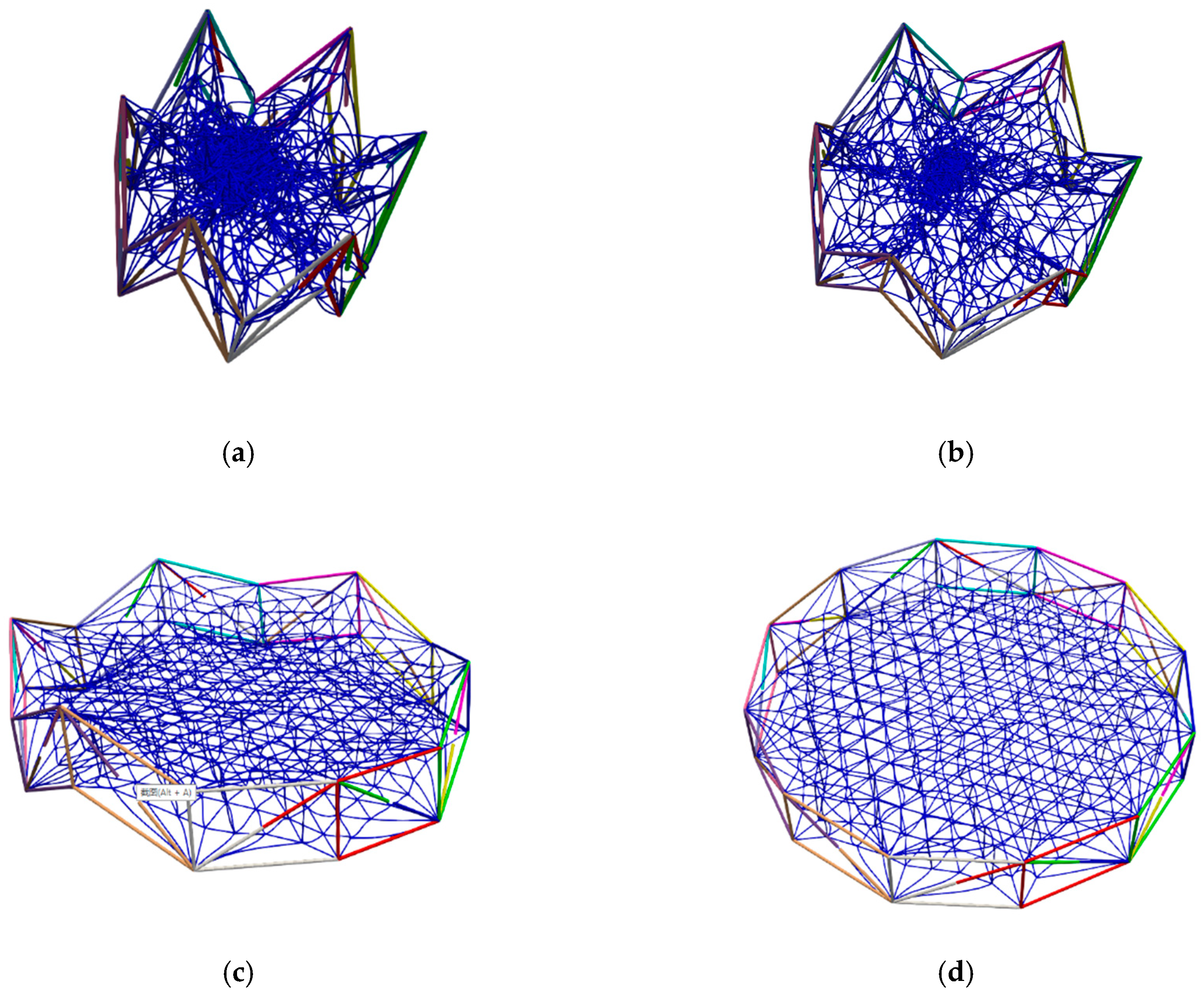
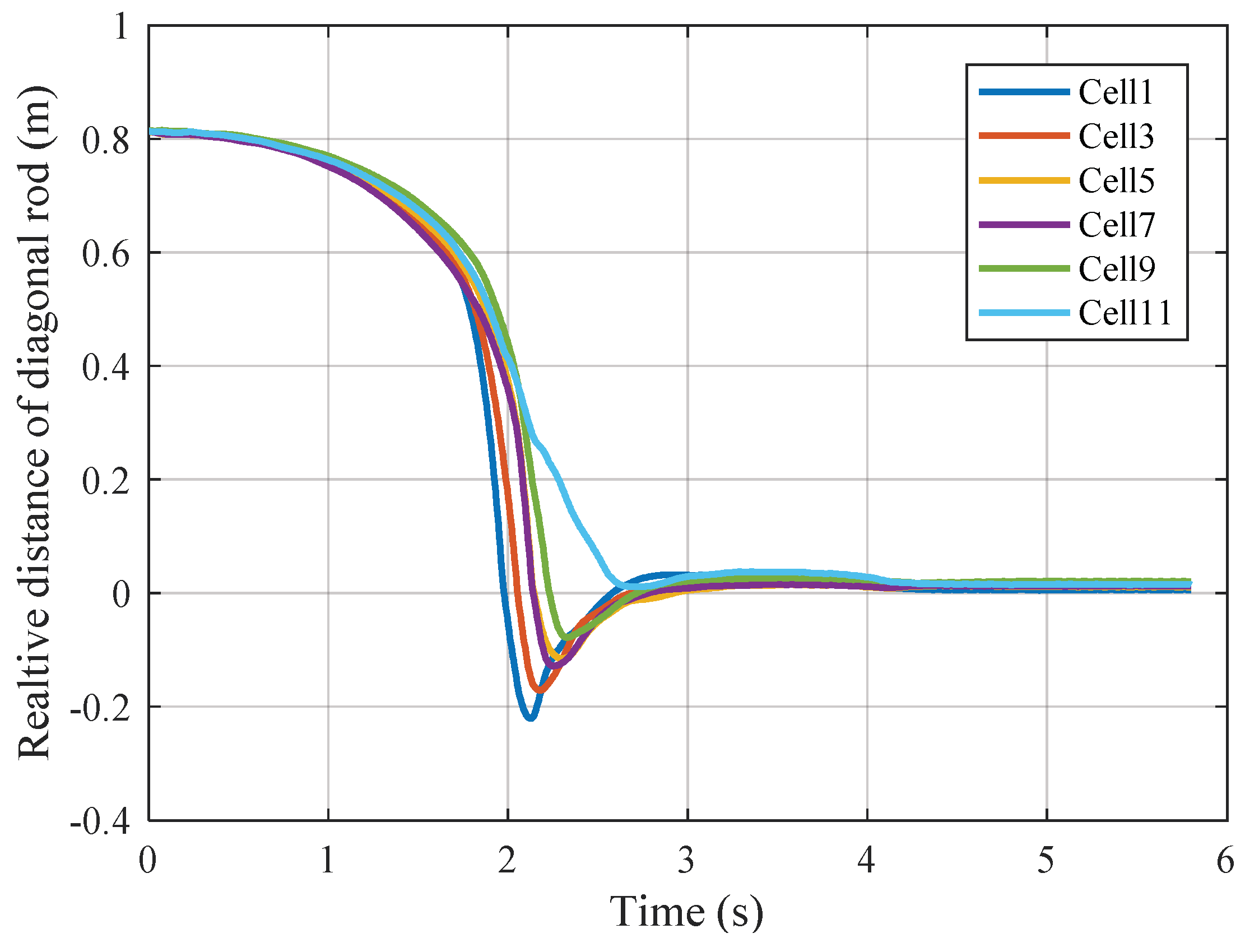
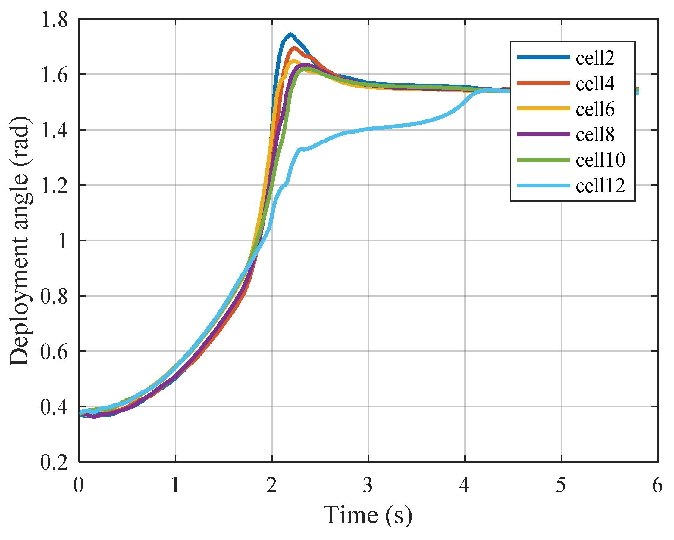
4. Dynamics Simulation of Truss Antenna
5. Conclusions
Author Contributions
Funding
Conflicts of Interest
Nomenclature
| cross-sectional area of cable | |
| damping coefficient of the torsional spring | |
| vector of constraint equations | |
| Jacobian matrix of the constraint equations | |
| generalized coordinates of cable element | |
| elastic modulus of cable | |
| frictional coefficient | |
| equivalent driving force | |
| , | driving forces on the pulley |
| synthetic moment load | |
| radial force of the bearing | |
| i | clockwise number of the cell |
| identity matrix | |
| stiffness coefficient of the torsional spring | |
| length of the vertical rod | |
| length of the horizontal rod | |
| length of the cable element | |
| equivalent mass of the truss cell | |
| mass of the cable element | |
| mass of the pulley | |
| mass matrix of the antenna system | |
| mass matrix of the cable element | |
| frictional moment | |
| number of the truss cells | |
| vector of generalized coordinates of antenna | |
| strain energy of the cable element | |
| strain energy of the cable | |
| global velocity vector of the truss | |
| local position vector of the truss | |
| vector of external forces | |
| global position vector of cable element | |
| driving force from the center of pulley to the action point | |
| global position vector of the truss | |
| shape function matrix of cable element | |
| kinetic energy of the truss | |
| kinetic energy of the cable element | |
| angle between horizontal rod and perpendicular rod | |
| angle between two body coordinate frames | |
| deployment angle | |
| Vector of the generalized coordinates | |
| Lagrange multiplier | |
| torque of the torsional spring |
References
- Shi, C.; Guo, H.; Zheng, Z.; Li, M.; Liu, R.; Deng, Z. Conceptual configuration synthesis and topology structure analysis of double-layer hoop deployable antenna unit. Mech. Mach. Theory 2018, 129, 232–260. [Google Scholar]
- Puig, L.; Barton, A.; Rando, N. A review on large deployable structures for astrophysics missions. Acta Astronaut. 2010, 67, 12–26. [Google Scholar] [CrossRef]
- Thomson, M.W. The astromesh deployable reflector. In Proceedings of the IEEE Antennas & Propagation Society International Symposium, Orlando, FL, USA, 11–16 July 1999; pp. 1516–1519. [Google Scholar]
- Meguro, A.; Harada, S.; Watanabe, M. Key technologies for high-accuracy large mesh antenna reflectors. Acta Astronaut. 2003, 53, 899–908. [Google Scholar] [CrossRef]
- Sun, Y.; Zhang, W.; Wu, R. Analysis on nonlinear dynamics of circular truss antennae in 6D systems. Appl. Math. Mech. 2019, 40, 282–301. [Google Scholar]
- Liu, L.; Shan, J.; Zhang, Y. Dynamics modeling and analysis of spacecraft with large deployable hoop-truss antenna. J. Spacecr. Rocket. 2016, 53, 471–479. [Google Scholar] [CrossRef]
- Guo, H.W.; Zhang, J.; Liu, R.Q.; Deng, Z.Q.; Cao, D.Q. Nonlinear dynamics analysis of joint dominated space deployable truss structures. J. Harbin Inst. Technol. 2013, 20, 68–74. [Google Scholar]
- Jin, S.A.M. Deployment analysis of large space antenna using flexible multibody dynamics simulation. Acta Astronaut. 2000, 47, 19–26. [Google Scholar]
- Liang, C.; Guan, F.; Zhang, H. Deployment experiment of deployable truss antenna. Chin. J. Sp. Sci. 2010, 30, 79–84. [Google Scholar]
- Li, P.; Ma, Q.; Song, Y.; Liu, C.; Tian, Q.; Ma, S.; Hu, H. Deployment dynamics simulation and ground test of a large space hoop truss antenna reflector. Sci. Sin. Phys. Mech. Astron. 2017, 47, 104602. [Google Scholar] [CrossRef]
- Li, T. Deployment analysis and control of deployable space antenna. Aerosp. Sci. Technol. 2012, 18, 42–47. [Google Scholar] [CrossRef]
- Lv, Y.; Shi, Q.; Wang, G.; Liu, F.; Xu, Y.; Li, G.; Zou, X.J. Dynamic finite-element simulation on the phased array radar antenna multiplex damage by fragment and shock wave. In Proceedings of the 2012 International Conference on Quality, Reliability, Risk, Maintenance, and Safety Engineering, Chengdu, China, 15–18 June 2012; pp. 929–933. [Google Scholar]
- Zhang, Y.; Li, N.; Yang, G.; Ru, W. Dynamic analysis of the deployment for mesh reflector deployable antennas with the cable-net structure. Acta Astronaut. 2017, 131, 182–189. [Google Scholar] [CrossRef]
- Nie, R.; He, B.; Zhang, L.; Fang, Y. Deployment analysis for space cable net structures with varying topologies and parameters. Aerosp. Sci. Technol. 2017, 68, 1–10. [Google Scholar] [CrossRef]
- Cammarata, A.; Sinatra, R.; Rigano, A.; Lombardo, M.; Maddio, P.D. Design of a large deployable reflector opening system. Machines 2020, 8, 7. [Google Scholar] [CrossRef] [Green Version]
- Shabana, A.A.; Mikkola, A.M. Use of the finite element absolute nodal coordinate formulation in modeling slope discontinuity. J. Mech. Des. 2003, 125, 357–387. [Google Scholar] [CrossRef]
- Li, B.; Qi, X.; Huang, H.; Xu, W. Modeling and analysis of deployment dynamics for a novel ring mechanism. Acta Astronaut. 2016, 120, 59–74. [Google Scholar] [CrossRef]
- Ambrósio, J.A.C.; Neto, M.A.; Leal, R.P. Optimization of a complex flexible multibody systems with composite materials. Multibody Syst. Dyn. 2007, 18, 117–144. [Google Scholar] [CrossRef] [Green Version]
- Masashi, I. Effects of coordinate system on the accuracy of corotational formulation for Bernoulli-Euler’s beam. Int. J. Solids Struct. 1994, 31, 2793–2806. [Google Scholar] [CrossRef]
- Simo, J.C.; Fox, D.D.; Rifai, M.S. On a stress resultant geometrically exact shell model. Part I: Formulation and optimal parametrization. Comput. Methods Appl. Mech. Eng. 1989, 73, 53–92. [Google Scholar] [CrossRef]
- Hughes, T.J.R.; Cottrell, J.A.; Bazilevs, Y. Isogeometric analysis: CAD, finite elements, NURBS, exact geometry and mesh refinement. Comput. Methods Appl. Mech. Eng. 2005, 194, 4135–4195. [Google Scholar] [CrossRef] [Green Version]
- Shabana, A.A.; Christensen, A.P. Three-dimensional absolute nodal co-ordinate formulation: Plate problem. Int. J. Numer. Methods Eng. 1997, 40, 2775–2790. [Google Scholar] [CrossRef]
- Li, T.; Wang, Y. Deployment dynamic analysis of deployable antennas considering thermal effect. Aerosp. Sci. Technol. 2009, 13, 210–215. [Google Scholar] [CrossRef]
- Tao, C.; Liu, L.; Zhou, Z.; Tian, Q.; Xing, Z. Analysis on non-synchronous deployment of hoop truss antenna (in chinese). Chin. Sp. Sci. Technol. 2015, 35, 1–8. [Google Scholar]
- Liu, L.; Shan, J.; Tao, C.; Cao, P.; Zhou, Z. Simulation of non-synchronous deployment of the large deployable hoop truss antenna. In Proceedings of the 2nd AIAA Spacecraft Structures Conference, Kissimmee, FL, USA, 5–9 January 2015. [Google Scholar]
- Lu, S.; Qi, X.; Hu, Y.; Li, B.; Zhang, J. Deployment dynamics of large space antenna and supporting arms. IEEE Access 2019, 7, 69922–69935. [Google Scholar] [CrossRef]
- Li, P.; Liu, C.; Tian, Q.; Hu, H.; Song, Y. Dynamics of a deployable mesh reflector of satellite antenna: Parallel computation and deployment simulation. J. Comput. Nonlinear Dyn. 2016, 11, 61005. [Google Scholar] [CrossRef]
- Peng, Y.; Zhao, Z.; Zhou, M.; He, J.; Yang, J.; Xiao, Y. Flexible multibody model and the dynamics of the deployment of mesh antennas. J. Guid. Control Dyn. 2017, 40, 1499–1506. [Google Scholar] [CrossRef]
- Du, X.; Du, J.; Bao, H.; Sun, G. Deployment analysis of deployable antennas considering cable net and truss flexibility. Aerosp. Sci. Technol. 2018, 82–83, 557–565. [Google Scholar] [CrossRef]

| Parameters | Value | Parameters | Value |
|---|---|---|---|
| Length of horizontal rods | 1 m | Truss cell number | 12 |
| Length of vertical rods | 1.2 m | Density of rod | 2700 Kg/m3 |
| Diameter of rod | 0.025 m | Elastic modulus of rod | 75 Gpa |
| Diameter of cable net | 0.005 m | Cable density | 1430 Kg/m3 |
| Number of cable elements | 1650 | Cable elastic modulus | 12 Mpa |
Publisher’s Note: MDPI stays neutral with regard to jurisdictional claims in published maps and institutional affiliations. |
© 2020 by the authors. Licensee MDPI, Basel, Switzerland. This article is an open access article distributed under the terms and conditions of the Creative Commons Attribution (CC BY) license (http://creativecommons.org/licenses/by/4.0/).
Share and Cite
Jiang, X.; Bai, Z. Dynamics Modelling and Simulation for Deployment Characteristics of Mesh Reflector Antennas. Appl. Sci. 2020, 10, 7884. https://doi.org/10.3390/app10217884
Jiang X, Bai Z. Dynamics Modelling and Simulation for Deployment Characteristics of Mesh Reflector Antennas. Applied Sciences. 2020; 10(21):7884. https://doi.org/10.3390/app10217884
Chicago/Turabian StyleJiang, Xin, and Zhengfeng Bai. 2020. "Dynamics Modelling and Simulation for Deployment Characteristics of Mesh Reflector Antennas" Applied Sciences 10, no. 21: 7884. https://doi.org/10.3390/app10217884