2. Methodology
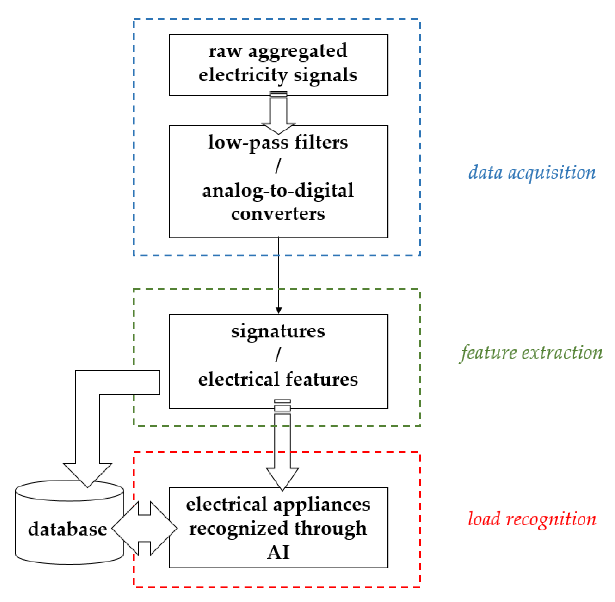
Figure 1 describes a basic (eventless) NIALM process consisting of (1) data acquisition: composite electric energy consumption data are measured by a single minimal set of plug-panel current and voltage sensors and digitized for further analysis of load disaggregation; (2) feature extraction: electrical features are extracted as feature data from digitized composite electric energy consumption data for concerned electrical appliances; and (3) load recognition: artificial intelligence (AI) is utilized to recognize extracted electrical features for concerned electrical appliances—their electric demand based on past trends can be predicted. The NIALM investigated in this paper is an eventless NIALM approach. AI conducted in the NIALM is parallel computing accelerated evolutionary computing. The basic NIALM problem can be formulated as follows:
If (1)
P(
t) stands for used composite power consumption acquired at time
t and (2)
Pi(
t) accounts for real power absorbed by concerned electrical appliance
i (profiling concerned electrical appliances and base load is done in advance), the total power consumption,
P(
t) (=
y(
t)), in an electric power distribution system can be expressed as Equation (1). In Equation (1), the summation of superimposed absorptions Σ
xi(
t)
Pi(
t) with an unmonitored base load
Pbase(
t) is made. In Equation (1),
N is the total number of concerned electrical appliances and
xi(
t), a unit value from {0, 1}, is the on/off operational status of electrical appliance
i at time
t. NIALM is used to recognize the unknown (possible) operational status of concerned electrical appliances
xi(
t)|
i = 1, 2, ...,
N at time
t when
P(
t) (=
y(
t)) acquired and given with
Pbase(
t) is known: [
x1(
t),
x2(
t), ...,
xi(
t), ...,
xN(
t)] =
F(
y(
t)) where
F is a function that returns the best
N estimates of
xi(
t) at time
t for concerned individual
N electrical appliances.
F above can be any AI algorithm. In this paper, we conduct evolutionary computing, GA, to metaheuristically search for the optimal load combinations
xi(
t) of concerned electrical appliances when acquired total power consumption
P(
t) with base load
Pbase(
t) is given at time
t (in Equation (1), profiling concerned electrical appliances to get
Pi(
t) and statistically computing base load for
Pbase(
t) from unmonitored electrical appliances is done prior.
In this paper, NIALM is declared as a combinatorial optimization problem, which is formulated as the objective metric in Equation (2) and solved by a parallel computing accelerated GA.
where
.
In Equation (2), Pi (=mean(Pi(t))) obtained in advance involves profiling each of concerned electrical appliances based on historical data. That is, Pi(t), in Equation (1), or Pi, in Equation (2), accounts for the real power that was absorbed by electrical appliance i and statistically computed for load disaggregation. Pbase, in Equation (2), from Pbase(t), in Equation (1), is defined in a similar sense, and its standard deviation can be considered. In Equation (2), τi, a tolerance term for Pi, is considered, where std(Pi(t)) is a function that returns the standard deviation of its input elements Pi(t) from historical data and ci is a constant that can be designed as a time-dependent parameter.
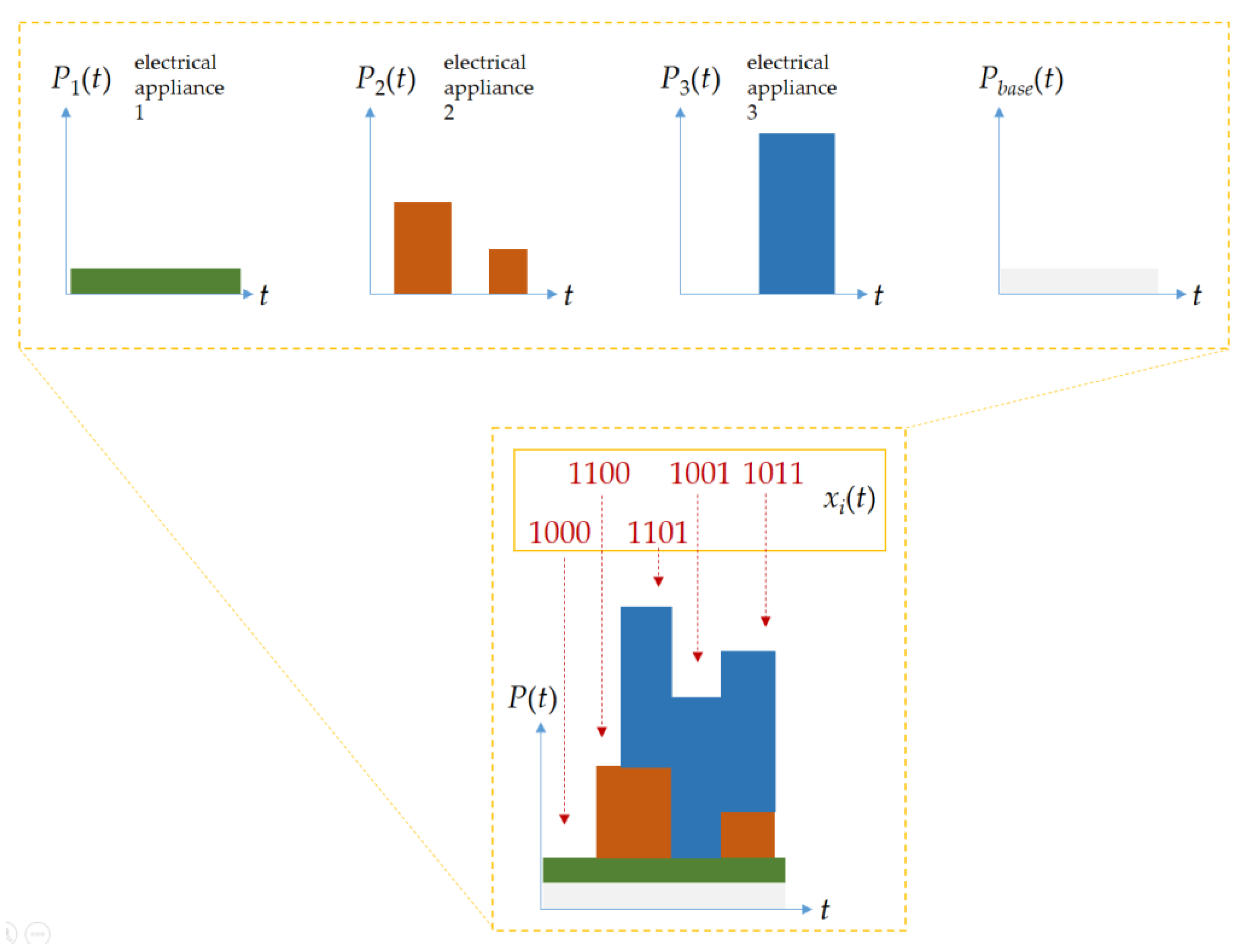
Figure 2 illustrates the principle of combinatorial search for load combinations with
xi(
t) in Equation (2) for load disaggregation, which aims to optimize load combinations by
xi(
t). In
Figure 2,
Pi(
t) represents the assumed power demand of the
i-th electrical appliance.
xi(
t) associated with
Pi(
t) is represented as a binary vector, evolved through metaheuristics, and used to minimize Equation (2) (the minimal error,
err(
t), to be obtained for load disaggregation) between the summation of superimposed absorptions Σ
xi(
t)
Pi(
t) with an unmonitored base load
Pbase(
t) and the total load
P(
t) (
P(
t) to be approximated from a pack of
Pi(
t) with
Pbase(
t)). A metaheuristic algorithm, GA, is suitable for load disaggregation formulated in Equation (2) (the objective metric is the metric we are trying to optimize and the fitness metric is the algorithm’s guide to doing so), where concerned electrical appliances are recognized by parallel computing accelerated GA for the declared objective metric. Concerned electrical appliances are constant or time-varying resistive, inductive, or capacitive loads.
The NIALM investigated in this paper has the main objective of recognizing concerned electrical appliances for (residential) DSM according to a composition of appliance-level real power consumption, which is disaggregated from total real power consumption acquired apart for load disaggregation. That is, with the minimum in Equation (2), acquired total real power consumption is the total of real power consumption by all individual electrical appliances concerned and operated where a base load should be considered. To Equation (2), a parallel computing accelerated GA as a load recognizer for load recognition of the NIALM in this paper is used to recognize the correct
xi(
t) to gain the minimum between the acquired total real power consumption and the sum of superimposed real power consumption by concerned electrical appliances. In this paper, real power consumption,
P, is extracted, as the electrical feature for load recognition in
Figure 1, from acquired total real power consumption, which is disaggregated into appliance-level real power consumption through the parallel computing accelerated GA-based NIALM of Equation (2). Concerned electrical appliances to be recognized can be constant or time-varying resistive, inductive, and capacitive loads [
4,
25].
2.1. GA-Based NIALM
GAs are a stochastic, population-based metaheuristic optimization (search) algorithm that can search for the global (quasi-)optimal solution metaheuristically to both constrained and unconstrained, NP-hard/NP-complete discrete or continuous optimization problems addressed, through (natural) selection operations that select current chromosomes for further gene recombination and through genetic operations involving (1) crossover operations that combine genetic information from selected parents’ chromosomes to produce new offspring and (2) mutation operations that provide genetic diversity among population members. The evolutionary cycle is based on the principle of biological evolution. GAs that operate based on the principle of biological evolution have been proven to be an effective metaheuristics technique in many optimization problems.
In GAs, genetic operations, comprising crossover and mutation operations, and evolutionary operations, implementing the driving force of evolution (natural selection/Darwinism), are involved. See [
26] for more details about a standard GA. In a GA addressing an optimization problem, a population of chromosomes as candidate solutions in a search space is evolved, from generation to generation, through genetic operations and evolutionary operations towards a global (quasi-)optimal solution. In an evolutionary cycle in a GA, a proportion of an existing population in its current generation is reproduced through selection operations and is used through crossover and mutation operations to breed a new population for the next generation. Selection operations select chromosomes based on a fitness-based selection procedure where chromosomes as candidate solutions are evaluated by a fitness function, and chromosomes with relatively high fitness are typically more likely to be selected. Also, crossover operations exchange subparts of two chromosomes, roughly mimicking the biological recombination between two haploid organisms. Finally, mutation operations randomly alter genes in some chromosomes, where an arbitrary bit of a chromosome is changed from its original state. In a GA, the population size depends on the nature of the problem addressed, but, typically, the population contains several hundreds or thousands of chromosomes/candidate solutions. Chromosomes are generated at random in the initial population. The evolutionary cycle is repeated, from generation to generation, until a termination condition such as a maximum of generations prespecified and reached has been met.
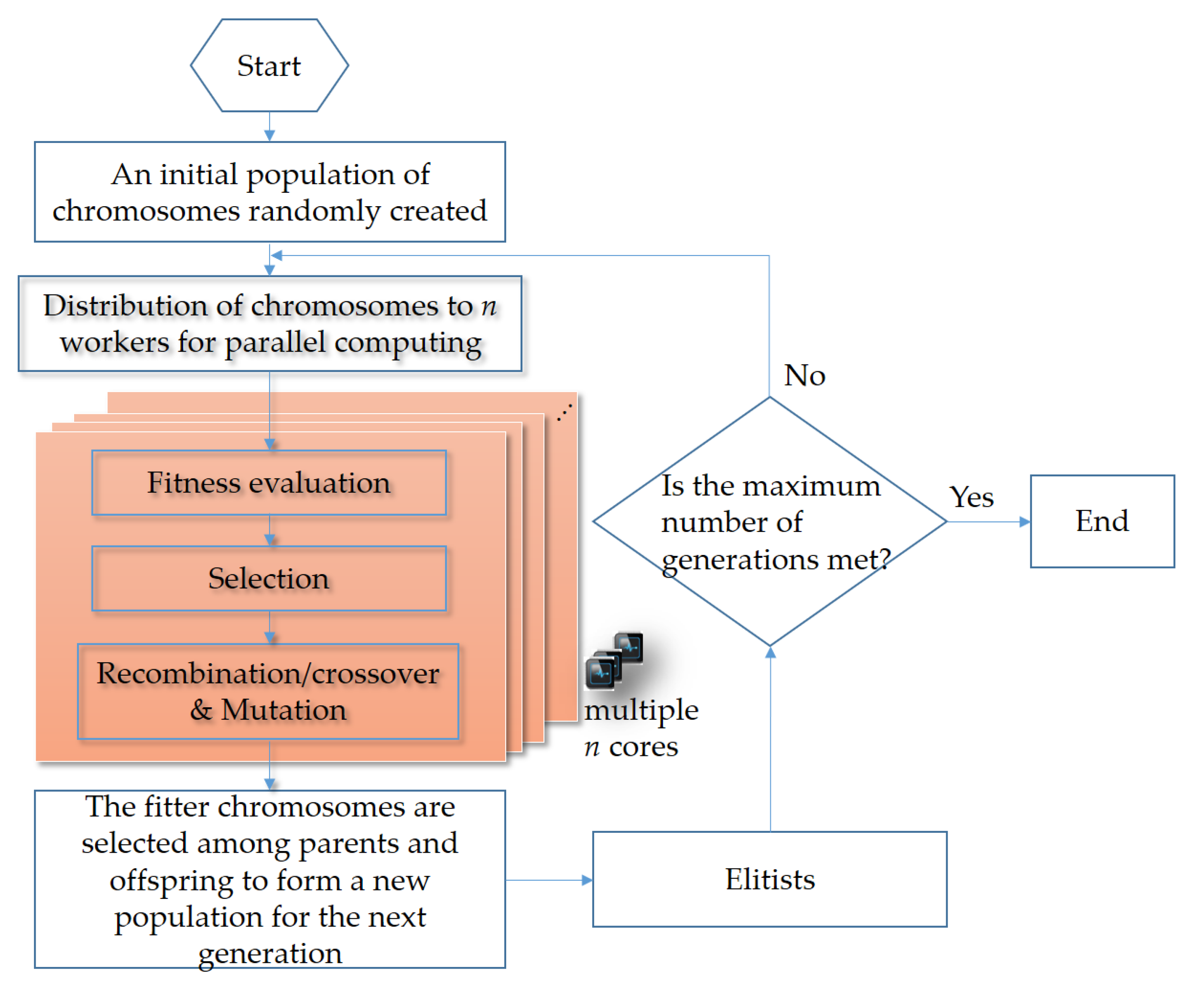
A GA used to address optimization problems is innately a parallel algorithm that can be run on a multicore processor. The workflow depicting the parallel computing accelerated GA used to solve Equation (2) for load recognition in the NIALM in this paper is shown in
Figure 3. In the GA, function evaluations are farmed out to different processors on a multicore processor; they are executed in parallel.
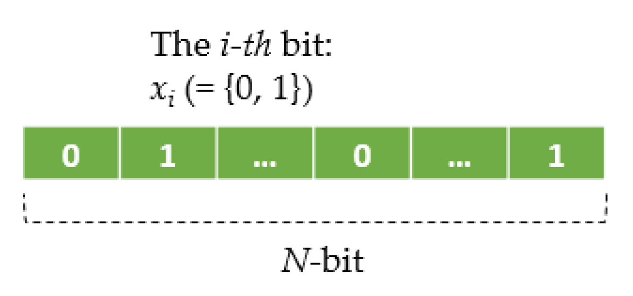
Figure 4 shows that
xi(
t) (at time
t) in Equation (2) are encoded as a chromosome for an evolutionary cycle of the GA. To evaluate a chromosome with Equation (2), the GA decodes it as a computed summation of superimposed absorptions Σ
xi(
t)
Pi(
t). With an initial population of randomly generated chromosomes that are started in the parallel computing accelerated GA in
Figure 3, successive generations are constructed through evolution. Fitter chromosomes are more likely to survive, based on selection, and to participate in genetic operations [
27]. Here, (1) a roulette selection strategy choosing parents by simulating a roulette wheel in which the area of the section of the wheel corresponding to an individual is proportional to the individual’s expectation associated with its scaled fitness value is conducted (a ranking method that scales raw fitness values based on the rank of each individual rather than its raw fitness value is used for fitness scaling), (2) a single-point crossover operator is used, (3) a bit-wise mutation operator is utilized, and (4) an elitist strategy guaranteeing that the solution quality does not decrease during evolution is also conducted.
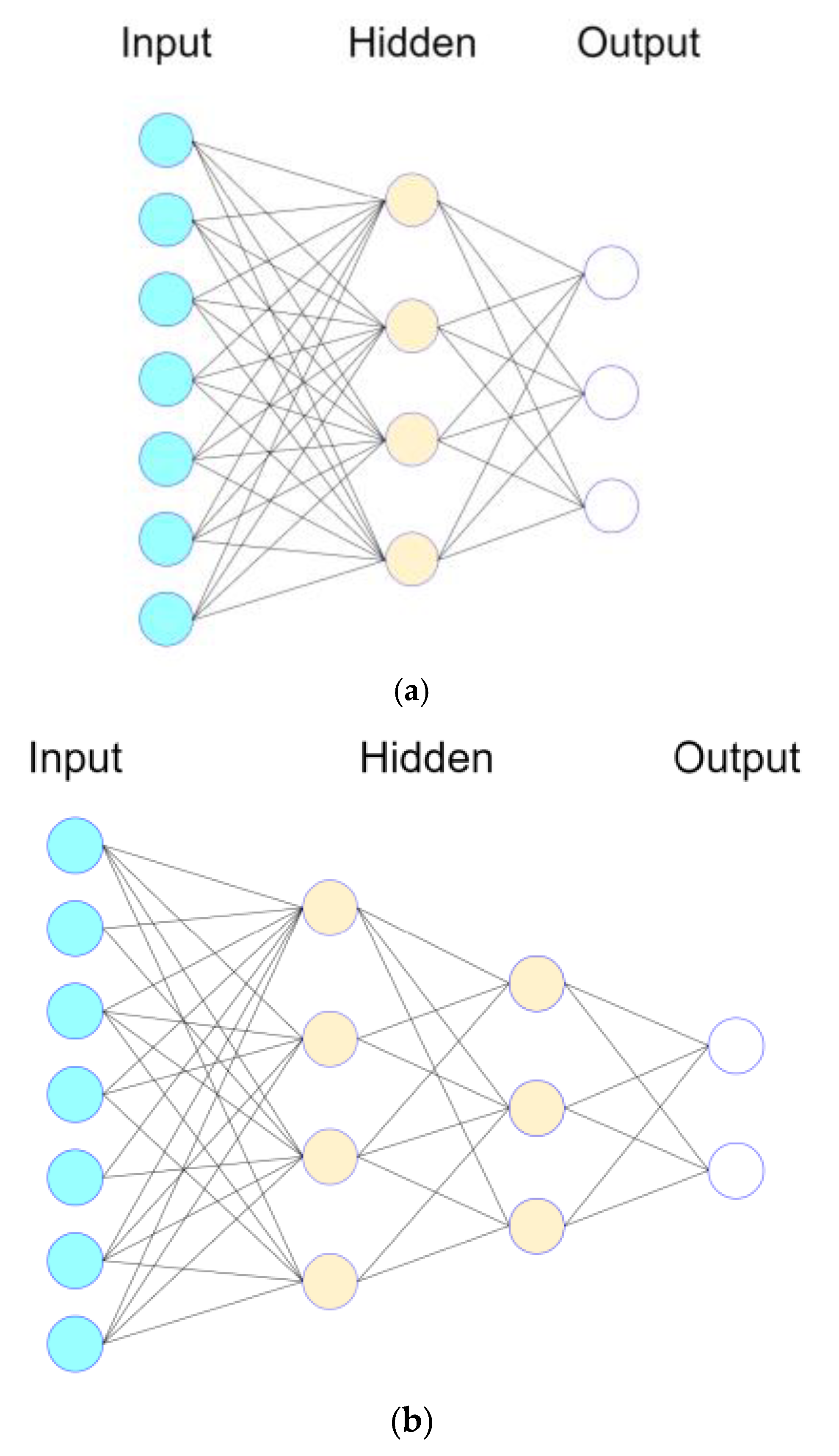
2.2. Feed-Forward, Multilayer ANN-Based NIALM
A feed-forward, multilayer ANN can be used to learn and distinguish from aggregated, extracted NIALM feature data for load disaggregation. In this paper, a comparative study where a feed-forward, multilayer ANN against the GA described in the previous subsection is used to address the same NIALM/load disaggregation problem, Equation (1), is conducted. As seen in
Figure 5, a feed-forward, multilayer ANN contains an input layer, a number of intermediate hidden layers, and an output layer. The size of the input layer depends on the number of independent variables (extracted representative features) of considered feature data to be learned. The number of intermediate hidden layers with their size (the number of hidden neurons) specified in each hidden layer, can be determined experimentally through hyperparameter tuning where hyperparameters including the learning algorithm and the number of epochs for iterative rounds of learning affect how well the connectionism can represent the considered feature data (the hyperparameters are a set of parameters whose value is specified and used to control the learning process). The size of the output layer depends on the number of dependent variables (mutually exclusive classes) of considered feature data to be fitted.
In this paper, F1 score described in detail in the following subsection is conducted and used as the performance metric to indicate the effectiveness of the two parallel computing-accelerated AI approaches in load recognition for load disaggregation.
2.3. Performance Evaluation of Load Recognition by F1 Score
In this paper, as shown in Equation (3),
F1 score [
29] is used to evaluate the performance of the two parallel computing-accelerated AI approaches in load recognition for load disaggregation.
In Equation (3), precision is a ratio of the total number of correctly recognized positives to the total number of predicted positives. Recall (i.e., sensitivity or hit rate) is a ratio of the total number of correctly recognized positives to the total number of actual positives. See ref. [
29] for more details about precision and recall. To summarize,
F1 score is the harmonic mean of precision and recall. A recognizer that produces no false positives has a precision of 1.0. A recognizer that produces no false negatives has a recall of 1.0. In Equation (3), an
F1 score reaches its best value at 1.0 (perfect precision and recall). The higher the score, the better the recognition performance. Besides
F1 score, we also use receiver operating characteristic (ROC) curves [
29] to evaluate the performance of the two parallel computing-accelerated AI approaches in load recognition for load disaggregation. An ROC curve considering false positive rate (FPR) and true positive rate (TPR) is a graph showing the recognition performance of a recognizer examined at all recognition thresholds (or with different configuration settings) [
29]. In an ROC curve, an error to a trained and validated recognizer can be computed by the Euclidean distance, from the perfect identification (FPR = 0, TPR = 1) til a resulting (FPR, TPR) [
30,
31] where FPR and TPR are defined as Equations (4) and (5), respectively. TPR is referred to as recall. As seen in Equations (4) and (5), ROC curves [
29] are also used to evaluate the performance of the investigated methodology in load recognition, where TPR (a synonym for recall) defined in Equation (4) and FPR defined in Equation (5) are considered. See ref. [
29] for more details about precision and recall.
In Equations (4) and (5), TP (true positives) means the data instances are recognized, and fit with reality. TN (true negatives) means the data instances are recognized, and the nonexistence fits with reality. FP (false positives) means the data instances are erroneously recognized as positives. Finally, FN (false negatives) means the data instances are incorrectly recognized as negatives.
3. Experimentation and Results
In this section, experiments are carried out to verify the validity of the investigated NIALM, by a publicly available UK-DALE (UK Domestic Appliance-Level Electricity) dataset [
32]. The UK-DALE dataset contains records of power consumption measured and collected from five different households in the UK. In each house, the authors in [
32] recorded both whole-house power consumption (power demand) from the mains every 6 s and power consumption by concerned individual electrical appliances every 6 s.
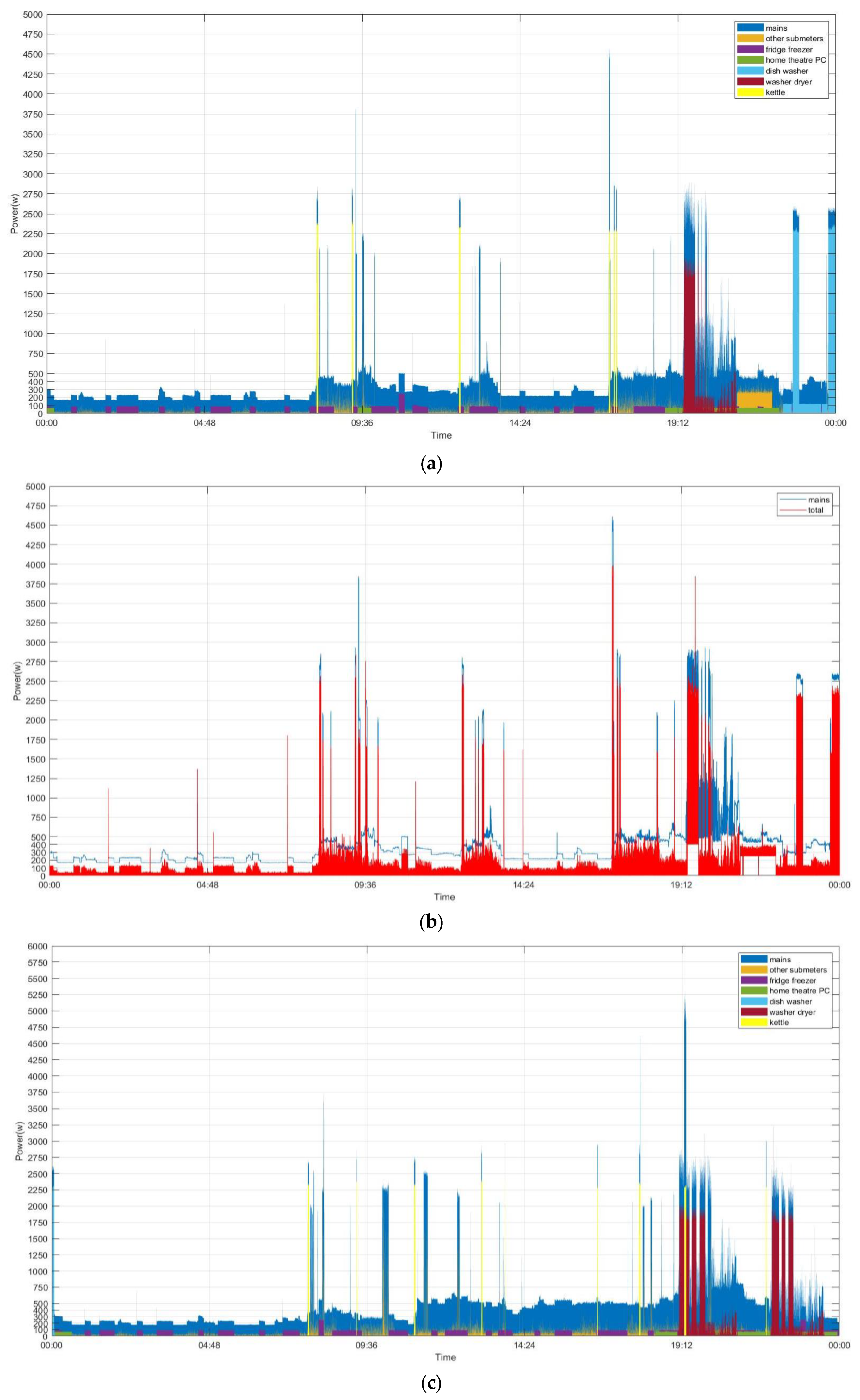
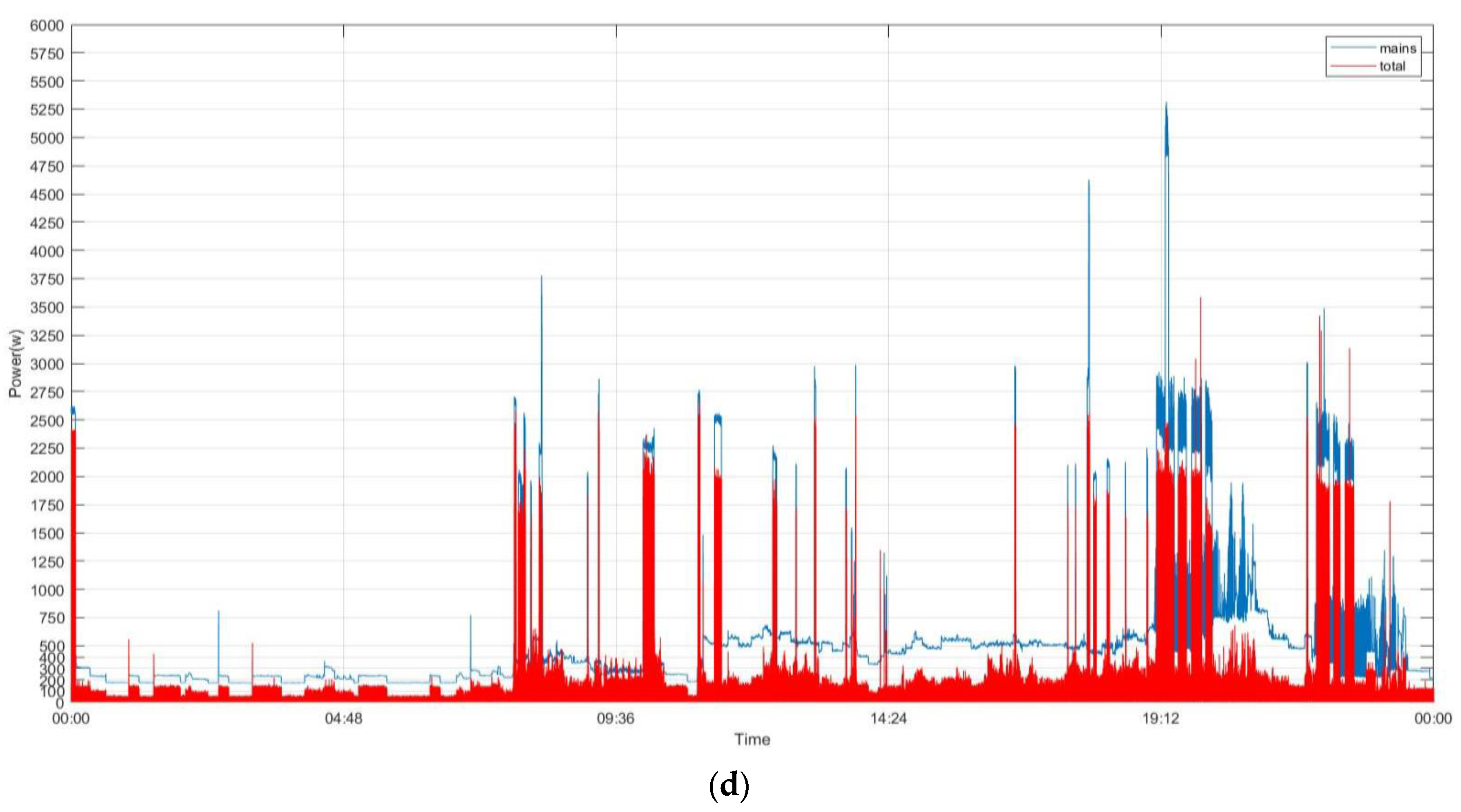
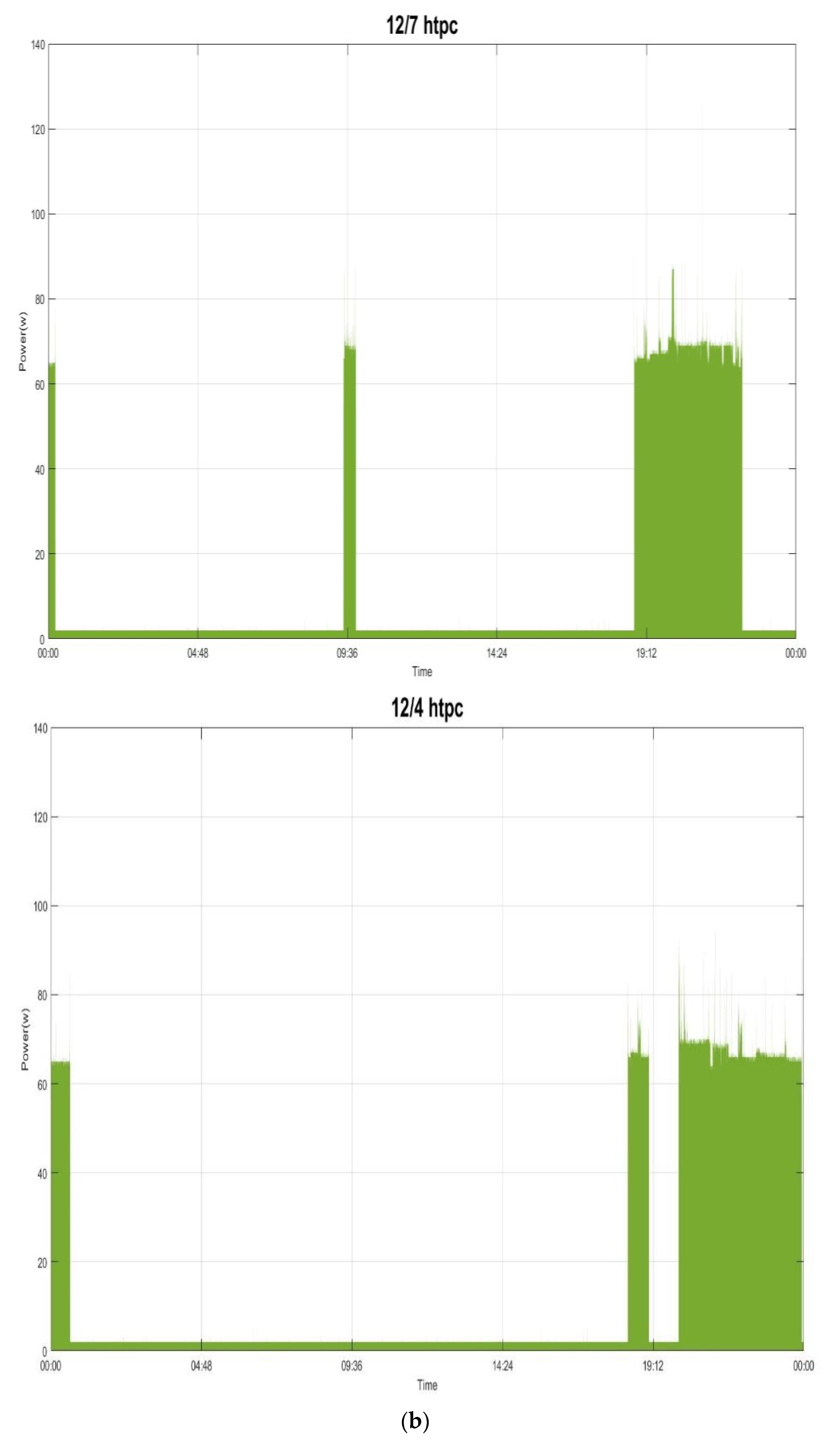
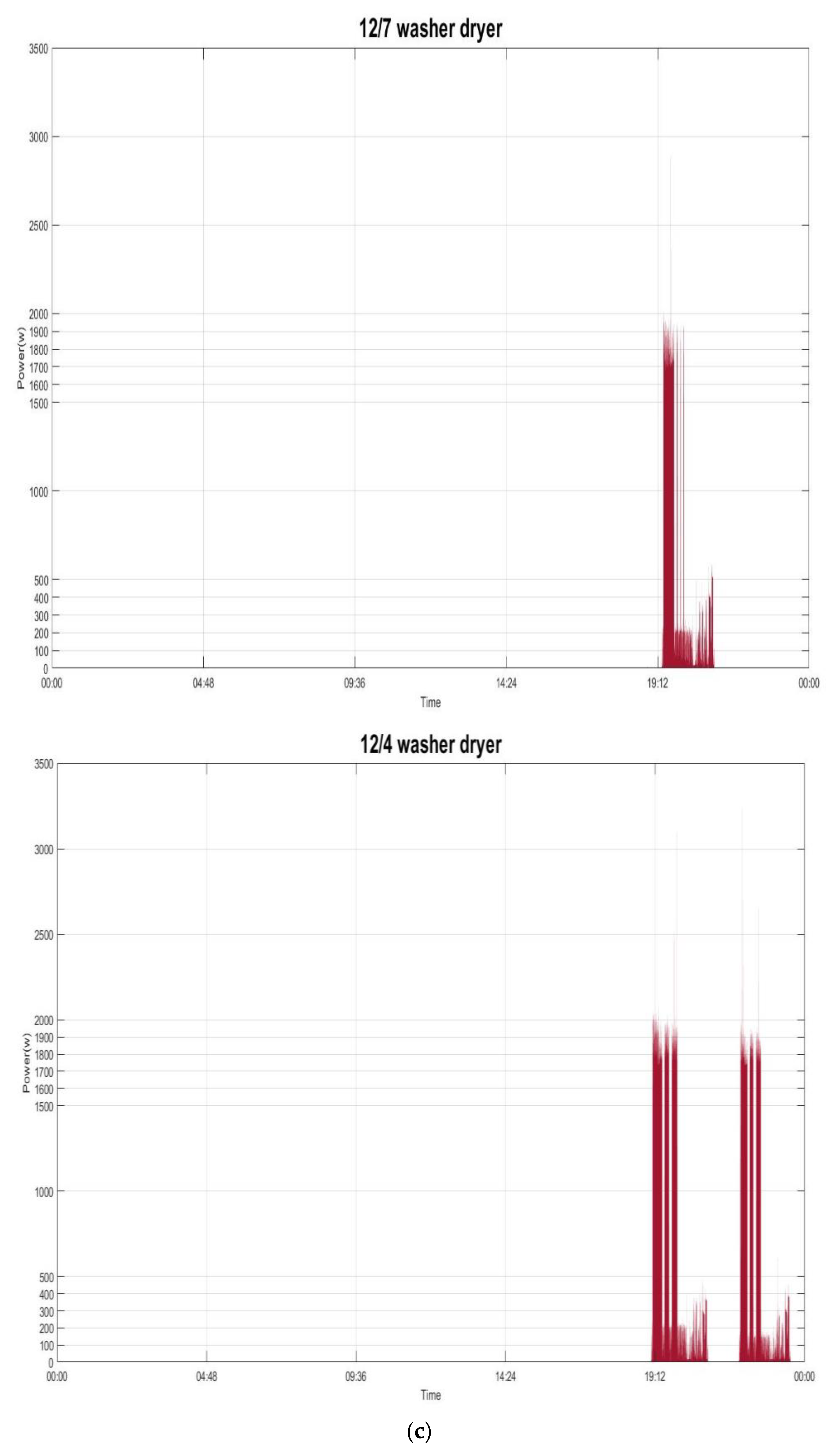
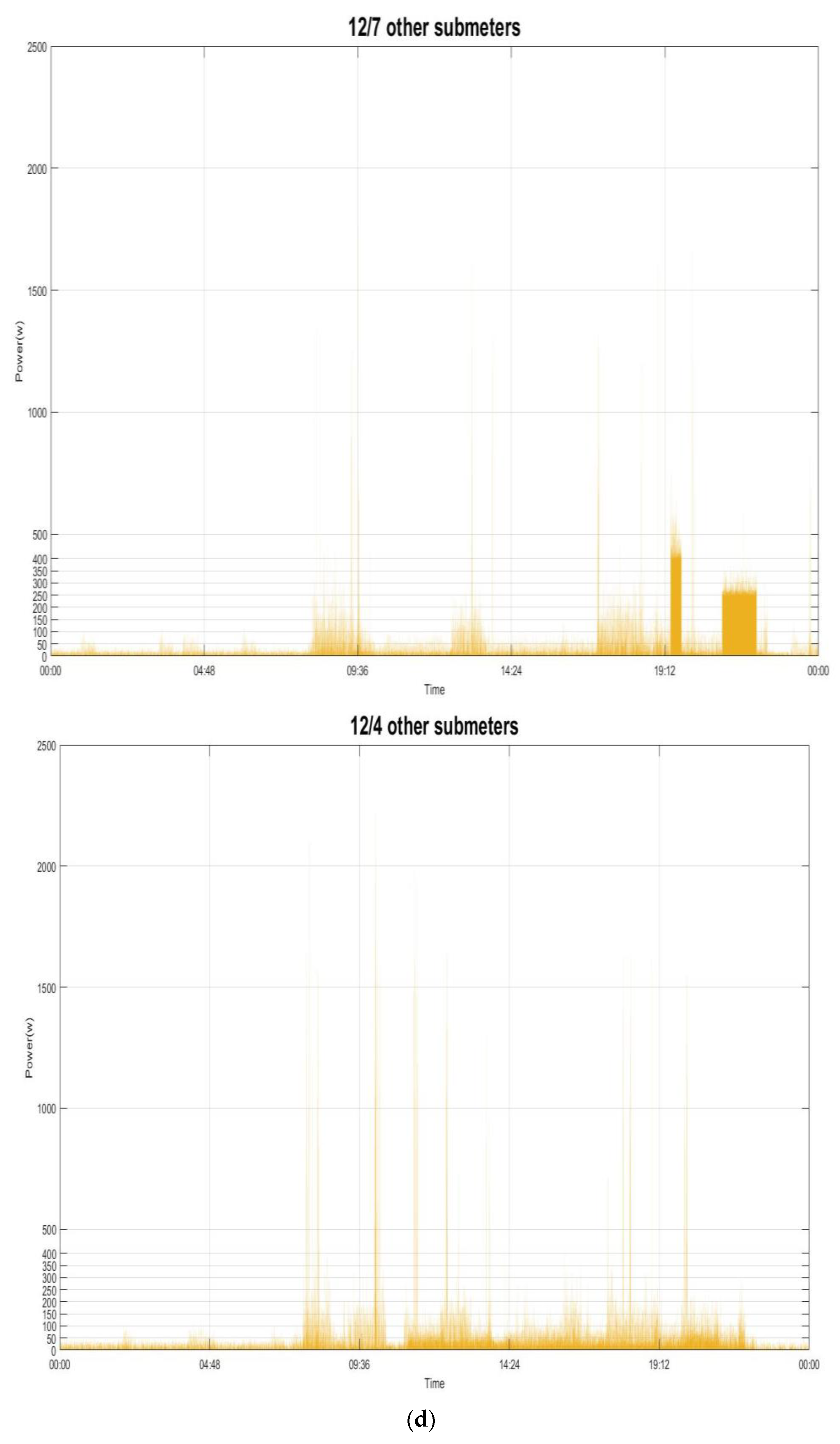
Figure 6 shows the considered historical power demand on two typical days (Sunday 7 December 2014 (
Figure 6a,b) and Thursday 4 December 2014 (
Figure 6c,d)) in House 1 from the UK-DALE dataset, which is considered, parsed, and used to experimentally validate the performance of the investigated methodology in load recognition. The summarization of the UK-DALE dataset can be found in [
32]. In
Figure 6a,c, we show the total power demand in the mains. Also, we show the power demand by the concerned individual electrical appliances and all other submeters [
32] considered together and treated as a single individual in power absorptions for load disaggregation. As shown in
Figure 6b,d, the thin white gap between the power demand in the mains and the summed-up power demand illustrates the amount of power demand, base load, which is not concerned/metered. The concerned electrical appliances, including the considered submeters as a single individual in power absorptions to
Pi in Equation (2), are listed in
Table 1; their power demand is shown in
Figure 6 and the base load,
Pbase in Equation (2), is assumed to have a constant value of 150.0 watts for simplicity’s sake.
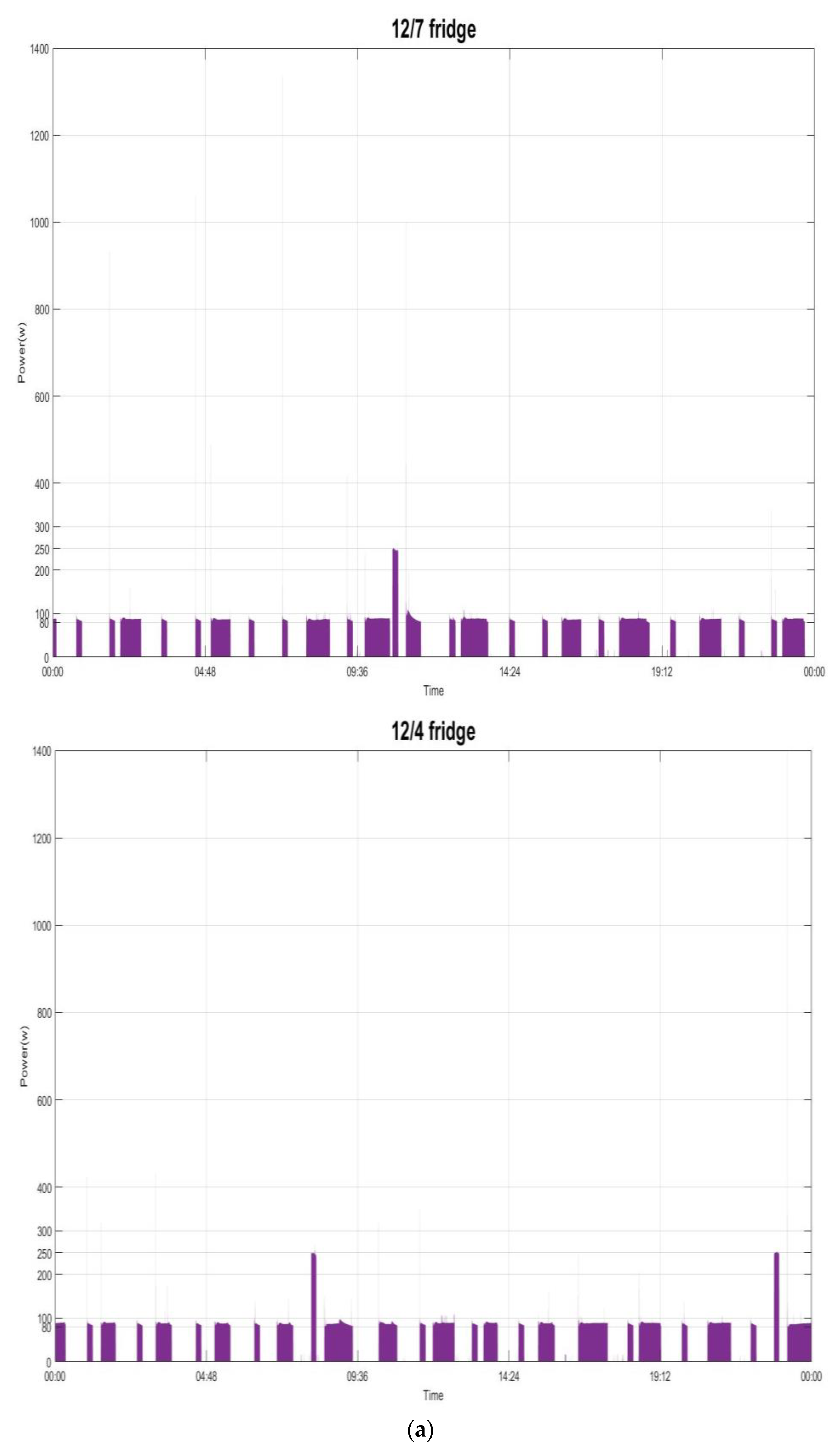
Figure 7 shows the power demand of the several individual electrical appliances targeted in this paper and listed in
Table 1. The behavior of the power demand by the electrical appliances can be found in [
32]. For example,
Figure 7a shows the power demand by the fridge running and doing its respective job of compressor on (state 1: its mean power consumption is ~90.0 watts with a standard deviation of ~44.0) or defrost (state 2: its mean power consumption is ~245.0 watts with a standard deviation of ~16.0). In this paper, the load classes considered from the targeted electrical appliances in
Table 1 and recognized are shown in
Table 2.
We used the UK-DALE dataset [
32] as our reference dataset to experimentally validate the performance of the investigated methodology in load recognition; note that, in the dataset, data that were recorded from House 1 in the UK were considered in this experiment. In this experiment, a total of 4096 (=2
N(=12)) load combinations need to be recognized by the parallel computing accelerated GA in this paper (the total number of meters installed and used as ground truth in the house environment is 54 [
32]), where a total of 208 composite power consumption (NIALM) data instances are disaggregated according to Equation (2). For each data instance acquired at time
t and disaggregated, the parallel computing accelerated GA indicates the electrical appliances whose operation is active or inactive. In this experiment, the parallel computing accelerated GA is implemented in MATLAB
® and run on an Acer Predator G3-710 Intel
® Core
TM i7-6700 CPU (3.40 GHz) (RAM: 16 GB) personal computer (PC), where for parallel computing the total number of available workers,
n, on the machine is four. Note that running the parallel computing accelerated GA requires Global Optimization Toolbox™ [
33] required with Parallel Computing Toolbox™ [
34] for parallel computing. In this experiment, for simplicity,
ci in Equation (2) is set to 1.5, which can be determined through an exhaustive search for the house environment. Also,
Pbase assumed and estimated according to
Figure 6b,d is 150.0 watts. Parameters for the parallel computing accelerated GA are specified below. The population size,
pop_size, is 250. The initial population is created randomly in bit strings, where the total length of each chromosome is 12. The roulette selection strategy is used, and for this proportional selection procedure raw fitness values based on the rank of evaluated chromosomes, rather than their raw fitness value, are scaled. The single-point crossover operator is conducted; the crossover fraction of the population to be evolved is 0.55. The bit-wise mutation operator is used; the mutation rate is 0.01. An elitist strategy that guarantees a total of top (0.05 ×
pop_size) chromosomes to survive from their current population to the next population is also used. The maximum number of generations is 50. Finally, the fitness function is clarified as —
E, where
E is the declared objective function shown in Equation (2).
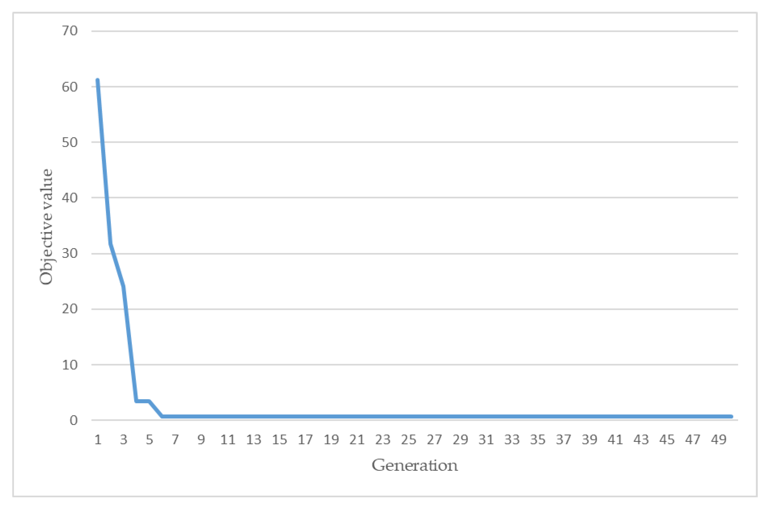
Figure 8 shows the evolutionary trajectory of the parallel computing accelerated GA to a disaggregated NIALM data instance. The resulting objective value obtained is 0.7. To the total 208 NIALM data instances where they are run over for load disaggregation, the parallel computing accelerated GA compared to a standard GA achieves, in terms of computation time, an acceleration of up to 3.49 × (=19.57 s/5.60 s).
In order to evaluate the performance of the parallel computing accelerated GA in load recognition, we examined the ROC curves, TPR and FPR in Equations (3) and (4), where their Area under ROC (AUC) is shown.
Table 3 tabulates the load recognition results obtained by the parallel computing accelerated GA applied on the class-imbalanced data, where the
F1 score is shown to each load class.
Table 4 also tabulates the load recognition results obtained by the parallel computing accelerated GA, where TPR vs. FPR is also shown to each load class. As shown in
Table 4, the presented methodology got good load recognition results (against random guesses with AUCs of 0.5) for the fridge, kettle, and dishwasher, where activities of daily living (ADLs) [
35] can be inferred from them for occupants in the house. The experimental results reported in this paper have shown the validity of the parallel computing accelerated GA-based NIALM for load disaggregation. In addition, the NIALM’s achieved acceleration of up to 3.49× has been shown. The parallel computing accelerated GA can exploit parallel computing and, thus, reduce computation time. Computation time will increase exponentially when a large amount(s) of NIALM data is run over for load disaggregation (Equation (2)) in a large-scale evaluation of NIALM. Parallel computing will be exploited massively and the computation time will, thus, be reduced drastically. As shown in
Table 3 and
Table 4, the performance of the presented methodology in load recognition needs a significant improvement, where the presented methodology suffers from similar
P where the concerned electrical appliances or the load combinations of the concerned electrical appliances are identical. It will be improved. The improvement is shown below.
The performance of the parallel computing accelerated GA in load recognition needs a significant improvement, although the algorithm is capable of recognizing the fridge/freezer, kettle, and dishwasher in the house environment for ADLs. A comparative study is conducted below, where a feed-forward, multilayer ANN as neurocomputing against evolutionary computing is used for the addressed NIALM problem. A network configuration of 1-15-12 of a feed-forward, multilayer ANN in
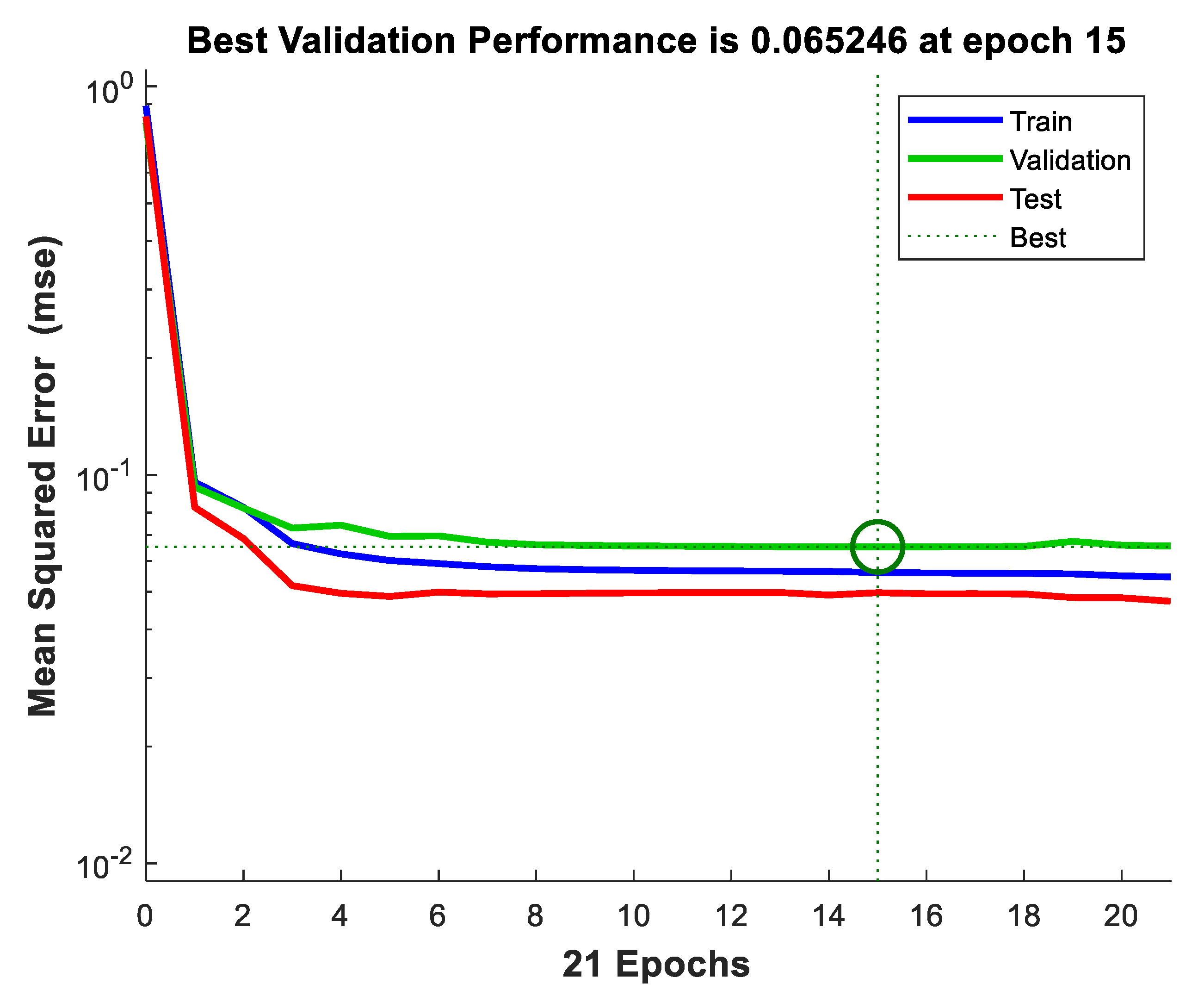
Figure 5a is constructed, specified, and used, in this experiment, to address the same 208 NIALM data instances used before. The feed-forward, multilayer ANN was trained on 135 randomly sampled training data instances (~65% of the whole dataset) and tested on the remaining 73 test data instances. The training trajectory of the constructed, specified and used feed-forward, multilayer ANN is shown in
Figure 9. The resulting mean squared error (MSE) is 0.055 (its initial MSE is 0.891).
Table 5 tabulates the load recognition results obtained by the feed-forward, multilayer ANN, which has been well trained and validated on the class-imbalanced training data. In
Table 5, the
F1 score is shown to each load class.
Table 6 also tabulates the load recognition results obtained by the well-trained and -tested feed-forward, multilayer ANN applied on the class-imbalanced test data. In
Table 6, TPR vs. FPR is also shown to each load class. The authors of [
24] used the benchmark implementations, from NILMTK in [
36], of the combinatorial optimization (CO) approach, which was developed in [
1], as a load recognizer to perform load disaggregation for the UK-DALE dataset. A comparison among the CO, the parallel computing accelerated GA, and the feed-forward, multilayer ANN for load recognition is shown in
Table 7. As shown in
Table 3,
Table 4,
Table 5,
Table 6 and
Table 7, the feed-forward, multilayer ANN outperforms, in terms of load recognition, the parallel computing accelerated GA that is slightly superior in load recognition to the CO.
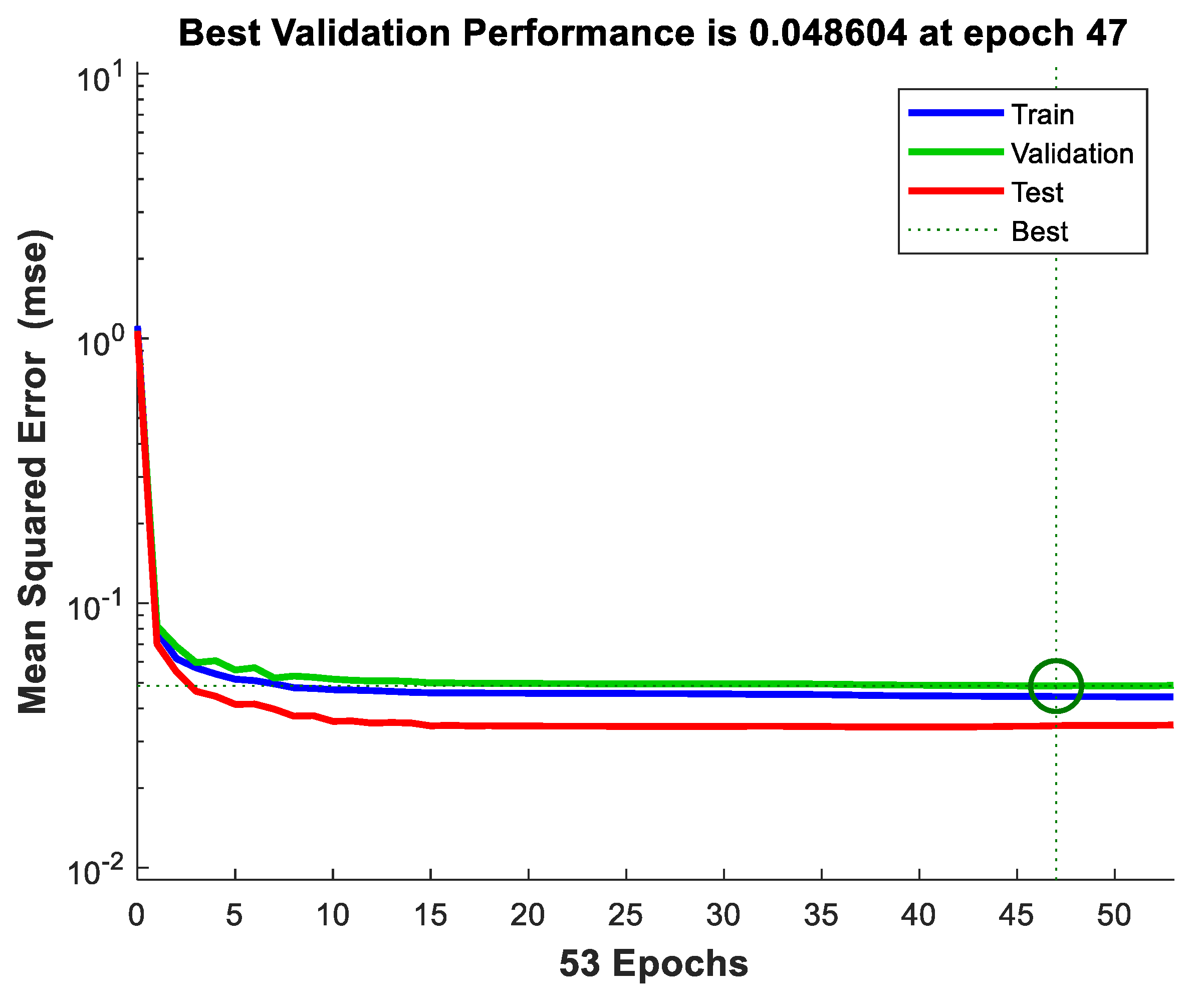
In this experiment, more NIALM data instances, a total of 989 NIALM data instances, are sampled from the house environment and used to experimentally verify the performance of a feed-forward, multilayer ANN (
Figure 5a) in terms of load recognition. A network configuration of 1-23-12 of a feed-forward, multilayer ANN was constructed, specified, and used. Also, the feed-forward, multilayer ANN was trained on 643 randomly sampled training data instances (~65% of the whole dataset) and tested on the remaining 346 test data instances. The training trajectory of the feed-forward, multilayer ANN is shown in
Figure 10. The resulting MSE was 0.044 (the initial MSE was 1.110). The feed-forward, multilayer ANN can learn from the training data instances across all available CPU workers on the PC used.
Table 8 tabulates the load recognition results obtained by the feed-forward, multilayer ANN where it has been well-trained and -validated. In
Table 8, the
F1 score is shown to each load class.
Table 9 also tabulates the load recognition results obtained by the well-trained and -validated feed-forward, multilayer ANN applied on class-imbalanced test data. In
Table 9, TPR vs. FPR is also shown for each load class.
As seen in
Table 8, the 989 NIALM data instances make up a class-imbalanced dataset. Accuracy alone is not sufficient for evaluating a recognizer trained from class-imbalanced data, where in each class there may exist a significant disparity between positives (status: On) and negatives (status: Off). As a result,
F1 score, the harmonic mean of precision and recall, is conducted and used to address the class-imbalanced problem (in order to fully evaluate the performance of the feed-forward ANN in terms of load recognition). Various metrics in addition to
F1 score have been developed.
Table 9 shows TPRs vs. FPRs, for ROC curves, obtained by the well trained and tested feed-forward, multilayer ANN applied on the class-imbalanced test data for NIALM, where one ROC curve can be shown per class (the maximum AUC is 1, which corresponds to a perfect recognizer as all positives above all negatives—100% sensitivity of no false negatives and 100% specificity of no false positives—are ranked). The authors of [
24] used two different types of ANNs, deep NNs by autoencoder and long short-term memory (LSTM), as load recognizers to perform load disaggregation for the UK-DALE dataset. Comparison among the autoencoder, the LSTM and the presented feed-forward, multilayer ANN for load recognition is shown in
Table 10. As shown in
Table 8,
Table 9 and
Table 10, the feed-forward, multilayer ANN that gives similar performance, in load recognition, against autoencoder outperforms the LSTM. The load recognizer of the presented NIALM is a shallow neural network, not a deep neural work. As reported in this section, the presented feed-forward, multilayer ANN is able to discriminate the targeted electrical appliances from the house environment well.


