Article

Time Series Forecasting of Agricultural Products’ Sales Volumes Based on Seasonal Long Short-Term Memory

Division of Computer Science and Engineering, Jeonbuk National University, Jeonju 54896, Korea
*
Author to whom correspondence should be addressed.
Appl. Sci. 2020, 10(22), 8169; https://doi.org/10.3390/app10228169
Submission received: 28 September 2020 / Revised: 7 November 2020 / Accepted: 9 November 2020 / Published: 18 November 2020
(This article belongs to the Section Computing and Artificial Intelligence)

Abstract

:
In this paper, we propose seasonal long short-term memory (SLSTM), which is a method for predicting the sales of agricultural products, to stabilize supply and demand. The SLSTM model is trained using the seasonality attributes of week, month, and quarter as additional inputs to historical time-series data. The seasonality attributes are entered into the SLSTM network model individually or in combination. The performance of the proposed SLSTM model was compared with those of auto_arima, Prophet, and a standard LSTM in terms of three performance metrics (mean absolute error (MAE), root mean squared error (RMSE), and normalization mean absolute error (NMAE)). The experimental results show that the error rate of the proposed SLSTM model is significantly lower than those of other classical methods.

1. Introduction

Agricultural commodity prices are volatile, and they are affected by various factors, including weather conditions, the planting area, consumption trends, and policy factors [1]. Price volatility makes it difficult for producers to make sales decisions, which leads to instability in producer incomes and consumer burdens on purchasing behavior. Therefore, accurate forecasting of agricultural supply and demand is essential for both agricultural producers and consumers. To reduce volatility, it is crucial to establish an agricultural production plan at the beginning of the production process by forecasting supply and demand [2,3,4]. Forecasts of the sales volumes of agricultural products can use historical time-series data to reduce risk at the production stages and reduce price fluctuations after production [5]. However, the trends of the agricultural market are complicated and nonlinear as a result of numerous factors, including economic globalization, financial speculation, climate change, and oil price fluctuations. This complexity makes it increasingly difficult to accurately predict agricultural supply and demand [1,5]. Since it is very difficult to predict agricultural supply and demand with different variability factors, more research needs to be conducted on such predictions. By contrast, studies on energy and electrical load predictions, which have less volatile factors than agricultural predictions, are actively conducted. Specifically, various studies have examined the prediction of energy and electric loads, which play an important role in energy management systems [6,7,8,9,10,11]. The studies on other applications include rainfall forecasting [12], bitcoin price forecasting [13], bankruptcy prediction [14], and stock price prediction [15,16].
Agricultural product sales are mainly time series, and many general time series forecasting methods can be applied to forecast them. The problem of predicting the supply and demand of agricultural products is mostly solved using classical statistical models or machine learning models. The machine learning models are typically implemented with recently emerging deep learning models, such as the recurrent neural network.
In this paper, we propose an agricultural sales forecasting system based on deep learning to stabilize agricultural supply and demand. The time-series data for the sales volume of agriculture products contain a high degree of weekly and monthly seasonality. The conventional models, such as seasonal autoregressive integrated moving average (SARIMA) and LSTM (long short-term memory), have the ability to model such seasonality. The SARIMA model represents the seasonal information statistically with its formulation. However, the SARIMA model has no ability to accept “explicit” seasonal information. An example of explicit seasonal information is that the current time step is May and Friday. The LSTM model is currently very popular as a deep learning model for processing various kinds of time-series data and natural languages [17]. The state transition and gate mechanisms of LSTM can implicitly capture the seasonal information in the data. We observe that the explicit seasonal information can be additionally input to LSTM through the input layer and that this idea will improve the accuracy. This observation motivates our research. The proposed LSTM model is a prediction method that adds weekly, monthly, and quarterly features to the existing LSTM method. We call the proposed LSTM model seasonal LSTM (SLSTM). The seasonality information, namely, weekly, monthly, and quarterly features, are input into the SLSTM either individually or simultaneously.
In our experiment, the forecasting performance is evaluated in terms of three error metrics: mean absolute error (MAE), root mean squared error (RMSE), and normalization mean absolute error (NMAE). The proposed SLSTM model shows a lower error rate than the conventional methods.
Section 2 presents a literature review. Section 3 describes the dataset used in our experiments. It also describes the proposed SLSTM model, along with conventional methods. Section 4 presents the experimental results and performance comparisons. Section 5 concludes the paper.

2. Literature Review

We divide the time-series prediction model into conventional statistical models, machine learning models, and hybrid models that combine both [7,18]. In general, the time scales of forecasting can be divided into three categories: short-term forecasts (from one hour up to one week), mid-term forecasts (from one month up to one year), and long-term forecasts (more than one year); these are also respectively referred to as short-term horizon, mid-term horizon, and long-term horizon. Most works use the short-term horizon since it achieves higher accuracy than the other types [7,8,19].
Conventional statistical methods include linear regression, autoregressive moving average, general exponential technique, autoregressive integrated moving average (ARIMA), and seasonal ARIMA (SARIMA) [7,8,20]. The ARIMA models, developed by Box and Jenkins [21], are the most frequently used, and these models constitute a widely used class of linear models for univariate time series. The ARIMA model relies on several criteria to identify an optimal parameter setting, leading to disadvantages of manual selection and a considerable amount of computation time [11]. To overcome this problem, Nguyen et al. [11] used the auto ARIMA model in the R forecast package. The auto ARIMA models are prone to generating large trend errors when there is a change in the trend near the cutoff period; in that case, they fail to capture any seasonality. In another paper, Taylor and Letham [22] used the Prophet model, which is a time series prediction package developed by Facebook. Prophet is a modular regression model with interpretable parameters that can be intuitively adjusted by analysts with domain knowledge about the time series.
Machine learning models are currently being deployed in a variety of applications because of their superior ability to handle complex input and output relationships. For example, the artificial neural network (ANN) model has attracted substantial attention since the mid-1980s as a powerful computational tool for time series forecasting problems. The support vector machine (SVM) model has been used in a wide variety of applications due to its powerful generalization capability and its margin maximization mechanisms. Recently, deep learning has emerged as an effective solution due to its powerful representation learning ability. The recurrent neural network (RNN) model is a kind of folded neural network that is considered to be useful for time series data analytics because it has dependencies among points in the type of data and it is designed to model temporal dependencies. The RNN method can be distinguished from feed-forward neural networks by its operation [23]. However, a vanilla RNN model suffers from the problem of exploding and vanishing gradients. To improve the memorization of RNN and better control the information flow, Hochreiter and Schmidhuber [24] proposed the long short-term memory (LSTM) method, which adds the gate mechanism inside the RNN layers to control the information flow. With these improvements, the standard LSTM model can recognize and learn long-term dependencies [23]. The standard LSTM model is evolving, with several different variations—improved LSTM versions, such as LSTM with a time gate added to the LSTM (phased LSTM) model [25]); augmented LSTM [26]; LSTM with multivariate fuzzy technology (MF–LSTM [23]); LSTM with an added attention layer [10]; RNN-based intensified LSTM [12]—have all recently showed good performance.
Hybrid models, which combine statistical and machine learning models in various ways, are currently being investigated for time series prediction [5,6,7,8,18]. Khashei et al. [27] used a combination of ARIMA, artificial neural networks (ANN), and fuzzy logic to predict exchange rates and gold prices. Cenas [28] used a combination of the ARIMA method and the Kalman filter to predict rice prices, which are time-series data. In the study by Anggraeni et al. [29], rice price forecasting was performed using a combination of ANN and autoregressive integrated moving average with exogenous variables (ARIMAX), which include independent variables such as rice harvest area, rice production, and season. In Fang et al. [30], a combination of SVM, neural network, and ARIMA, with ensemble empirical mode decomposition (EEMD), was used to predict the prices of agricultural products (rice, wheat, and meal). To forecast the prices of corn and soybeans, Wang et al. [5] used a hybrid method combining an LSTM method with popular forecasting models: ARIMA, support vector regressor (SVR), RNN, and gated recurrent unit (GRU). Hybrid methods also have a higher potential for solving load prediction problems than single methods [8,30].

3. Materials and Methods
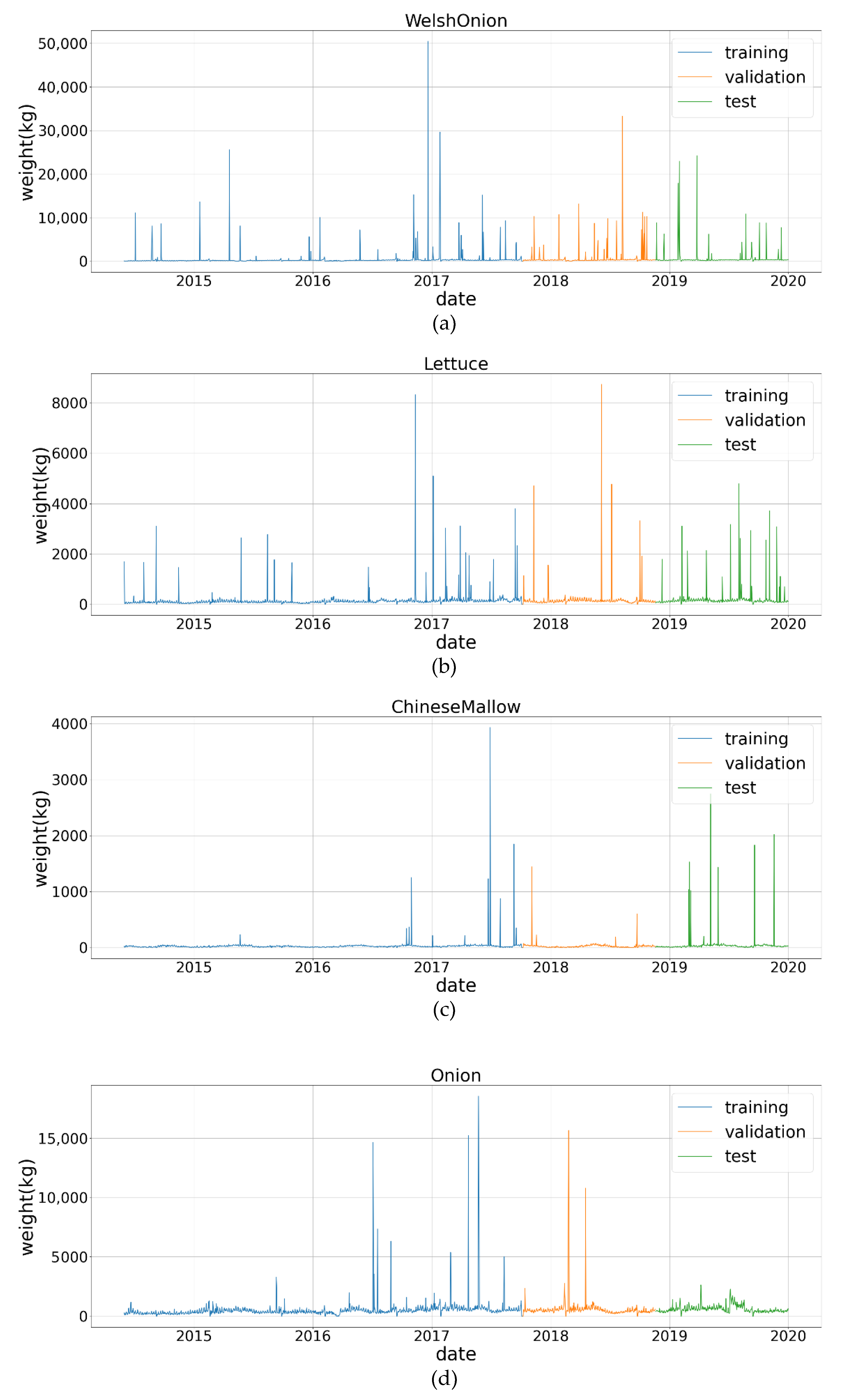
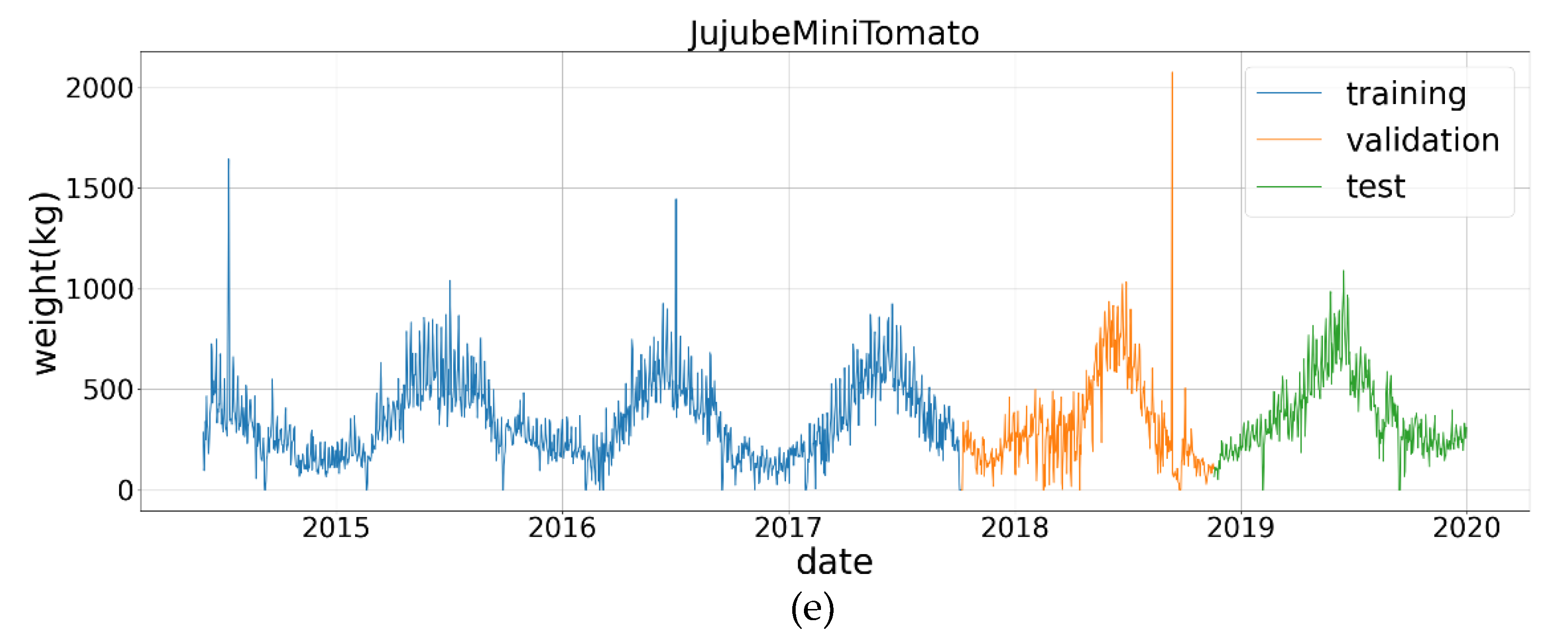
3.1. Data

3.1.1. Data Collection and Observations

The dataset used in the proposed method was extracted from a database of the sales volume of about 3000 items sold in the POS (point of sale) system of a local food retail store in Wanju, South Korea. The time-series data of five items (WelshOnion, Lettuce, ChineseMallow, Onion, and JujubeMiniTomato) that showed the least number of missing dates were chosen. The sales period for the five items was from June 2014 to December 2019, so each sales time-step was around T = 2000 days or more, where T is the total number of time-steps. Table 1 presents the sales periods and the sales days of the five items.
The difference between the number of days (T) and the sales days in Table 1 is due to the fact that the data contains missing values for various reasons, such as holidays at the Wanju local food retail store and a lack of supply of certain products. Figure 1 shows the sales volume data of the five items.
Figure 2 shows the distribution of the values in the dataset for the five items. We noticed the presence of outliers in Figure 2. Outliers result from mistakes in sales volume input, such as numerical unit errors or decimal point notation errors in sales volume.
Figure 3 shows the correlation between each pair of the five items, and all correlations show weak relationships. The top-two most correlated pairs are Onion–Lettuce (0.36) and JujubeMiniTomato–ChineseMallow (0.35), while the least correlated pair is the JujubeMiniTomato–WelshOnion (0.00011). Figure 4 shows the average sales volumes by day, month, and quarter of Lettuce sales data from 1 June 2014 to 31 December 2019. Figure 4a shows that the average sales volume is the highest on Saturday, followed, in order, by Sunday and Friday. In Figure 4b, it can be seen that average sales are highest in March, followed, in order, by April and August. Figure 4c shows that average sales are in descending order of the first, third, second, and fourth quarters. Average sales in the second and third quarters are similar. As it shows a high degree of seasonality, embedding the seasonality information in the prediction models as weekly, monthly, and quarterly features is expected to improve prediction accuracy.

3.1.2. Data Preprocessing

As shown in Figure 1 and Figure 2, there are outliers and missing values in the data. The data is processed using the z-score with interpolation methods. In statistics, the z-score is the number of standard deviations by which the value of a raw score (i.e., an observed value or data point) is above or below the mean value of what is being observed or measured. Raw scores above the mean have positive standard scores, while those below the mean have negative standard scores. The following equation shows the z-score equation, where μ and σ respectively represent the mean and the standard deviation.
z = x μ σ  
We removed the outliers using the z-score method. After converting the data into z-scores, data points outside the range of 95% of the z-scores were removed as outliers. In the top plot of Figure 5, the blue line represents the raw data, and the orange line represents the data after removing outliers from the raw data. The bottom plot in Figure 5 shows the results of the interpolation of missing values (blue lines); the interpolated part is also enlarged and shown. The enlarged plot shows that the blue line is interpolated to an orange color. As presented in Table 1, there is a missing value in the raw data. Therefore, we interpolate the missing values according to the time index of the time-series data.

3.2. Forecasting Models

We used the most popular models (SARIMA, Prophet, LSTM, and the proposed SLSTM) in our experiment. Their features and implementation specifications are summarized as follows.

3.2.1. AutoArima

The SARIMA model is one of the most popular models that incorporate seasonality into time series forecasting [7,8,9]. It has a limitation—the user must select a proper model using autocorrelation function (ACF) and partial autocorrelation function (PACF) plots, as well as calculate the Akaike information criterion (AIC) or the Bayesian information criterion (BIC). To resolve this problem, the auto_arima method was developed, which automatically selects an optimal model [31]. In our implementation, we used the auto_arima function provided by the Python pmdarima library.
The auto_arima function fits the best ARIMA model to a time series according to a given information criterion (either AIC, BIC, or the Hannan–Quinn information criterion (HQIC)). The function performs a search (either stepwise or parallelized) for the possible model and the seasonal orders within the constraints provided, then selects the parameters that minimize the given metric. The auto_arima function itself operates a bit like a grid search, as it tries various sets of p and q (also P and Q for seasonal models) parameters, then selects the model that minimizes AIC or BIC. To select the differencing terms, the auto_arima function uses tests of stationarity (such as an augmented Dickey–Fuller test) and seasonality (such as the Canova Hansen test) for seasonal models [31].

3.2.2. Prophet

The Prophet model has an advantage—the parameters are interpretable so that the analyst can intuitively adjust them with domain knowledge of the time series. Tools that help analysts use their expertise effectively enable the reliable and practical forecasting of business time series [22]. The Prophet model is a procedure for forecasting time series data based on an additive model, where nonlinear trends are fit with yearly, weekly, and daily seasonality, plus holiday effects. We use the decomposable time series model outlined by Harvey and Peters [32], with three main model components: trend, seasonality, and holidays. They are combined in Equation (2).
y ( t ) = g ( t ) + s ( t ) + h ( t ) +   ϵ t
Here, g ( t ) is the trend function that models nonperiodic changes in the value of the time series, s ( t ) represents periodic changes (e.g., weekly and yearly seasonality), and h ( t ) represents the effects of holidays that occur in potentially irregular schedules over one or more days. The error term ϵ t represents any idiosyncratic changes that are not accommodated by the model; later, we will make a parametric assumption that ϵ t is normally distributed [22]. The Prophet model has various parameters related to g ( t ) , s ( t ) , and h ( t ) that can be set by the user. It also has parameters such as saturating forecasts to control the upper and lower limits of forecast values, trend changepoints to change trend pointers in the data, seasonality to directly create seasonal attributes and scale the seasons, holiday effects to set holidays and special events, regressors to add additional effects, multiplicative seasonality to apply to models with progressively increasing seasonality, and uncertainty intervals to indicate the range of uncertainty in the predicted values. The user can set these parameters to improve forecasting performance. By default, the Prophet model will automatically detect changepoints and will allow the trend to adapt appropriately. However, we can use a few input arguments to have more control over this process. In our experiment, we increased the input argument change_point_scale above the default value because of the underfit problem. We also used holidays as holiday effects.

3.2.3. Long Short-Term Memory

LSTM is an advanced architecture of RNN. LSTM has a long-range dependency that makes it more accurate than conventional RNNs. The basic structure of LSTM is considered to be a memory cell for remembering and explicitly propagating unit outputs in different time steps. The memory cell of LSTM uses cell states to remember the information of temporal contexts. It also has a forget gate, an input gate, and an output gate to control information flow between different time steps. The mathematical challenge associated with learning the long-term dependencies in the structure of recurrent neural networks is called the vanishing gradient problem. As the length of the input sequence increases, it becomes harder to capture the influence of the earliest stages, and the gradients to the first few input points vanish and become equal to zero. The LSTM model, which consists of a forget gate, an input gate, and an output gate, compensates for the disadvantages of RNN. The structure of the LSTM network is shown in Figure 6.
Activation functions that are commonly used in the LSTM network are sigmoid and hyperbolic tangent [12,24]. These activation functions of LSTM are calculated for forget gate f t , input gate i t , output gate o t , candidate vector c t , cell state c t , and hidden state h t using the following formulae, respectively:
f t =   σ ( w x f x t +   w h f h t 1 +   b f ) i t =   σ ( w x i +   w h i h t 1 +   b i ) c t =   t a n h ( w x c x t +   w h c h t 1 +   b c ) o t =   σ ( w x o x t +   w h o h t 1 +   b o ) c t =   f t * c t 1 +   i t *   c t h t =   o t * t a n h ( c t )
In the above equations, w x f , w x i , w x c , and w x o , used with x t , are, and w h f , w h i , w h c , and w h o , used with h t 1 , are the weight of each gate. The operator * means the element-wise multiplication. In addition, b f , b i , b c , and b o are the biases used at each gate. The prediction problem using LSTM creates input data in a pattern of a constant length, as shown in Figure 7. The input of the LSTM model is controlled by the window size ( w ) and the horizon factor ( h ). The window size indicates the number of consecutive time-steps that are used in feature vector X, while the horizon factor represents how far ahead predictions are being made. In Figure 7, w = 3 and h = 2.
The LSTM model in this section and the SLSTM model in the following section were trained using a Python package called Keras on top of the Tensorflow backend. For a fair comparison, the same hyperparameters were used for LSTM and SLSTM in the experiment. The detailed specification of the hyperparameter setting is given in Section 4.

3.2.4. Seasonal Long Short-Term Memory

The essential part of the proposed seasonal long short-term memory (SLSTM) model is how to explicitly input the weekly and monthly information in the input layer of LSTM. Due to the flexibility of LSTM architecture, this task is easy to accomplish. In our method, we extend the time series data by adding the seasonal information about week, month, and quarter. The weekly, monthly, and quarterly information are regarded as features, and those features are entered into the SLSTM network model individually or in combination. In the following formula, S represents weekly ( S w ), monthly ( S m ), and quarterly ( S q ) features or consists of their combination. Seasonal features are added in the form of one-hot codes, as follows:
S i = ( S i w , S i m , S i q , S i w m , S i m q , S i w q , S i w m q ) S i w   =   ( Monday ,   Tuesday ,   Wednesday ,   Thursday ,   Friday ,   Saturday ,   Sunday ) =   ( 0 ,   1 ,   0 ,   0 ,   0 ,   0 ,   0 ) ,   when   i   is   Tuesday . S i m   =   ( January ,   February ,   March ,   April ,   May ,   June ,   July ,   August ,   September ,   October ,   November ,   December ) =   ( 0 ,   0 ,   1 ,   0 ,   0 ,   0 ,   0 ,   0 ,   0 ,   0 ,   0 ,   0 ) ,   when   i   is   March . S i q   =   ( the   first   quarter ,   the   sec ond   quarter ,   the   third   quarter ,   the   fourth   quarter ) =   ( 0 ,   1 ,   0 ,   0 ,   0 ) ,   when   i   is   the first quarter . S i w m   =   S i w   +   S i m ,   S i m q   =   S i m   +   S i q ,   S i w q   =   S i w   +   S i q ,   S i w m q   =   S i w   +   S i m   +   S i q ,   where   +   indicates   the   concatenation   of   two   one - hot   codes .
The input data of the network is sampled by concatenating S i w and x i . If x i is Tuesday, it is sampled in the form ( x i , 0, 1, 0, 0, 0, 0, 0). Figure 8 shows the weekly features individually entered into the SLSTM network.

4. Experimental Results and Discussions

4.1. Experimental Environments

In the LSTM and SLSTM models, the sales volume datasets were split into three subsets, with the first 60% of the data considered as the training set, the next 20% as the validation set, and the most recent 20% as the test set. The validation set was used to estimate the hyperparameters of the individual models. We found a reasonable hyperparameter setting using the validation set for the LSTM model and used the same values for the SLSTM model. Our setting was that the number of hidden nodes is 128, the learning rate is le-04, the optimizer is Adam, the loss function is mean squared error (MSE), the number of epochs is 500, and the batch size is 1. In the auto_arima and Prophet models, the dataset was split into two subsets, with the first 80% used as the training set and the remaining 20% as the test set.
The forecasting performances were evaluated in terms of three error measures: mean absolute error (MAE), root mean squared error (RMSE), and normalization mean absolute error (NMAE). These measures are defined as follows in Equation (4), where y i and p i are the true value and predicted value, respectively, and n is the number of samples in the test set.
MAE :   1 n i = 1 n | y i t i |   RMSE :   1 n i = 1 n ( y i t i ) 2   NMAE :   1 n i = 1 n | y i t i | t i  
The measures can assume values greater than or equal to 0, where lower values are considered to be better. MAE expresses the absolute error, so it is easy to understand. RMSE assigns high penalties to large errors since the prediction errors are squared. NMAE is advantageous because it has the same scale across different products. For example, for the product with (1100,1000) for y and p, the NMAE is |1100 − 1000|/1000 = 0.1. For another product with (110,100), the NMAE is |110 − 100|/100 = 0.1. In terms of NMAE, these two products, with different scales, have the same error, 10%; by contrast, the MAE differs substantially from |1100 − 1000| = 100 to |110 − 100| = 10.
The experiment was performed on a computer equipped with an Intel(R)Xeon(R) Gold 6126 CPU (2.60 GHz) and an NVIDIA GeForce RTX 2080 Ti GPU.

4.2. Performance Comparisons

We illustrate the predictions by auto_arima, Prophet, LSTM, and SLSTM models using the lettuce data in Figure 9. The data in Figure 9 is the same as the test part (last 20%) of the data at the bottom of Figure 5. The predictions of the auto_arima model in Figure 9a reveals a large mismatch to the ground truth data. The predictions of the Prophet model in Figure 9b follow the trend of the ground truth, with a noticeable gap. The gap of the Prophet model increases after time-step 150. The Prophet model predicted smaller values than the ground truth, leading to lower accuracies. Compared to Prophet, LSTM’s predictions in Figure 9c and SLSTM’s predictions in Figure 9d follow the trend of the ground truth more accurately. These observations explain the superior accuracies of LSTM and SLSTM to auto_arima and Prophet.
Our main concern is for the comparison of LSTM and SLSTM. In the ground truth data in Figure 9, small and large peaks and drops in sales volume appear in many time steps. Looking carefully at the drops below 100, SLSTM predicts values that are much closer to the ground truth than LSTM. The same phenomena can be observed at the peaks reaching between 200 and 300. The same effect is noticed at almost every peak and drop. The effect explains the reason why SLSTM is superior to LSTM. For the large peaks appearing near time-steps 170, 210, 280, and 310, no model managed a close prediction.
The performance of the proposed SLSTM model was quantitatively compared with those of auto_arima, Prophet, and LSTM in terms of three performance metrics (MAE, RMSE, and NMAE). In Table 2, sw, sm, sq, swm, smq, swq, and swmq represent the seasonal components, namely, the weeks, months, and quarters, as well as their combinations. The sales volumes of five items (WelshOnion (WO), Lettuce, ChineseMallow (CM), Onion, and JujubeMiniTomato (JMT)) were used in our experiment.
Overall, SLSTM shows the least error. As an example, the NMAE of SLSTM is below 0.20, while LSTM and Prophet show 0.26 and 0.39, respectively. The Prophet model is inferior to auto_arima, except for JMT and Onion. The LSTM model is better than Prophet, except for Onion.
The SLSTM model compared the different combinations of seasonality. We emphasize the best case by using bold typeface in Table 2. The seasonality factors sw, swm, swq produced good accuracies. Among them, swm (combination of week and month) seasonality shows the best accuracy.

4.3. Discussion

Most of the time-series data coming from a variety of application fields are difficult to use to forecast the future. The less stable patterns the data has, the more difficult it is to forecast. The data coming from agricultural areas are known to be the most fluctuating data due to various perturbation factors such as weather, local and global policies, and societal events. These uncertainties make the prediction of agroproduct sales volumes difficult [1]. The sales volume data from a local food shop used in our experiments also reveal high fluctuation, as shown in Figure 1. The large peaks and sudden drops appear in many time steps. All of the four models could not predict the large peaks and sudden drops, as shown in Figure 9. Even human experts cannot predict the sudden changes without prior information on what incurs those changes. To overcome the limitation of the prediction models, we should inject further information from news and SNS into the prediction model. This issue has seldom been studied in the machine learning community, leaving it as a challenging research subject.
As the weekly, monthly, and quarterly seasonality of every time step is known in advance, we attempted to explicitly inject the seasonality information into the neural network LSTM model. As expected, this attempt improved the prediction accuracies significantly, as shown in Table 2. The combination of the weekly and monthly information showed the best accuracy in our experiment. The standard LSTM model has the ability to model seasonality. However, its ability is limited to discovering the seasonal patterns in the data and representing the implicit patterns in the model. We argue that the explicit injection of seasonal information improves the accuracy significantly.
In [4], a new metric measuring the conservation of statistical characteristics was proposed. The metric reflects how well the model predictions conserve the statistical trends of the original data. The author of the paper insisted that this metric is important to evaluating a forecasting model thoroughly since the accuracy metric evaluates every time step individually. This new metric can be applied to any time-series data. Its application to our data is regarded as future work.

5. Conclusions

People have long been interested in predicting future events. However, predicting future events is difficult, and various studies are being conducted to identify methods for more accurate predictions. In this paper, we propose the SLSTM method, which is a system for predicting the sales of agricultural products in order to stabilize supply and demand. SLSTM with intensified seasonality shows a low forecasting error rate and NMAE in performance comparison experiments with auto_arima, Prophet, and standard LSTM models. Important future work should include climate and weather information in the model because agricultural forecasting is heavily affected by climate and weather. Another future work is related to applying recently proposed Transformer models such as BERT and GPT.

Author Contributions

T.-W.Y. wrote and implemented the algorithm. I.-S.O. supervised and supported this study. All authors have read and agreed to the published version of the manuscript.

Funding

This research was funded by the Cross-Ministerial Collaboration Cloud Innovation Case Creation (All@Cloud 2019) Project through the National IT Industry Promotion Agency (NIPA) (No. A0301-19-1003).

Conflicts of Interest

The authors declare no conflict of interest.

References

  1. Huchet-Bourdon, M. Agricultural Commodity Price Volatility: An Overview (No. 52); OECD Food, Agriculture and Fisheries Papers; OECD Publishing: Paris, France, 2011. [Google Scholar] [CrossRef]
  2. Kamilaris, A.; Kartakoullis, A.; Prenafeta-Boldu, F.X. A review on the practice of big data analysis in agriculture. Comput. Electron. Agric. 2017, 143, 23–37. [Google Scholar] [CrossRef]
  3. Kamilaris, A.; Prenafeta-Boldu, F.X. Deep learning in agriculture: A survey. Comput. Electron. Agric. 2018, 147, 70–90. [Google Scholar] [CrossRef] [Green Version]
  4. Kurumatani, K. Time series forecasting of agricultural product prices based on recurrent neural networks and its evaluation method. SN Appl. Sci. 2020, 2, 1434. [Google Scholar] [CrossRef]
  5. Wang, J.; Wang, Z.; Li, X.; Zhou, H. Artificial bee colony-based combination approach to forecasting agricultural commodity prices. Int. J. Forecast. 2019. [Google Scholar] [CrossRef]
  6. Ahmad, A.; Javaid, N.; Mateen, A.; Awais, M.; Khan, Z.A. Short-term load forecasting in smart grids: An intelligent modular approach. Energies 2019, 12, 164. [Google Scholar] [CrossRef] [Green Version]
  7. Raza, M.Q.; Khosravi, A. A review on artificial intelligence based load demand forecasting techniques for smart grid and buildings. Renew. Sustain. Energy Rev. 2015, 50, 1352–1372. [Google Scholar] [CrossRef]
  8. Dauta, M.A.M.; Hassana, M.Y.; Abdullaha, H.; Rahmana, H.A.; Abdullaha, M.P.; Hussina, F. Building electrical energy consumption forecasting analysis using conventional and artificial intelligence methods: A review. Renew. Sustain. Energy Rev. 2017, 70, 1108–1118. [Google Scholar] [CrossRef]
  9. Deb, C.; Zhang, F.; Yanga, J.; Lee, S.E.; Shah, K.W. A review on time series forecasting techniques for building energy consumption. Renew. Sustain. Energy Rev. 2017, 74, 902–924. [Google Scholar] [CrossRef]
  10. Gao, Y.; Fang, C.; Ruan, Y. A novel model for the prediction of long-term building energy demand: LSTM with Attention layer. IOP Conf. Ser. Earth Environ. Sci. 2019, 294, 012033. [Google Scholar] [CrossRef]
  11. Nguyen, H.V.; Naeem, M.A.; Wichitaksorn, N.; Pears, R. A smart system for short-term price prediction using time series models. Comput. Electr. Eng. 2019, 76, 339–352. [Google Scholar] [CrossRef]
  12. Poornima, S.; Pushpalatha, M. Prediction of rainfall using intensified LSTM based recurrent neural network with weighted linear units. Atmosphere 2019, 10, 668. [Google Scholar] [CrossRef] [Green Version]
  13. McNally, S.; Roche, J.; Caton, S. Predicting the price of bitcoin using machine learning. In Proceedings of the 26th Euromicro International Conference on Parallel, Distributed, and Network-Based Processing, Cambridge, UK,, 21–23 March 2018; pp. 339–343. [Google Scholar] [CrossRef] [Green Version]
  14. Vochozka, M.; Vrbka, J.; Suler, P. Bankruptcy or success? the effective prediction of a company’s financial development using LSTM. Sustainability 2020, 12, 7529. [Google Scholar] [CrossRef]
  15. Hao, Y.; Gao, Q. Predicting the Trend of Stock Market Index Using the Hybrid Neural Network Based on Multiple Time Scale Feature Learning. Appl. Sci. 2020, 10, 3961. [Google Scholar] [CrossRef]
  16. Mondal, P.; Shit, L.; Goswami, S. Study of effectiveness of time series modeling (ARIMA) in forecasting stock prices. Int. J. Comput. Sci. Eng. Appl. (IJCSEA) 2014, 4, 13–29. [Google Scholar] [CrossRef]
  17. Goodfellow, I.; Bengio, Y.; Courville, A. Deep Learning; The MIT Press: Cambridge, MA, USA, 2016. [Google Scholar]
  18. Chou, J.S.; Ngo, N.T. Time series analytics using sliding window metaheuristic optimization-based machine learning system for identifying building energy consumption patterns. Appl. Energy 2016, 177, 751–770. [Google Scholar] [CrossRef]
  19. Divina, F.; Torres, M.G.; Vela, F.A.G.; Noguera, J.L.V. A comparative study of time series forecasting methods for short term electric energy consumption prediction in smart buildings. Energies 2019, 12, 1934. [Google Scholar] [CrossRef] [Green Version]
  20. Ruekkasaem, L.; Sasananan, M. Forecasting agricultural products prices using time series methods for crop planning. Int. J. Mech. Eng. Technol. (IJMET) 2018, 9, 957–971. [Google Scholar]
  21. Box, G.E.P.; Jenkins, G.M. Time Series Analysis: Forecasting and Control; Holden Day: San Francisco, CA, USA, 1976. [Google Scholar]
  22. Taylor, S.J.; Letham, B. Forecasting at scale. Am. Stat. 2018, 72, 37–45. [Google Scholar] [CrossRef]
  23. Tran, N.; Nguyen, T.; Nguyen, B.M.; Nguyen, G. A multivariate fuzzy time series resource forecast model for clouds using LSTM and data correlation analysis. Procedia Comput. Sci. 2018, 126, 636–645. [Google Scholar] [CrossRef]
  24. Hochreiter, S.; Schmidhuber, J. Long short-term memory. Neural Comput. 1997, 9, 1735–1780. [Google Scholar] [CrossRef]
  25. Neil, D.; Pfeiffer, M.; Liu, S.C. Phased LSTM: Accelerating recurrent network training for long or event-based sequences. In Proceedings of the 30th Conference on Neural Information Processing Systems (NIPS 2016), Barcelona, Spain, 9 September 2016; pp. 3889–3897. [Google Scholar] [CrossRef]
  26. Hsu, D. Multi-period time series modeling with sparsity via Bayesian variational inference. arXiv 2018, arXiv:1707.00666v3. [Google Scholar]
  27. Khashei, M.; Bijari, M.; Ardali, G.A.R. Improvement of auto-regressive integrated moving average models using fuzzy logic and artificial neural networks (ANNs). Neurocomputing 2009, 72, 956–967. [Google Scholar] [CrossRef]
  28. Cenas, P.V. Forecast of agricultural crop price using time series and Kalman filter method. Asia Pac. J. Multidiscip. Res. 2017, 5, 15–21. [Google Scholar]
  29. Anggraeni, W.; Mahananto, F.; Sari, A.Q.; Zaini, Z.; Andri, K.B. Sumaryanto, Forecasting the price of Indonesia’s rice using Hybrid Artificial Neural Network and Autoregressive Integrated Moving Average (Hybrid NNs-ARIMAX) with exogenous variables. Procedia Comput. Sci. 2019, 161, 677–686. [Google Scholar] [CrossRef]
  30. Fang, Y.; Guan, B.; Wu, S.; Heravi, S. Optimal forecast combination based on ensemble empirical mode decomposition for agricultural commodity futures prices. J. Forecast. 2020, 39, 877–886. [Google Scholar] [CrossRef]
  31. Smith, T.G. Pmdarima: ARIMA Estimators for Python. 2017. Available online: http://www.alkaline-ml.com/pmdarima (accessed on 25 February 2020).
  32. Harvey, A.; Peters, S. Estimation procedures for structural time series models. J. Forecast. 1990, 9, 89–108. [Google Scholar] [CrossRef]
Figure 1. Sales volumes of five items (WelshOnion (a), Lettuce (b), ChineseMallow (c), Onion (d), and JujubeMiniTomato (e)). Note that the y-axis scale of each plot is different. The first 60% was used for the training subset (blue line), the next 20% was used for the validation subset (orange line), and the most recent 20% was used for the test subset (green line).
Applsci 10 08169 g001aApplsci 10 08169 g001b
Figure 2. Boxplot of sales volumes of five items (WelshOnion (WO), Lettuce (L), ChineseMallow (CM), Onion (O), and JujubeMiniTomato (JMT)).
Applsci 10 08169 g002
Figure 3. Correlation matrix among sales volumes of five items (WelshOnion (WO), Lettuce (L), ChineseMallow (CM), Onion (O), and JujubeMiniTomato (JMT)).
Applsci 10 08169 g003
Figure 4. Average sales of lettuce data by day, month, and quarter. (a) Average sales by day of week, (b) average sales by month, and (c) average by quarter.
Applsci 10 08169 g004aApplsci 10 08169 g004b
Figure 5. In the (top) plot, the blue and orange lines are the raw data and the data after removing outliers, respectively. The (bottom) plot shows that the missing values (blue line) of the orange line are interpolated; a part of the bottom plot is also enlarged and shown.
Applsci 10 08169 g005
Figure 6. Schematic representation of long short-term memory (LSTM) model.
Applsci 10 08169 g006
Figure 7. LSTM input data sample creation. (a) Data sampling for LSTM input ( w = 3, h = 2). (b) Representation of feature vector X and label Y.
Applsci 10 08169 g007
Figure 8. Seasonal long short-term memory (SLSTM) input data creation. (a) Data sampling with seasonality extension ( w = 3 , h = 2 S i =   S i w ). (b) Representation of feature vector X and label Y.
Applsci 10 08169 g008
Figure 9. The result predicted by auto_arima (a), Prophet (b), LSTM (c), and SLSTM (d) models (only using sw) with lettuce data.
Applsci 10 08169 g009
Table 1. The sales periods and the sales dates of the five items.
No.ItemSales DaysPeriodT
1WelshOnion20141 June 2014~31 December 20192040
2Lettuce20141 June 2014~31 December 20192040
3ChineseMallow20121 June 2014~31 December 20192040
4Onion20091 June 2014~31 December 20192040
5JujubeMiniTomato20111 June 2014~31 December 20192040
Table 2. The experimental results for WelshOnion (WO), Lettuce, ChineseMallow (CM), Onion, and JujubeMiniTomato (JMT).
ItemMetricAuto_ArimaProphetLSTMSLSTM
swsmsqswmsmqswqswmq
WOMAE122.87139.83121.2114.47113.9111.45111.37113.96111.75113.67
RMSE430.72438.1428.6402.59402.22399.56400.76402.22400.62401.67
NMAE0.320.330.260.190.190.190.180.190.180.19
LettuceMAE50.1849.045.7333.0638.1838.9832.8336.9934.0633.35
RMSE88.9987.183.4977.5580.2280.5977.8879.9278.9477.30
NMAE0.280.310.290.190.240.240.190.230.200.20
CMMAE7.948.37.57.317.777.747.447.827.438.27
RMSE12.9513.412.812.7913.1112.9513.0412.9912.7113.85
NMAE0.350.370.350.270.30.30.280.290.290.3
OnionMAE233.47233.6237.6208.99225.36235.73196.55212.95190.74192.3
RMSE373.37358.8376.1347.8362.86374.16331.97348.26324.47325.64
NMAE0.290.290.310.250.280.290.250.270.240.25
JMTMAE114.5189.278.376.5774.2376.0965.3275.6274.8974.32
RMSE156.06105.8101.8100.8196.09100.0585.7598.799.6996.53
NMAE0.340.270.260.230.200.230.170.200.190.19
Publisher’s Note: MDPI stays neutral with regard to jurisdictional claims in published maps and institutional affiliations.

