Article

Developing a New Hourly Forest Fire Risk Index Based on Catboost in South Korea

1
Department of Urban & Environmental Engineering, Ulsan National Institute of Science and Technology, Ulsan 44919, Korea
2
Division of Forest Disaster Management, Korea Forest Research Institute, Seoul 02455, Korea
*
Author to whom correspondence should be addressed.
Appl. Sci. 2020, 10(22), 8213; https://doi.org/10.3390/app10228213
Submission received: 27 October 2020 / Revised: 12 November 2020 / Accepted: 17 November 2020 / Published: 19 November 2020
(This article belongs to the Special Issue Advanced Remote Sensing Technologies for Disaster Monitoring)

Abstract

:
Forest fires can cause enormous damage, such as deforestation and environmental pollution, even with a single occurrence. It takes a lot of effort and long time to restore areas damaged by wildfires. Therefore, it is crucial to know the forest fire risk of a region to appropriately prepare and respond to such disastrous events. The purpose of this study is to develop an hourly forest fire risk index (HFRI) with 1 km spatial resolution using accessibility, fuel, time, and weather factors based on Catboost machine learning over South Korea. HFRI was calculated through an ensemble model that combined an integrated model using all factors and a meteorological model using weather factors only. To confirm the generalized performance of the proposed model, all forest fires that occurred from 2014 to 2019 were validated using the receiver operating characteristic (ROC) curves and the area under the ROC curve (AUC) values through one-year-out cross-validation. The AUC value of HFRI ensemble model was 0.8434, higher than the meteorological model. HFRI was compared with the modified version of Fine Fuel Moisture Code (FFMC) used in the Canadian Forest Fire Danger Rating Systems and Daily Weather Index (DWI), South Korea’s current forest fire risk index. When compared to DWI and the revised FFMC, HFRI enabled a more spatially detailed and seasonally stable forest fire risk simulation. In addition, the feature contribution to the forest fire risk prediction was analyzed through the Shapley Additive exPlanations (SHAP) value of Catboost. The contributing variables were in the order of relative humidity, elevation, road density, and population density. It was confirmed that the accessibility factors played very important roles in forest fire risk modeling where most forest fires were caused by anthropogenic factors. The interaction between the variables was also examined.

1. Introduction

Forest fires have a profound impact on ecological processes on the Earth, such as deforestation, habitat destruction, and loss of soil nutrients, as well as the environmental, economic, and social sectors [1,2,3]. It takes a long time and significant effort to restore areas with forest fires to their previous state. Therefore, it is necessary to make efforts to reduce the damage caused by forest fires. One such effort is to identify areas with high forest fire risk in advance to establish proper mitigation and response plans from a management perspective.
In recent years, many studies have also tried to predict where a forest fire is likely to occur [1,4,5,6]. Anthropogenic, topographic, meteorological, and fuel factors are mainly used to calculate fire risk [7,8,9]. The anthropogenic factors, such as distance from roads, distance from rivers, and urban areas, and topographic factors, such as elevation and slope, have been used for accessibility consideration [10,11]. As meteorological data, temperature, relative humidity, precipitation, and wind speed have been mainly used to consider dry weather conditions prone to fires. These meteorological variables have been typically extracted by interpolating station values or from numerical model data [7,12]. Some studies usually utilized satellite-derived indices to extract fire-prone dry fuel or weather conditions to explain the relationship between input factors and forest fires. However, there are limitations due to cloud contamination and coarse spatial or temporal resolution when using optical satellite sensor systems [4].
To predict forest fire susceptibility and risk, a lot of efforts have been made worldwide. The Canadian Forestry Service has developed the Canadian Forest Fire Weather Index (CFWI) and has been officially conducting forest fire risk forecasting since 1970. CFWI has been widely studied for its feasibility in many countries including Australia, the United Kingdom, Greece, China, and South Korea [5,13,14,15,16,17]. The Met Office Fire Severity Index (MOSPI) forest fire risk forecasting system provided by the UK is also based on CFWI [18]. CFWI is a weather index that combines fine fuel moisture code (FFMC), duff moisture code (DMC), drought code (DC), initial spread index (ISI), and build up index (BUI) information obtained using weather information such as temperature, relative humidity, wind speed, and precipitation [19]. CFWI has complicated calculation processes and empirical standards (i.e., coefficients for formula), and thus may not fit well for other areas with different weather conditions, requiring additional careful calibration [20,21,22].
The Korea Forest Service’s National Forest Research Institute (NFRI) uses weather data—temperature, relative humidity, and wind speed—to calculate real-time Daily Weather Index (DWI) based on logistic regression [23]. NFRI provides DWI showing the degree of forest fire risk by administrative units. DWI is classified into four fire risk classes (low, moderate, high, and very high), providing real-time and 72-h forecasts at the 3-h interval [23,24]. DWI is mainly focused on weather factors without consideration of other accessibility or surface factors. Thus, it might not work well to predict the susceptibility of forest fires that frequently occur due to anthropogenic factors. In particular, the forest fires caused by anthropogenic factors such as incineration of paddy fields, waste incineration, and cigarettes exceed 70% according to historical data from 2010 to 2019 in South Korea. According to Kim et al. [25], human activities and accessibility in South Korea are closely related to the probability of forest fire occurrence. Thus, it is necessary to develop a forest fire risk monitoring model that considers not only weather conditions but also topographic and anthropogenic factors.
In order to simultaneously consider weather, fuel, topography, and anthropogenic factors, it is advantageous to use machine learning. In particular, machine learning has proved successful in applying a multitude of variables for predicting forest fire risk [8,9,26]. Main input variables to the forest fire risk prediction include satellite-derived vegetation indices, anthropogenic factors such as proximity to roads, meteorological factors such as temperature, and hydrological factors such as rainfall [26]. Many studies have modeled forest fire susceptibility based on the binary information with forest fire location or its surrounding areas as 1 and non-fire areas far from forest fires as 0. A variety of machine learning approaches including artificial neural networks, random forest (RF), support vector machines, generalized additive model, and boosted regression trees have been used for forest fire risk modeling [7,8,20,27].
However, many of the studies have used fixed parameters and focused on long-term (i.e., yearly, monthly) fire risk. Nowadays, studies on dynamic models focusing on short-term (i.e., daily, sub-daily) fire risk are becoming active [5]. Since forest fire risk has its diurnal cycle, it is necessary to derive a forest fire risk index at very short time scale (i.e., every hour) to provide practical information for decision making on forest fire management. Thus, there is still room for improvement such as providing forest fire susceptibility and risk hourly or sub-hourly. So far, machine learning-based forest fire susceptibility studies have focused on a few large forest fire cases or are not updated with time (not hourly) [5,28]. When an approach is proposed for fire risk prediction, its transferability should be evaluated on both spatial and temporal domains.
Therefore, this study aims to propose a new hourly forest fire risk index (HFRI) at 1 km resolution over South Korea. Specifically, the measurable objectives of this research were to (1) develop a machine learning-based ensemble approach that combines two models with the topographic and anthropogenic factors as well as weather factors, (2) analyze the impact of each factor on HFRI, and (3) to evaluate the transferability of the proposed approach on a temporal domain. As mentioned above, forest fires in South Korea have mainly been caused by anthropogenic factors. Thus, the proposed HFRI that synergistically integrates weather, topographic, and anthropogenic factors is expected to better predict the forest fire risk in South Korea than other risk indices based solely on weather conditions such as DWI.

2. Study Area and Data
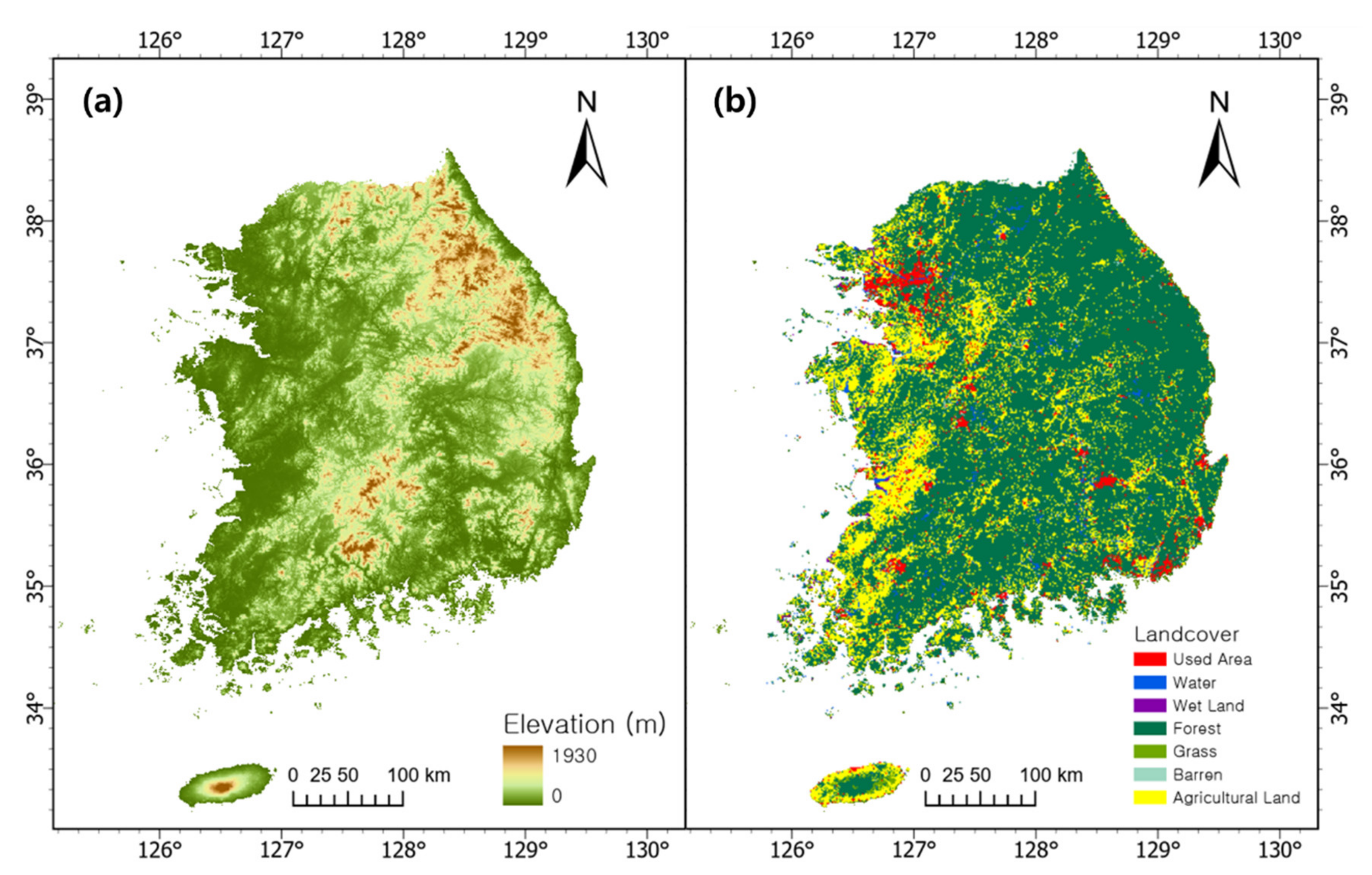
2.1. Study Area

The study area is South Korea where more than 70% of the land is forested areas (Figure 1). While the mean altitude is 448 m, the mean slope is 5.7°, which is about 2° steeper than the overall average of 3.9° in East Asia including Japan, the east part of Mongolia, and China [29]. Most forest fire cases have occurred in the spring season when the weather is dry and warm, and hikers frequently visit forested areas. On the other hand, the number of forest fire occurrences in summer is very low due to the highly concentrated precipitation and relatively high humidity. Among the forest fire events that occurred from 2010 to 2019, 58% occurred in spring, followed by winter (23%) [30]. The frequency and intensity of forest fires continue to increase as on-going climate change tends to increase extreme weather conditions [30].

2.2. Data

In this study, major weather factors, geographical data considering accessibility, fuel data, and time-related data related to the seasonal pattern of forest fires were used as input data to develop forest fire risk models. The input variables are summarized in Table 1.

2.2.1. Weather Data

The Digital Forecast is the weather forecast information provided by the Korea Meteorological Administration at 5 km resolution every 3 h based on the Unified Model Regional Data Assimilation and Prediction System numerical forecast model. It forecasts weather conditions hourly for the first two hours and with the three-hour interval after that up to two days (48 h). Digital Forecast provides basic meteorological products including temperature, precipitation, relative humidity, wind direction, and wind speed. The real-time Digital Forecast data are post-processed by Observation Data Analysis Module (ODAM) utilizing the in-situ observations [33]. In this study, the ODAM data were used for forest fire risk modeling. Among the products from Digital Forecast, relative humidity, temperature, and wind speed that affect forest fire occurrences were used in this study [1,34].

2.2.2. Geographical Data

The elevation from the ALOS World 3D 30 m (AW3D30) provides height information above the sea level globally at 1 arcsecond (approximately 30 m) resolution. It was released in May 2016 and updated in April 2020 by the Japan Aerospace Exploration Agency. It was constructed using the Panchromatic Remote-sensing Instrument for Stereo Mapping boarded on the Advanced Land Observing Satellite [35]. Studies have shown that AW3D30 has a better skill core than Shuttle Radar Topography Mission Digital Elevation Model (DEM) or Advanced Spaceborne Thermal Emission and Reflection Radiometer DEM in the Philippines and Mexico that have rugged mountains at high altitudes [35,36,37]. In particular, AW3D30 showed the most stable results among the three models even on the high altitude and dense vegetation. The elevation data were used as input considering accessibility because areas at the high altitude are less accessible by people, reducing the chance of forest fire occurrences.
The population density was derived from the Gridded Population of the World, Version 4, and Revision 11 data provided by the Society Economic Data and Applications Center [38]. The population density is provided as raster data at multiple spatial scales from 30 arcseconds to 60 arcminutes all over the world. As it is provided every five years from 2000, this study used 30 arcseconds (~1 km) data generated in 2015. The road density was calculated using the global road dataset provided by the Global Roads Inventory Project [39]. It contains five types of roads: highways, primary roads, secondary roads, tertiary roads, and local roads [40]. In this study, road density was calculated from the GRIP vector data (all road types) through the line density function in the ArcGIS 10.4 program. The population and the road densities were also used as factors to indirectly consider accessibility.

2.2.3. Fuel Data

The forest density was calculated using the forest type data provided by the Korea Forest Service’s Forest Geospatial Information System [41]. The forest type map has been produced every five years using aerial photography and field observations at two spatial scales: 1:5000 and 1:25,000 scale. The forest type map contains information on forest type, diameter-at-breast class, age class, and density. This study used the density data at the 1:25,000 scale. Forest density is classified into three categories, divided into forest stands with a crown area of 50 percent or less, those with 51 to 70 percent, and those with 71 percent or more. A larger value means a higher density.

2.2.4. Time-Related Data

In the study area, forest fire occurrences were concentrated in spring and winter while they were not frequent in summer and fall. Therefore, day of the year (DOY) was used as a variable to consider the seasonality of forest fires. DOY has been used as a variable after converting through sine or cosine functions to consider seasonality in many studies [42,43]. In this study, the sine function was applied to DOY, which generated a value between −1 (winter) and 1 (summer) with one year period.

2.2.5. In Situ Observation Data

The in-situ forest fire observation data provided by the Korea Forest Service were used for training and validation of the proposed models. The observation data contain the time from the start of a forest fire to the extinguishment, as well as information on the location, area, and cause of the forest fire. In this study, forest fire cases occurred from 2014 to 2019 were used, resulting in a total of 3118 cases. It should be noted that only eight of these cases caused large damaged areas more than 100 ha, while most resulted in damaged areas less than 5 ha.

3. Methods

The process flow of this study consists of three main parts: data preprocessing, machine learning modeling, and model validation (Figure 2). The input variables were first preprocessed to have the same spatial extent and resolution. Multicollinearity of the variables was then tested using the variance inflation factor (VIF). Monthly forest fire density through the stratified sampling was finally generated in the preprocessing stage. An ensemble model combining two machine learning models with different input variables was developed in the modeling part. The ensemble model was cross-year validated (One-year-out cross-validation) and further compared to the existing forest fire risk indices. One-year-out cross-validation refers to excluding one-year data for validation and training the model with the remaining five-year data. By repeating this process for each year (i.e., six times), all six years were cross-validated. The spatial distribution of the hourly forest fire risk index was qualitatively evaluated as well.

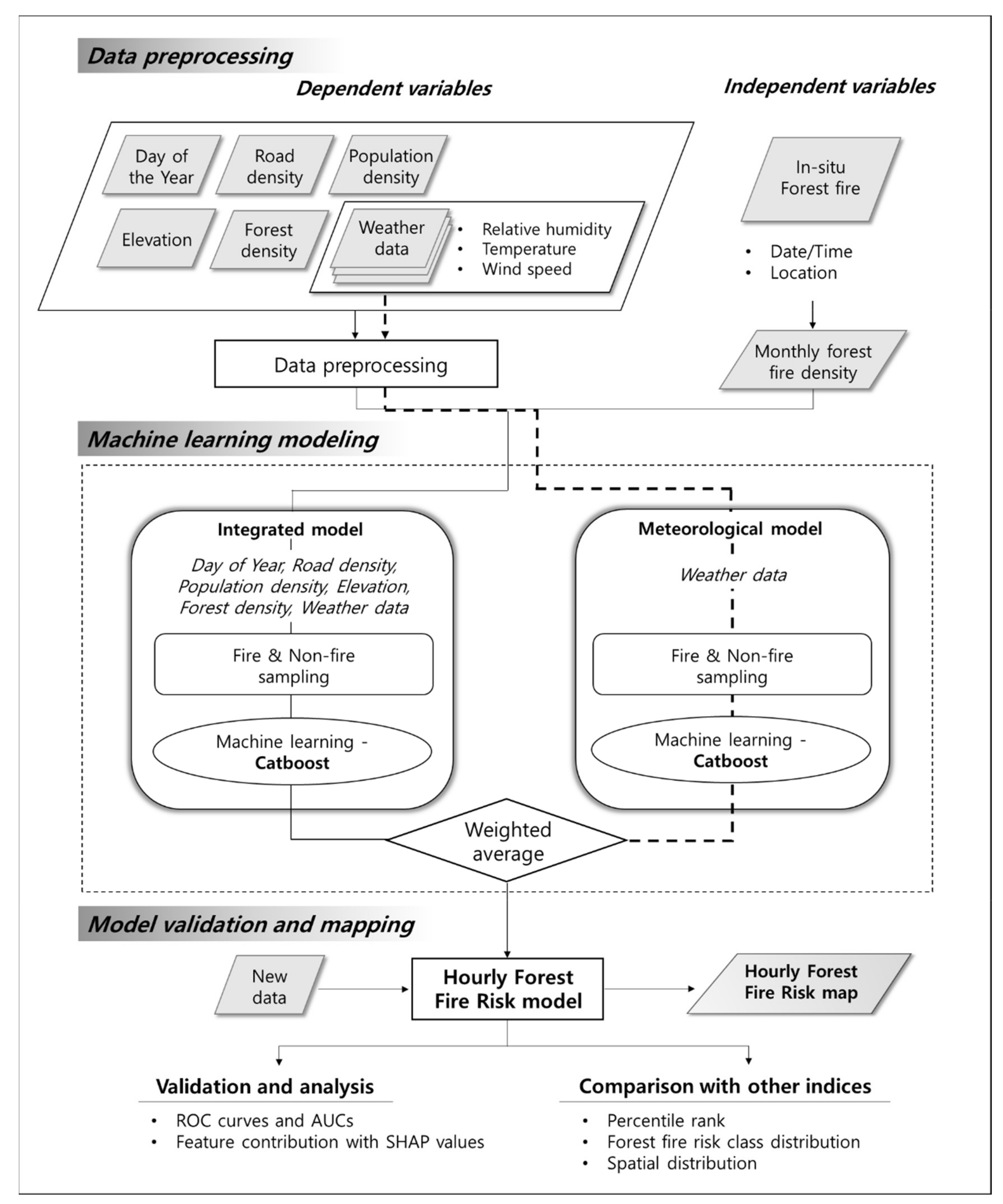
3.1. Data Preprocessing

Since input data have different spatial scales, all data were aggregated using an average function or resampled using the nearest neighbor to 1 km: Among the data used in this study, Roaddens, Popdens, elevation, and DN with less than 1 km spatial resolution were aggregated to the target resolution of 1 km using an average function. The smoothing effect caused by upscaling the original fine resolution data was negligible to the model performance (Supplementary Figure S1). The weather data at 5 km spatial resolution were simply downscaled to 1 km so that all 25 pixels in a 5-km grid have the same value. The VIF test was used to examine the multicollinearity between the input variables. VIF values > 10 generally indicate high multicollinearity between the variables, so the value of 10 is often used as a threshold for the VIF test [7,44]. In this study, all VIF values were below 10, so all input variables were used to develop the models.
Since this study was to develop a forest fire risk index, we approached it as a regression problem targeting forest fire risk rather than the binary classification of forest fire and non-fires. However, since in-situ data were provided only for forest fire occurrences, reference data for low forest fire risk were extracted in the areas where fires did not occur. To extract non-fire pixels (i.e., very low fire risk), the statistics of historical data were used. Monthly forest fire density was calculated using data of the past five years for each sampling year, resulting in a normalized value ranging from 0 to 1. For example, to extract non-fire samples in January 2015, the monthly forest fire density was calculated using January data from 2010 to 2014. If there were many fire occurrences in the surrounding areas of a location in the past 5 years, the location would have a high density. The density was then divided into four classes (25% each) using the percentiles for stratified sampling (i.e., non-fire samples were evenly extracted for each class). Note that the monthly forest fire density was only used as a supporting material to allocate the dependent variable value of non-fire samples and was not itself used as a dependent variable. The pixels with the high-density class (the top 25%) were excluded for extracting non-fire samples, while the pixels with the lower density classes had values from 0 to 0.2 (Table 2). The reason for assigning different values instead of 0 value to all non-fire pixels is to ensure the reliability of the non-fire pixel selection in the consideration of the forest fire pattern in recent years. In many studies on wildfire susceptibility, fires and non-fires were designated as 1 and 0, respectively, which often resulted in bimodal output (i.e., very high close to 1 and very low close to 0) with limited areas that have moderate susceptibility (e.g., 0.5–0.6) [9,45]. If no forest fire has occurred at a region in the past years, the forest fire risk for the region might be statistically low, so it is desirable to allocate it to zero. However, the forest fire risk of the region might not be low if the region suffered from forest fires in the past considering the causes of the fires. Thus, we assigned low values to some non-fire samples with moderate forest fire density. The values of 0.1 and 0.2 were empirically determined by testing multiple combinations. It should be noted that the proposed model was designed to predict forest fire risk, not to detect forest fires themselves.

3.2. Machine Learning Modeling

An ensemble model was proposed in this study, combining two machine learning models with different input variables. The reason for adopting the ensemble approach is to complement the different characteristics of two types of input variables: static variables and dynamic weather variables. As forest fires generally occur due to anthropogenic factors in South Korea, static input variables such as Popdens and Roaddens often have a relatively higher influence on the model than other dynamic variables (Supplementary Figure S2), which tends to result in high risk around urban areas all the time in the model results when using all variables (hereinafter, the integrated model). To mitigate the problem, the meteorological model based only on weather input variables was developed to show the seasonal and diurnal changes of forest fire risk. These two models were linearly combined through the weighted averaging approach to produce the final HFRI. The empirically determined optimum weighting ratio was 8:2 (i.e., integrated model: meteorological model).
The pixels of in-situ forest fire observations within the fire duration up to eight hours were assigned with a value of “1” showing the highest fire risk. Most forest fires occurred in the study area were extinguished within 8 h, except for a few very large (more than 100 ha damaged area) fires. In addition, even if a forest fire has continued over 8 h, it is difficult to determine whether the situation at that time is really a high forest fire risk. It should be noted that the model was targeting forest fire risk, not fire itself. Therefore, we used eight hours as a threshold when selecting training samples to avoid any impact from fire extinguishing work. Non-fire samples representing low fire risk were randomly extracted only at the time that forest fires have occurred in the forest areas except those within 5 km from forest fire locations for the integrated model. The buffer of 5 km was empirically determined with the assumption of relatively high fire risk within the buffer. Stratified sampling by the monthly forest fire density was used to collect non-fire samples. Since non-fire samples were taken only at the same time as forest fires, the integrated model can distinguish between high and low forest fire risk depending on the location. On the other hand, non-fire samples for the meteorological model were additionally collected covering all seasons and time with the same stratified random sampling approach. That way, differences in variables according to the temporal change were well reflected in the meteorological model to distinguish high and low forest fire risk. As a result, non-fire samples for the integrated model were extracted almost the same rate as the number of forest fires, while non-fire samples for the meteorological model were not to be biased in season and time by extracting non-fire samples in time when forest fires did not occur, which resulted in the non-fire sample size three times more than those for the integrated model. Different sampling strategies for two models were to intentionally emphasize the spatial characteristics of forest fires for the integrated model, while the temporal characteristics for the meteorological model. The training sample sizes used for the two machine learning models are summarized in Table 3.
Both the integrated and meteorological models were developed using Catboost. Catboost is one of the boosted machine learning techniques, featuring ordered boosting unlike the well-known gradient boosting techniques [46]. The typical boosting algorithms such as extreme gradient boosting (XGboost) have often an overfitting problem caused by data leakage. However, Catboost better responds to the overfitting problem than other boosting algorithms by unbiased boosting using the independent permutated historical samples at each training step [47]. In addition, Catboost is characterized by its specialization for handling categorical variables. The most common method of dealing with categorical variables in other machine learning techniques is the one-hot encoding, which converts a categorical variable to features with a binary class for each category. Another method is to use target statistics (TS), which assigns expected values for each category (usually the average value of the dependent variable for each category). TS is an efficient way to prevent losing information than the one-hot encoding and a beneficial way for high-dimension categorical features because there is no need to create binary classes for each category [48]. Catboost uses an ordered TS technique.
Catboost can provide feature importance similar to other decision tree-based machine learning. In this study, two types of indicators were used for feature importance analysis—loss function change and Shapley Additive exPlanations (SHAP) values. The loss function change is calculated using how much the loss function has differed when a variable is omitted. The larger the value, the more important the variable is. SHAP calculates the expected value (the average of predictions for all training samples) and the contribution of each feature for each sample. When the contributions of all features are added to the expected value, it equals the prediction. Therefore, it helps to interpret how the input samples contribute to each feature to have the final prediction [49]. Catboost is, thus, a suitable technique to achieve the purpose of analyzing the effects of variables on HFRI. The formula for calculating the SHAP value for feature i is as follows:
S H A P v a l u e s i =   S N i S ! M S 1 ! M ! f x S i f x S
where M is the number of input features, N is the set of all input features, S is the set of non-zero feature indices and the f x s = E [ f x | x s ] is the models’ prediction for the input x [31,49].
Although Catboost was recently introduced, some studies have already shown that Catboost produced better results than other machine learning approaches such as random forest (RF), support vector machine, and generalized regression neural network [47,50]. We tested multiple machine learning approaches, namely Catboost, RF, and XGboost, and among them, Catboost performed better than the others. Thus, Catboost was adopted to develop the ensemble model in this study. The Catboost was run using the open-source Catboost library in python [51].

3.3. Model Validation and Comparison

The developed machine learning models were evaluated using a one-year-out cross-validation method with receiver operating characteristic (ROC) curves and the area under the ROC curve (AUC) values. A ROC curve is frequently used in forest fire risk and landslide susceptibility mapping studies because of its threshold independent interpretation [52,53,54,55,56]. Using the false positive rate and the true positive rate, the ROC curve shows the trade-off of the two rates. The prediction accuracy is usually determined by AUC which can represent the excellent performance if the value is 0.9–1, good for 0.7–0.9, and poor for less than 0.7 [52,55].
The small number of forest fire occurrences of a region does not directly mean the low forest fire risk for the region. Thus, after dividing the validation data into four risk classes (low, moderate, high, and very high) based on the equal interval approach except for the low class with the value from 0 to 0.49, the results were additionally evaluated qualitatively through the distribution of risk classes by hourly, seasonally, and yearly. Low class (i.e., very low susceptibility) was assigned for HFRI less than 0.5, referencing the class standard of a national official index (DWI). The rest of the sections were set from 0.5 to 1 as moderate-high-very high by adopting the equal interval method (Table 4). In the previous susceptibility mapping studies, risk classes were usually classified based on the natural breaks method, which results in varied class ranges depending on the training data [7,10,57]. On the other hand, in the case of the equal interval, the threshold value does not change by training data, so it is very easy to apply to the timely updated model. HFRI’s threshold for class standards is very similar to DWI’s original class standards provided by the Korea Forest Service.
HFRI derived from the ensemble model was compared to the DWI and revised FFMC, which is a FFMC module of the Canadian Forest Fire Information System customized for South Korea [58]. According to [19], FFMC predicts the moisture quantity of fine fuel, and the larger the number, the higher the probability of ignition. In the study area, FFMC was more closely related to forest fires than CFWI [58,59], and even could be more correlated with forest fires when adjusted considering the environmental characteristics in South Korea (i.e., revised FFMC) [58]. Since DWI data were only available from 2014 to 2017, this period was used to compare two indices based on the percentile rank and distribution of forest fire risk pixels by class. The percentile rank was adopted for a relative comparison because these indices have different ranges. The percentile rank is the percentage of observations that are less than or equal to the specific observation value.

4. Results and Discussion

4.1. One-Year-Out Cross-Validation with ROC Curve

In order to evaluate the ensemble model and to compare it with the individual integrated and meteorological models, the ROC curves of one-year-out cross-validation (Figure 3a–f) and the entire years (Figure 3g) are depicted in Figure 3. Since a large weight (i.e., 80%) was applied to the integrated model when combining two models, it is not surprising to see similar ROC curves between the ensemble and integrated models. When the entire year results were summed, the AUC of the meteorological model was 0.8097, while the AUCs of the integrated and the ensemble models were 0.8434. The ensemble and integrated models outperformed the meteorological model. This means that the models benefited from the use of accessibility, fuel, and time-related variables. The AUC 0.8434 means that the ensemble model is good at distinguishing between high and low fire risk areas.

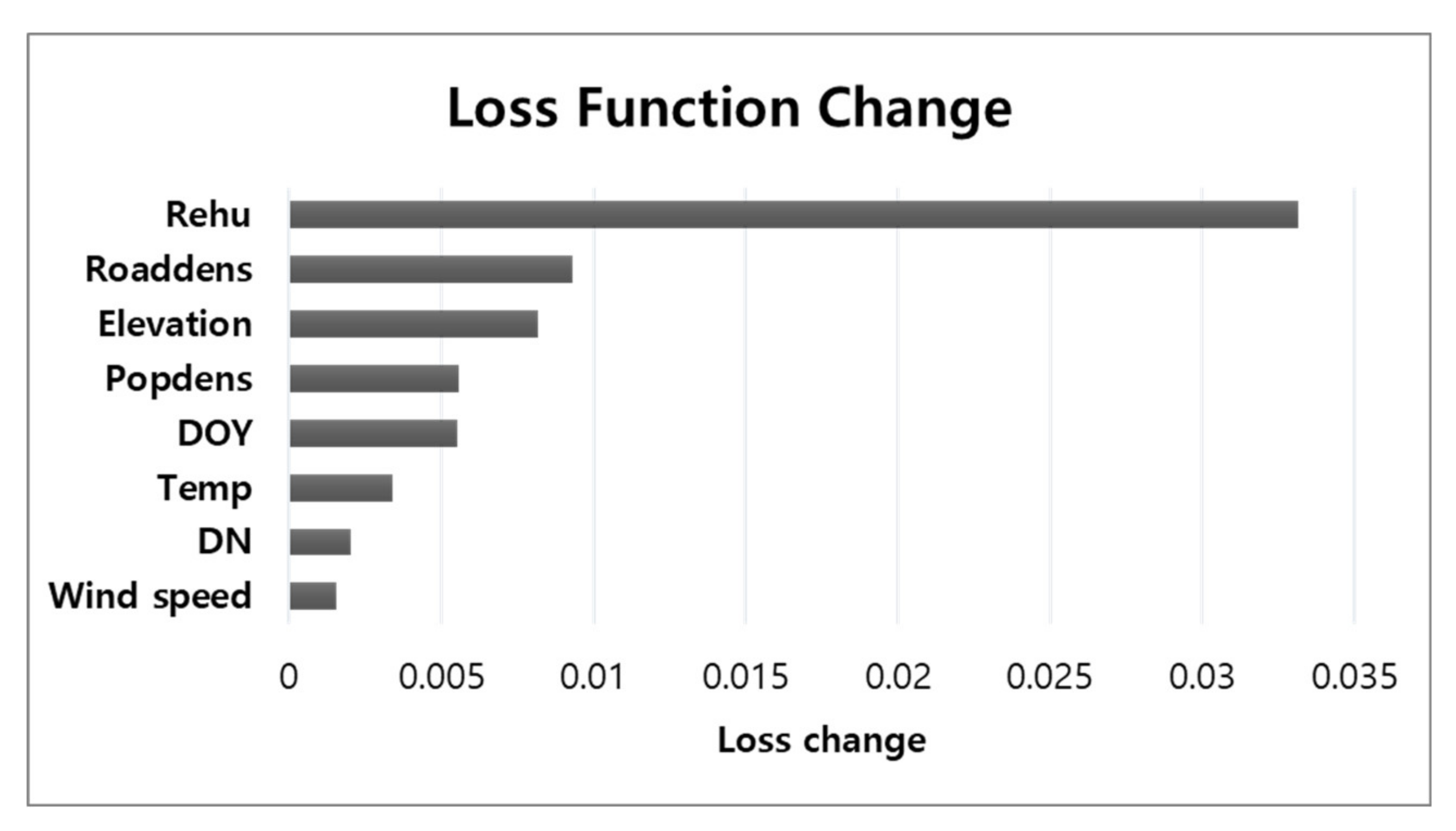
4.2. Feature Contribution Based on the Catboost Feature Importances

Figure 4 shows the feature importance identified by the integrated model based on the Loss function change. Rehu, Roaddens, Elevation, Popdens, and DOY in order were the top five contributing variables identified by Catboost. The most important variable was Rehu, which has been proved as a very useful and relevant variable representing dry weather conditions and dead fuel [20,60,61]. Rehu had a clearly opposite relationship with the number of forest fire cases considering their diurnal and seasonal patterns. Rehu has a peak in the dawn and decreases in the afternoon, and has a peak in summer and a decreasing pattern in winter and spring. The Pearson correlation coefficient of Rehu with HFRI was −0.8. Except for Rehu, contributing variables were closely related to accessibility, especially for the Roaddens, Elevation, and Popdens. The Pearson correlation coefficients of the three variables with HFRI were 0.4, −0.4, and 0.3, respectively. This agrees with the fact that most forest fire cases have occurred due to anthropogenic factors. The forest areas with high Roaddens, low Elevation, and high Podens have relatively high accessibility, which is vulnerable to forest fires [27]. DOY moderately contributed to the model. DOY is an effective factor for modeling the seasonality of forest fire risk: frequent forest fires in the dry season (spring and winter), while less in wet summer [62].
Figure 5a depicts the SHAP values of the variables calculated from the integrated model, which shows the degree of the positive or negative effect on the average of the predictions (i.e., the expected values) for all training data. Using the SHAP values, we investigated how each feature contributed to the prediction in the integrated model. This tendency is an overall summary of the SHAP values. It means each sample has a different contribution of each feature for the prediction. For example, when Rehu has a value close to the average rather than a particularly high or low value, the contribution of Roaddens or Elevation to the prediction is much greater. These interactions between features are analyzed with a dependence plot (Figure 5b).
SHAP values enable to identify how each feature affects the prediction when the feature has a certain value. In Figure 5a, the higher Rehu has negative contribution to the prediction up to −0.2. On the other hand, when the Rehu was low, it has positive contribution to the prediction up to 0.13. The high elevation decreased HFRI. While the low elevation increased the prediction, its effect was smaller than the decreasing effect. When the Roaddens was high, it increased the prediction. When Roaddens was lower, the prediction was lowered. Popdens was inversely related to elevation. It can be inferred that many of the samples predicted as low risk were determined mainly based on the influence of Rehu, elevation, and Roaddens. The weakness of the process of determining the forest fire risk through these three variables is that areas with low Roaddens and high elevation always result in low forest fire risk. It is because Rehu is a dynamic variable, so it reflects the situation at all times, but elevation and Roaddens are static variables. Therefore, it can be seen that the accessibility factors are very important in simulating forest fire risk. These results show the necessity of ensemble the meteorological model to complement the integrated model.
Figure 5b shows how Rehu works in the model depending on the Roaddens feature value. The SHAP value was close to 0 when the Rehu value was near 50. If the Rehu had a moderate value, a static forest fire risk map might be generated since the prediction was mostly determined by Elevation, Roaddens, and Popdens. The interaction between the Rehu and the Roaddens changed from the Rehu feature value of 50. When the Rehu was less than 50, it had a larger positive SHAP value with the low Roaddens. This is because if the Rehu was low and the road density was high, both features have the same direction to high forest fire risk, which leads to the relative reduction of the Rehu’s contribution. However, if the Roaddens was low despite the outbreak of a forest fire, the contribution of low Rehu would increase. This means that the contribution to the prediction varies depending on the feature value and the interaction between features.

4.3. Comparison of Percentile Rank between HFRI, Revised FFMC, and DWI

HFRI was compared to the revised FFMC and DWI using the percentile rank. To confirm the spatial accuracy, the percentile ranks of the forest fire pixels were calculated targeting all forest pixels every hour. Even if the indices (i.e., HFRI and DWI) have different ranges and distributions, since each index is spatially ordered for every pixel, it can be used to compare them which one is better at the discrimination between forest fire (representing high risk) and non-fire locations. For example, the percentile rank value of 95 means that the pixel is at the top 5% among all forest pixels at that time. Figure 6 shows the box plot of the percentile ranks of forest fire pixels.
The mean percentile ranks of all forest fire pixels were 68, 59, 61 for HFRI, revised FFMC, and DWI, respectively. Revised FFMC and DWI had the almost same mean values but that of DWI was slightly higher, while HFRI had a remarkably higher mean value than the other two indices. The most noticeable part here is that the percentage of forest fire pixels with a percentile rank of 90 or higher in HFRI is 30%, whereas the other two indices were only 20%. Moreover, the percentage of forest fires with a percentile rank of over 50 was 72%, whereas 65% for DWI and 61% for the revised FFMC. HFRI showed a higher mean percentile rank than DWI thanks to the integrated model. When comparing the percentile rank of HFRI-I and HFRI-M, the percentile rank of HFRI-I appears at the same level as that of HFRI, whereas the percentile rank of HFRI-M is similar to that of DWI developed based on weather factors. Since the integrated model is focused on extracting high-risk areas by sampling non-fire samples only at the time of forest fire and using accessibility factors together, it could have a higher percentile rank in forest fire areas. Therefore, it can be said that HFRI simulates the forest fire risk better in spatial detail and accuracy than the DWI. Since the DWI showed better results than the revised FFMC, the DWI was used in the subsequent analysis and comparison to HFRI.
Although HFRI had a high mean percentile rank, some forest fire pixels had values below 50. Such pixels were generally found in the spring (i.e., 74% in March and April) when forest fires were frequent. In the spring, the forest fire risk was high nationwide and many forest fire cases (e.g., 7) occurred at the same time. In that situation, the percentile rank of the forest fire pixels may be relatively lowered because the forest fire risk was nationwide high. However, it does not mean HFRI failed to simulate the forest fire risk because the actual forest fire risk index was high and only about 5–6% of the forest fire cases occurred in March and April fell into this category.

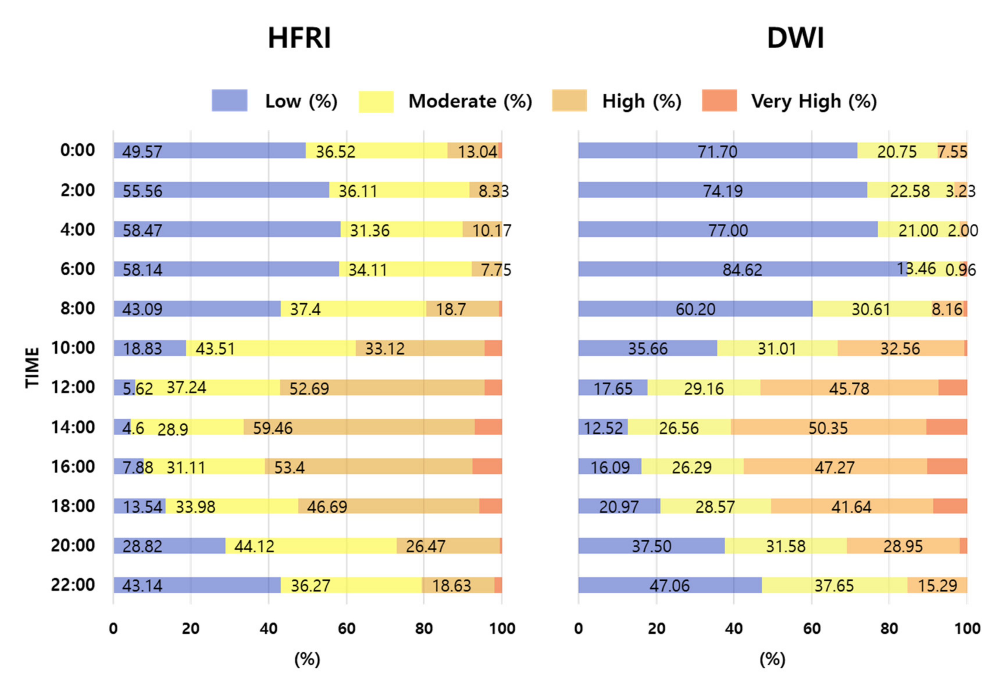
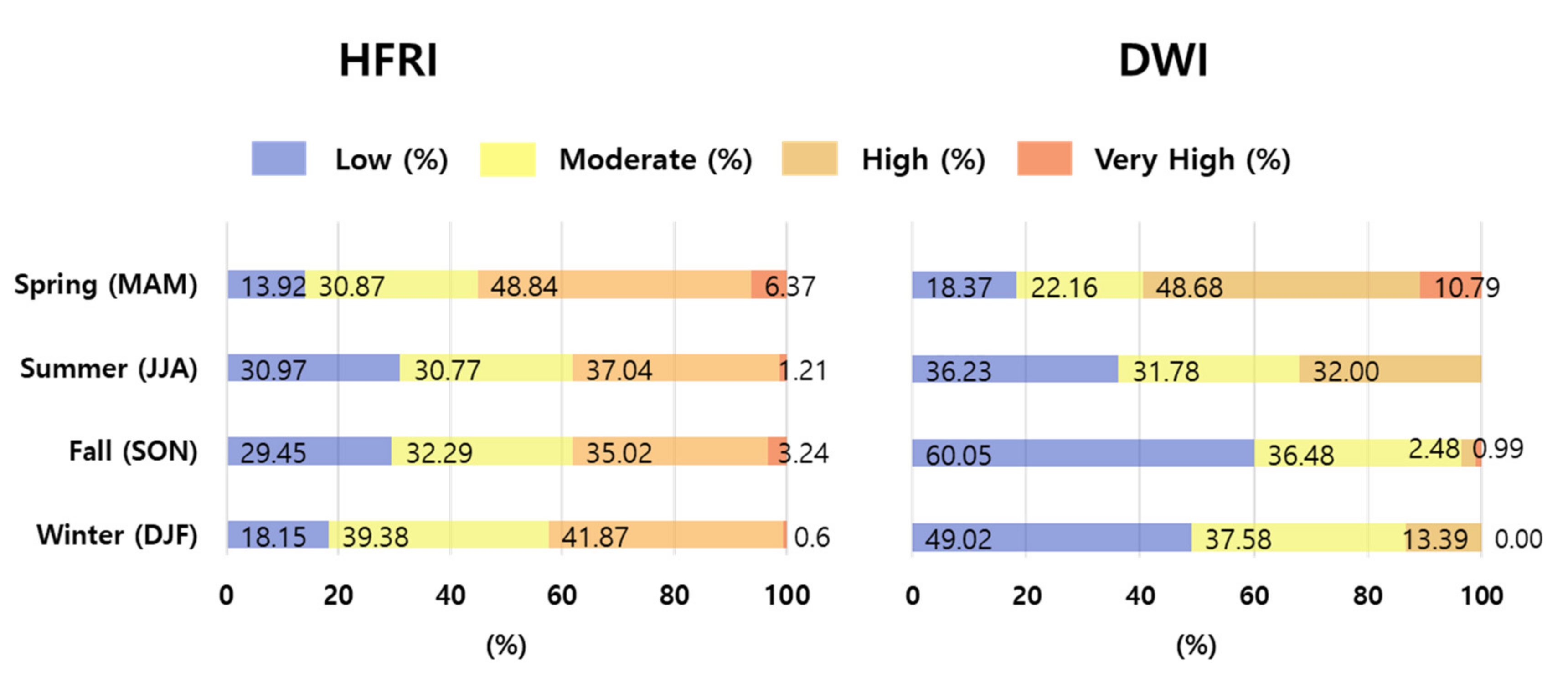
4.4. Comparison of Forest Fire Risk Classes between HFRI and DWI

In this section, HFRI and DWI distributions by risk class were examined using the results of one year out cross-validation by time and season. Figure 7 shows the classification result of HFRI and DWI for forest fires using machine learning validation data with a two-hour interval from 0:00 to 24:00 KST (local time). The sum of the values in each time zone is 100% and the value for each risk class is the proportion of the forest fire pixels for the corresponding time zone. Both HFRI and DWI produced good performances in the afternoon from 12:00 to 16:00 local time, showing many forest fires occurred in the high risk pixels. However, about 50% and 70% of the forest fires occurred in the early morning and at night (22:00–08:00) had low risk for HFRI and DWI, respectively. This is because both HFRI and DWI are affected by the temporal distribution of forest fires since they are empirical models: samples were not evenly distributed on the temporal domain. Forest fires tend to occur intensively in the afternoon (Supplementary Figure S3), increasing the forest fire risk index. Oppositely, the forest fire risk was low in the early morning and night when there were fewer forest fires. Although a majority of forest fires in the early morning and at night were classified as low class, the actual average number of forest fires classified as low class in the early morning and at night was only up to 58 because the absolute number of forest fires was very small when compared to the afternoon.
The largest difference in the proportion between the two indices was observed in low class. For HFRI, the proportion of low class for all times decreased by at least 3.9% up to 26.5% when compared to the DWI. Although both indices rapidly dropped in the morning (6:00–12:00), the rate of Low class was much lower for HFRI than the DWI. While the rate of Moderate and High classes was much larger for HFRI than the DWI at dawn and early morning. It is due to the high relative humidity and very low temperature in the early morning, which play an important role in calculating DWI. The average Rehu of forest fire pixels occurring in the dawn and morning (from 00:00 to 10:00) was 62.4%, which was higher than the average Rehu of 43.4% at the other times (from 11:00 to 23:00). Interestingly, the average values of the Popdens and Roaddens of forest fire pixels at dawn and early morning were 1683 and 179, respectively, higher than the other times (1295 and 150, respectively), which implies that accessibility increased the risk even at that time. In other words, DWI, simply based on the meteorological conditions, has limitations in simulating the forest fire risk at dawn and early morning, while HFRI improved them by incorporating anthropogenic features in addition to weather conditions.
Figure 8 shows the classification results of HFRI and DWI by season. Both HFRI and DWI well simulated the forest fire risk in spring. However, they showed limited performance in summer and fall. DWI did not work well for winter, either. This might be because empirical modeling approaches were used for both indices with the use of much larger sample size in spring than other seasons. The results of the two indices in spring and summer showed almost similar patterns, but very different in fall and winter. In the DWI, the rate of forest fire occurrences in high class in fall and winter rapidly decreased, and most of the forest fires occurred in low class. On the other hand, in HFRI, the proportion of high class was high in fall and winter resulting in a decrease of 30.6 and 30.87% in low class when compared to the DWI. The mean Rehu of forest fire pixels in fall (52%) had the higher value than in spring and winter (40% and 45%), resulting in less prone to forest fires. For these reasons, the percentage of the high class both HFRI and DWI declined in fall. Nevertheless, HFRI was more likely to be classified as high risk compared to DWI because the relative influence of the Rehu was offset by other factors in HFRI. Overall, the low class rate for HFRI was lower than for DWI for all seasons. In addition, the class rates of HFRI did not change much by season, while those of DWI dramatically changed, which implies the temporal robustness of HFRI over DWI.

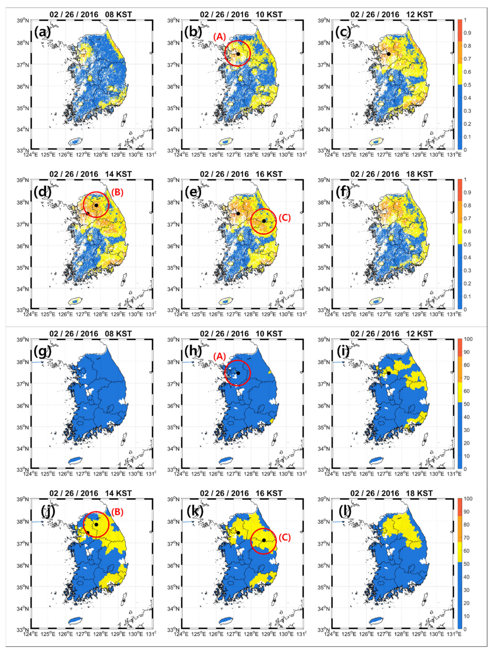
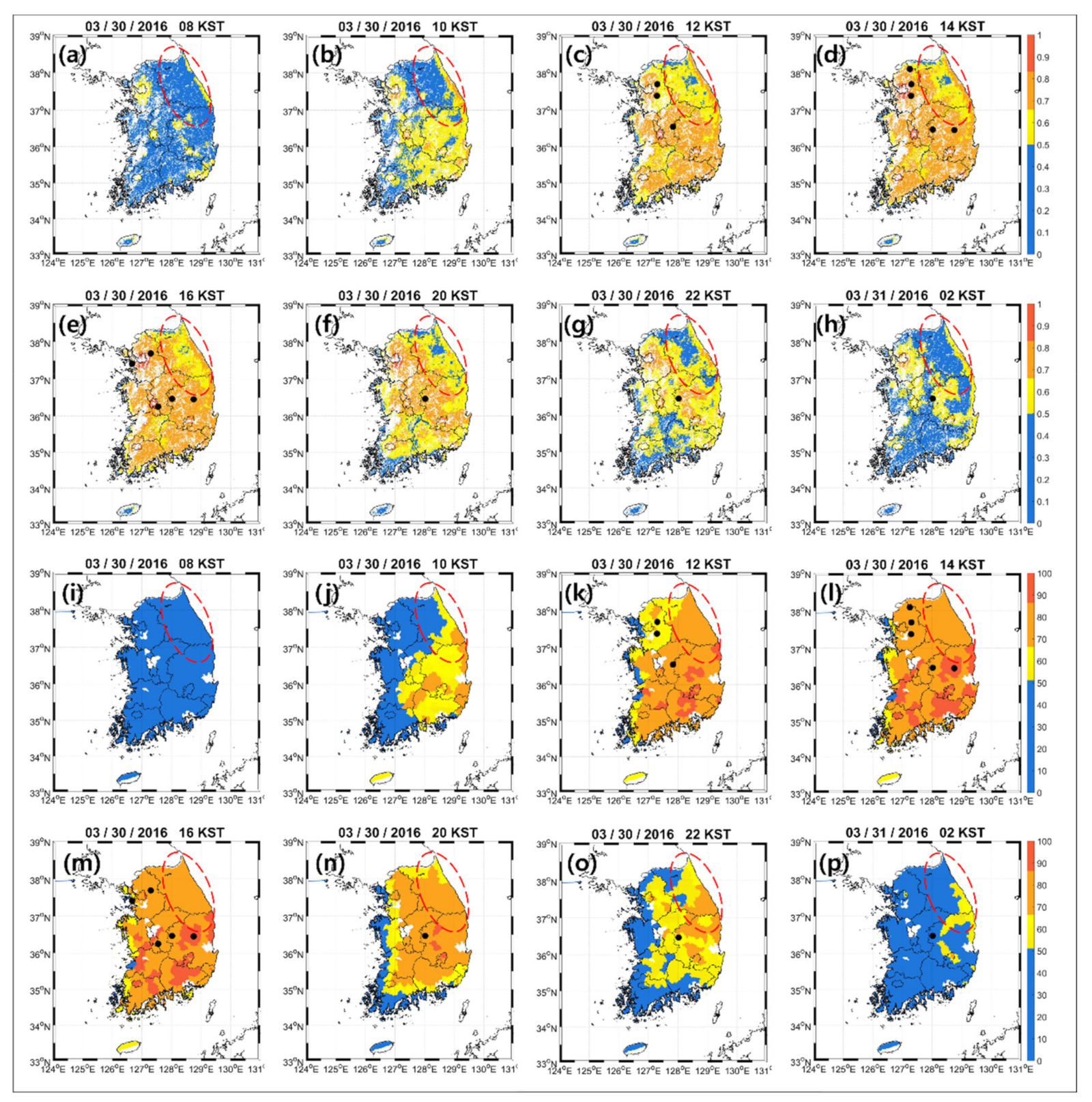
4.5. Mapping Results of HFRI and DWI

Figure 9 shows the spatial distribution of two indices (i.e., HFRI and DWI) with a two-hour interval on 25 February 2016 with three forest fire cases. The difference in spatial distribution of two indices over time and the advantages of the fine spatial resolution of HFRI are described in Figure 7. Both HFRI and DWI had similar spatial distributions overall, and the high forest fire risk areas were well-matched with actual fire locations. This is because both HFRI and DWI are largely influenced by Rehu, which is a common factor.
However, as mentioned in Figure 7, DWI was not able to detect the forest fire risk in the morning compared to HFRI. This is well illustrated on the map at 10:00 KST (Figure 9b,h). Despite the forest fire occurred in Gwangju at 9:55, that area was classified as Low class of DWI (Figure 9h), but the high class of HFRI (Figure 9b). Moreover, as mentioned in Figure 8, DWI was not able to detect the forest fires well in winter when compared to HFRI. Forest fires usually occurred in low class of DWI in winter, while HFRI well detected them in high class. This supports that HFRI is stable regardless of season, showing the advantages of more detailed spatial variations within administrative districts.
Figure 10 shows the spatial distribution of HFRI and DWI from 30 to 31 March 2016 with a total of 7 forest fires. According to Figure 7 and Figure 8, DWI has almost the same rate as the High class with HFRI from 10:00 to 20:00 in spring. Therefore, the spatiotemporal patterns between the two indices in spring are examined in Figure 10.
On the map from 12:00 on March 30 to 2:00 on 31 March, the forest fire risk at the fire location matched a relatively high risk zone in both HFRI and DWI. On the other hand, paying attention to the circle with a dashed red line where the forest fire did not occur, HFRI showed a relatively lower risk distribution (low or moderate) on the red circle region than the location of the fires. However, the DWI has a nationally high class (high and very high) in the afternoon and early evening in the region with the red circle. In particular, the 20:00 maps (Figure 10f,n) show that the DWI still showed a high-risk across the country (Figure 10n), compared to HFRI that has a high risk mainly around the forest fire location and lower risk in other areas (Figure 10f). In spring, the forest fire risk naturally rises due to dry and warm weather so the DWI tended to overestimate the fire risk. Thus, the proportion of forest fires that occurred in high class rapidly increased in the afternoon in spring. On the other hand, HFRI can simulate the detailed forest fire risk in a single administrative district with fine resolutions so it did not show excessively high risk spatial distribution over a large area. Furthermore, the maps from 22:00 on 30 March and 2:00 on 31 March (Figure 10g,h,o,p) showed that HFRI had a relatively high risk at the forest fire location while the DWI had a low risk. This confirms that DWI did not work well at night, resulting in a low risk even in spring, as shown in Figure 7.

5. Conclusions

Existing forest fire risk indices as an operational use are mostly based on weather and fuel data, and often require complex processes through various conditions based on statistics. In this study, a new hourly forest fire risk index (HFRI) based on the Catboost machine learning using various factors including weather, accessibility, and fuel data was proposed over South Korea. HFRI is provided by the ensemble model that linearly combined the integrated and meteorological models with different input variables. HFRI was validated through the ROC curves and AUC values, and compared to the revised FFMC and DWI through the percentile rank. The AUC of HFRI was 0.8434, much higher than the meteorological model (i.e., typical fire risk model). Moreover, HFRI has shown stable performance in identifying forest fire risk areas dynamically with diurnal and seasonal change. In addition, spatial variations exist within administrative districts because of their fine resolution (1km), which can also help deploy forest fire fighting resources at the district level. However, since HFRI uses local forest density data and the numerical model (i.e., digital forecast model) available in the study area, it is necessary to replace them with globally available data (e.g., Global Data Assimilation and Prediction System) to improve the transferability of the index. In addition, the causes of forest fires may vary by region, it is crucial to extensively train and evaluate the index over multiple areas with different characteristics of forest fires.
Feature contribution analysis through SHAP values showed that Rehu had the greatest contribution, followed by elevation, Roaddens, and Popdens, in order. Most of the contributing features were related to the accessibility, implying that such features were critical especially for areas with frequent forest fires caused by anthropogenic reasons. Due to these static accessibility variables, the high forest fire risk was generally concentrated around urban areas even though HFRI was complemented through the ensemble model structure with the meteorological model. In the future, improved performance is expected if additional spatiotemporally dynamic accessibility variables, such as the number of floating population and the number of hikers by date, are incorporated in the ensemble model.

Supplementary Materials

The following are available online at https://www.mdpi.com/2076-3417/10/22/8213/s1, Figure S1: SHAP value for elevation data, Figure S2: HFRI (ensemble model) (a–d) and the integrated model(e–h) maps with the four-hour interval, and Figure S3: The forest fire sample distribution by time.

Author Contributions

Conceptualization, Y.K. and J.I.; methodology, Y.K., E.J., and J.I.; validation, Y.K. and E.J.; formal analysis, Y.K. and E.J.; investigation, Y.K. and E.J.; data curation, C.K., and S.K.; writing—original draft preparation, Y.K.; writing—review and editing, E.J., J.I, C.K., and S.K.; visualization, Y.K.; supervision, J.I. All authors have read and agreed to the published version of the manuscript.

Funding

This research was supported by a grant (no.20009742) of Disaster-Safety Industry Promotion Program funded by Ministry of Interior and Safety (MOIS, Korea) and by a grant from the National Institute of Forest Science, Korea, grant number F0500-2018-01. Y.K. was supported by Basic Science Research Program through the National Research Foundation of Korea (NRF) funded by the Ministry of Education (NRF-2020R1A6A3A13075983).

Conflicts of Interest

The authors declare no conflict of interest.

References

  1. Van Hoang, T.; Chou, T.Y.; Fang, Y.M.; Nguyen, N.T.; Nguyen, Q.H.; Xuan Canh, P.; Ngo Bao Toan, D.; Nguyen, X.L.; Meadows, M.E. Mapping Forest Fire Risk and Development of Early Warning System for NW Vietnam Using AHP and MCA/GIS Methods. Appl. Sci. 2020, 10, 4348. [Google Scholar] [CrossRef]
  2. Mallinis, G.; Mitsopoulos, I.; Chrysafi, I.J.G.; Sensing, R. Evaluating and comparing Sentinel 2A and Landsat-8 Operational Land Imager (OLI) spectral indices for estimating fire severity in a Mediterranean pine ecosystem of Greece. GISci. Remote Sens. 2018, 55, 1–18. [Google Scholar] [CrossRef]
  3. Gelabert, P.; Montealegre, A.; Lamelas, M.; Domingo, D.J.G.; Sensing, R. Forest structural diversity characterization in Mediterranean landscapes affected by fires using Airborne Laser Scanning data. GISci. Remote Sens. 2020, 57, 497–509. [Google Scholar] [CrossRef]
  4. Abdollahi, M.; Islam, T.; Gupta, A.; Hassan, Q.K. An advanced forest fire danger forecasting system: Integration of remote sensing and historical sources of ignition data. Remote Sens. 2018, 10, 923. [Google Scholar] [CrossRef] [Green Version]
  5. Laneve, G.; Pampanoni, V.; Shaik, R.U. The Daily Fire Hazard Index: A Fire Danger Rating Method for Mediterranean Areas. Remote Sens. 2020, 12, 2356. [Google Scholar] [CrossRef]
  6. Cheret, V.; Denux, J.-P.J.G.; Sensing, R. Analysis of MODIS NDVI time series to calculate indicators of Mediterranean forest fire susceptibility. GISci. Remote Sens. 2011, 48, 171–194. [Google Scholar] [CrossRef]
  7. Gigović, L.; Pourghasemi, H.R.; Drobnjak, S.; Bai, S. Testing a new ensemble model based on SVM and random forest in forest fire susceptibility assessment and its mapping in Serbia’s Tara National Park. Forests 2019, 10, 408. [Google Scholar] [CrossRef] [Green Version]
  8. Zhang, G.; Wang, M.; Liu, K. Forest fire susceptibility modeling using a convolutional neural network for Yunnan province of China. Int. J. Disaster Risk Sci. 2019, 10, 386–403. [Google Scholar] [CrossRef] [Green Version]
  9. Pham, B.T.; Jaafari, A.; Avand, M.; Al-Ansari, N.; Dinh Du, T.; Yen, H.P.H.; Phong, T.V.; Nguyen, D.H.; Le, H.V.; Mafi-Gholami, D. Performance evaluation of machine learning methods for forest fire modeling and prediction. Symmetry 2020, 12, 1022. [Google Scholar] [CrossRef]
  10. Hong, H.; Tsangaratos, P.; Ilia, I.; Liu, J.; Zhu, A.-X.; Xu, C. Applying genetic algorithms to set the optimal combination of forest fire related variables and model forest fire susceptibility based on data mining models. The case of Dayu County, China. Sci. Total Environ. 2018, 630, 1044–1056. [Google Scholar] [CrossRef]
  11. Bui, D.T.; Bui, Q.-T.; Nguyen, Q.-P.; Pradhan, B.; Nampak, H.; Trinh, P.T. A hybrid artificial intelligence approach using GIS-based neural-fuzzy inference system and particle swarm optimization for forest fire susceptibility modeling at a tropical area. Agric. For. Meteorol. 2017, 233, 32–44. [Google Scholar]
  12. Sachdeva, S.; Bhatia, T.; Verma, A. GIS-based evolutionary optimized Gradient Boosted Decision Trees for forest fire susceptibility mapping. Nat. Hazards 2018, 92, 1399–1418. [Google Scholar] [CrossRef]
  13. Karali, A.; Roussos, A.; Giannakopoulos, C.; Hatzaki, M.; Xanthopoulos, G.; Kaoukis, K. Evaluation of the Canadian Fire Weather Index in Greece and future climate projections. In Advances in Meteorology, Climatology and Atmospheric Physics; Springer: Berlin/Heidelberg, Germany, 2013; pp. 501–508. [Google Scholar]
  14. Tian, X.; McRae, D.J.; Jin, J.; Shu, L.; Zhao, F.; Wang, M. Wildfires and the Canadian Forest Fire Weather Index system for the Daxing’anling region of China. Int. J. Wildland Fire 2012, 20, 963–973. [Google Scholar] [CrossRef]
  15. Ziel, R.H.; Bieniek, P.A.; Bhatt, U.S.; Strader, H.; Rupp, T.S.; York, A. A Comparison of Fire Weather Indices with MODIS Fire Days for the Natural Regions of Alaska. Forests 2020, 11, 516. [Google Scholar] [CrossRef]
  16. Dimitrakopoulos, A.; Bemmerzouk, A.; Mitsopoulos, I. Evaluation of the Canadian fire weather index system in an eastern Mediterranean environment. Meteorol. Appl. 2011, 18, 83–93. [Google Scholar] [CrossRef]
  17. Jeong, J.-Y.; Woo, S.-H.; Son, R.-H.; Yoon, J.-H.; Jeong, J.-H.; Lee, S.-J.; Lee, B.-D. Spring Forest-Fire Variability over Korea Associated with Large-Scale Climate Factors. Atmosphere 2018, 28, 457–467. [Google Scholar]
  18. De Jong, M.C.; Wooster, M.J.; McCall, F.F. Calibration and evaluation of the Canadian Forest Fire Weather Index (FWI) System for improved wildland fire danger rating in the United Kingdom. Nat. Hazards Earth Syst. Sci. 2016, 16, 1217. [Google Scholar] [CrossRef] [Green Version]
  19. Van Wagner, C.; Forest, P. Development and Structure of the Canadian Forest Fire Weather Index System; Canadian Forestry Service Headquarters: Ottawa, ON, Canada, 1987. [Google Scholar]
  20. Satir, O.; Berberoglu, S.; Donmez, C. Mapping regional forest fire probability using artificial neural network model in a Mediterranean forest ecosystem. Geomat. Nat. Hazards Risk 2016, 7, 1645–1658. [Google Scholar] [CrossRef] [Green Version]
  21. Adab, H.; Atabati, A.; Oliveira, S.; Gheshlagh, A.M. Assessing fire hazard potential and its main drivers in Mazandaran province, Iran: A data-driven approach. Environ. Monit. Assess. 2018, 190, 670. [Google Scholar] [CrossRef]
  22. Viedma, O.; Urbieta, I.; Moreno, J. Wildfires and the role of their drivers are changing over time in a large rural area of west-central Spain. Sci. Rep. 2018, 8, 17797. [Google Scholar] [CrossRef] [Green Version]
  23. Won, M.; Jang, K.; Yoon, S. Development of the National Integrated Daily Weather Index (DWI) Model to Calculate Forest Fire Danger Rating in the Spring and Fall. Korean Soc. Agric. Meteorol. 2018, 20, 348–356. [Google Scholar]
  24. Won, M.; Yoon, S.; Jang, K. Developing Korean forest fire occurrence probability model reflecting climate change in the spring of 2000s. Korean J. Agric. For. Meteorol. 2016, 18, 199–207. [Google Scholar] [CrossRef] [Green Version]
  25. Kim, S.J.; Lim, C.-H.; Kim, G.S.; Lee, J.; Geiger, T.; Rahmati, O.; Son, Y.; Lee, W.-K.J.R.S. Multi-temporal analysis of forest fire probability using socio-economic and environmental variables. Remote Sens. 2019, 11, 86. [Google Scholar] [CrossRef] [Green Version]
  26. Ghorbanzadeh, O.; Blaschke, T.; Gholamnia, K.; Aryal, J. Forest fire susceptibility and risk mapping using social/infrastructural vulnerability and environmental variables. Fire 2019, 2, 50. [Google Scholar] [CrossRef] [Green Version]
  27. Pourtaghi, Z.S.; Pourghasemi, H.R.; Aretano, R.; Semeraro, T.J.E.i. Investigation of general indicators influencing on forest fire and its susceptibility modeling using different data mining techniques. Ecol. Indic. 2016, 64, 72–84. [Google Scholar] [CrossRef]
  28. Ricotta, C.; Bajocco, S.; Guglietta, D.; Conedera, M. Assessing the influence of roads on fire ignition: Does land cover matter? Fire 2018, 1, 24. [Google Scholar] [CrossRef] [Green Version]
  29. Korea Forest Service. Available online: http://www.forest.go.kr/newkfsweb/kfi/kfs/frfr/selectFrfrStats.do?searchCnd=2010&mn=KFS_02_02_01_05_01 (accessed on 19 August 2020).
  30. Ministry of Land, Infrastructure, and Transport, National Geographic Information Institute. Available online: http://map.ngii.go.kr/ms/pblictn/nationMapBook.do (accessed on 19 August 2020).
  31. Advanced Land Observing Satellite. Available online: https://www.eorc.jaxa.jp/ALOS/en/aw3d30/index.htm (accessed on 19 August 2020).
  32. Environmental Geographic Information. Available online: https://egis.me.go.kr/main.do (accessed on 19 August 2020).
  33. Won, M.; Lee, M.; Lee, W.; Yoon, S. Prediction of Forest Fire Danger Rating over the Korean Peninsula with the Digital Forecast Data and Daily Weather Index (DWI) Model. Korean Soc. Agric. Meteorol. 2012, 14, 1–10. [Google Scholar] [CrossRef]
  34. Srock, A.F.; Charney, J.J.; Potter, B.E.; Goodrick, S.L. The hot-dry-windy index: A new fire weather index. Atmosphere 2018, 9, 279. [Google Scholar] [CrossRef] [Green Version]
  35. Tadono, T.; Nagai, H.; Ishida, H.; Oda, F.; Naito, S.; Minakawa, K.; Iwamoto, H. Generation of the 30 M-mesh global digital surface model by ALOS PRISM. Int. Arch. Photogramm. Remote Sens. Spat. Inf. Sci. 2016, 41. [Google Scholar]
  36. Santillan, J.; Makinano-Santillan, M. Vertical accuracy assessment of 30-m resolution Alos, Aster, and SRTM global dems over northeastern Mindanao, Philippines. Int. Arch. Photogramm. Remote Sens. Spat. Inf. Sci. 2016, 41. [Google Scholar]
  37. Courty, L.G.; Soriano-Monzalvo, J.C.; Pedrozo-Acuña, A. Evaluation of open-access global digital elevation models (AW3D30, SRTM, and ASTER) for flood modelling purposes. J. Flood Risk Manag. 2019, 12, e12550. [Google Scholar] [CrossRef] [Green Version]
  38. Socioeconomic Data and Applications Center. Available online: https://sedac.ciesin.columbia.edu/data/set/gpw-v4-population-density-rev11/data-download (accessed on 19 August 2020).
  39. Global Roads Inventory Project. Available online: https://www.globio.info/download-grip-dataset (accessed on 19 August 2020).
  40. Meijer, J.R.; Huijbregts, M.A.; Schotten, K.C.; Schipper, A.M. Global patterns of current and future road infrastructure. Environ. Res. Lett. 2018, 13, 064006. [Google Scholar] [CrossRef] [Green Version]
  41. Forest Geospatial Information System. Available online: http://www.forest.go.kr/newkfsweb/kfs/idx/SubIndex.do?orgId=fgis&mn=KFS_03_08_01 (accessed on 19 August 2020).
  42. Zhan, Y.; Luo, Y.; Deng, X.; Chen, H.; Grieneisen, M.L.; Shen, X.; Zhu, L.; Zhang, M.J.A.e. Spatiotemporal prediction of continuous daily PM2. 5 concentrations across China using a spatially explicit machine learning algorithm. Atmos. Environ. 2017, 155, 129–139. [Google Scholar] [CrossRef]
  43. Park, S.; Shin, M.; Im, J.; Song, C.-K.; Choi, M.; Kim, J.; Lee, S.; Park, R.; Kim, J.; Lee, D.-W. Estimation of ground-level particulate matter concentrations through the synergistic use of satellite observations and process-based models over South Korea. Atmos. Chem. Phys. 2019, 19, 1097–1113. [Google Scholar] [CrossRef] [Green Version]
  44. Franke, G.R. Multicollinearity. In Wiley International Encyclopedia of Marketing; Wiley: Hoboken, NJ, USA, 2010. [Google Scholar]
  45. Tien Bui, D.; Hoang, N.-D.; Samui, P. Spatial pattern analysis and prediction of forest fire using new machine learning approach of Multivariate Adaptive Regression Splines and Differential Flower Pollination optimization: A case study at Lao Cai province (Viet Nam). J. Environ. Manag. 2019, 237, 476–487. [Google Scholar] [CrossRef] [PubMed]
  46. Bentéjac, C.; Csörgő, A.; Martínez-Muñoz, G. A comparative analysis of gradient boosting algorithms. Artif. Intell. Rev. 2020, 1–31. [Google Scholar] [CrossRef]
  47. Huang, G.; Wu, L.; Ma, X.; Zhang, W.; Fan, J.; Yu, X.; Zeng, W.; Zhou, H. Evaluation of CatBoost method for prediction of reference evapotranspiration in humid regions. J. Hydrol. 2019, 574, 1029–1041. [Google Scholar] [CrossRef]
  48. Prokhorenkova, L.; Gusev, G.; Vorobev, A.; Dorogush, A.V.; Gulin, A. CatBoost: Unbiased boosting with categorical features. In Proceedings of the 32nd International Conference on Neural Information Processing Systems, Canada, December 2018; Bengio, S., Wallach, H.M., Larochelle, H., Grauman, K., Cesa-Bianchi, N., Eds.; Curran Associates Inc.: Red Hook, NY, USA, 2018. [Google Scholar]
  49. Lundberg, S.M.; Lee, S.-I. A unified approach to interpreting model predictions. In Proceedings of the Advances in Neural Information Processing Systems; MIT Press: Cambridge, MA, USA, 1999; pp. 4765–4774. [Google Scholar]
  50. Zhang, Y.; Zhao, Z.; Zheng, J. CatBoost: A new approach for estimating daily reference crop evapotranspiration in arid and semi-arid regions of Northern China. J. Hydrol. 2020, 588, 125087. [Google Scholar] [CrossRef]
  51. Catboost. Available online: https://catboost.ai/ (accessed on 21 October 2020).
  52. Pan, J.; Wang, W.; Li, J. Building probabilistic models of fire occurrence and fire risk zoning using logistic regression in Shanxi Province, China. Nat. Hazards 2016, 81, 1879–1899. [Google Scholar] [CrossRef]
  53. Regmi, N.R.; Giardino, J.R.; Vitek, J.D. Modeling susceptibility to landslides using the weight of evidence approach: Western Colorado, USA. Geomorphology 2010, 115, 172–187. [Google Scholar] [CrossRef]
  54. Pourghasemi, H.R.; Mohammady, M.; Pradhan, B. Landslide susceptibility mapping using index of entropy and conditional probability models in GIS: Safarood Basin, Iran. CATENA 2012, 97, 71–84. [Google Scholar] [CrossRef]
  55. Abedi Gheshlaghi, H.; Feizizadeh, B.; Blaschke, T. GIS-based forest fire risk mapping using the analytical network process and fuzzy logic. J. Environ. Plan. Manag. 2020, 63, 481–499. [Google Scholar] [CrossRef]
  56. Adab, H.; Kanniah, K.D.; Solaimani, K. Modeling forest fire risk in the northeast of Iran using remote sensing and GIS techniques. Nat. Hazards 2013, 65, 1723–1743. [Google Scholar] [CrossRef]
  57. Tehrany, M.S.; Jones, S.; Shabani, F.; Martínez-Álvarez, F.; Bui, D.T. A novel ensemble modeling approach for the spatial prediction of tropical forest fire susceptibility using logitboost machine learning classifier and multi-source geospatial data. Theor. Appl Climatol. 2019, 137, 637–653. [Google Scholar] [CrossRef]
  58. Kang, Y.; Park, S.; Jang, E.; Im, J.; Kwon, C.; Lee, S. Spatio-temporal enhancement of forest fire risk index using weather forecast and satellite data in South Korea. J. Korean Assoc. Geogr. Inf. Stud. 2019, 22, 116–130. [Google Scholar]
  59. Park, H.; Lee, S.; Chae, H.; Lee, W. A Study on the Development of Forest Fire Occurrence Probability Model using Canadian Forest Fire Weather Index -Occurrence of Forest Fire in Kangwon Province. J. Korean Soc. Hazard Mitig. 2009, 9, 95–100. [Google Scholar]
  60. Chowdhury, E.H.; Hassan, Q.K. Development of a new daily-scale forest fire danger forecasting system using remote sensing data. Remote Sens. 2015, 7, 2431–2448. [Google Scholar] [CrossRef] [Green Version]
  61. Bedia, J.; Golding, N.; Casanueva, A.; Iturbide, M.; Buontempo, C.; Gutiérrez, J.M. Seasonal predictions of Fire Weather Index: Paving the way for their operational applicability in Mediterranean Europe. Clim. Serv. 2018, 9, 101–110. [Google Scholar] [CrossRef]
  62. Acosta, M.; Darenova, E.; Krupková, L.; Pavelka, M. Seasonal and inter-annual variability of soil CO2 efflux in a Norway spruce forest over an eight-year study. Agric. For. Meteorol. 2018, 256–257, 93–103. [Google Scholar] [CrossRef]
Figure 1. The study area of South Korea with (a) elevation and (b) land cover data. The elevation data come from ALOS World 3D 30m v3.1 [31]. The land cover data were provided by the Ministry of Environment [32].
Applsci 10 08213 g001
Figure 2. Process flow diagram of the proposed approach in this study.
Applsci 10 08213 g002
Figure 3. The one-year-out cross-validation ROC curves. (af) are the one-year-out cross-validation ROC curves for individual years, and (g) is the ROC curve for the entire study period.
Applsci 10 08213 g003
Figure 4. The Loss function change feature importance of Catboost machine learning from the integrated model.
Applsci 10 08213 g004
Figure 5. (a) is the summary plot of SHAP values in Catboost machine learning from the integrated model. The horizontal position means the impact of a feature value for prediction. The thickness and color indicate the sample size and original value for each feature, respectively. The feature with a large impact on prediction is located at the top. (b) is the SHAP value dependence plot between Rehu and Roaddens. The X-axis is the feature value of Rehu. The Y-axis is the SHAP value for Rehu. The color means the feature value of Roaddens.
Applsci 10 08213 g005
Figure 6. The comparison of five models with percentile rank every hour. HFRI- I, M are the integrated model and the meteorological model, respectively. The left side is the box plot of each model percentile rank for forest fires. In the box plot, cases between 25 and 75% are displayed as boxes, and the red line means the average value. On the right side of the box plot, the percentage of the total forest fires in each section is additionally displayed.
Applsci 10 08213 g006
Figure 7. HFRI and DWI classes by the time with two hours interval. The total sum of each time for each index is 100%, indicating how many forest fires fall into this class as a percentage form.
Applsci 10 08213 g007
Figure 8. HFRI and DWI classes by season. The total sum of each time for each index is 100%, indicating how many forest fires fall into this class as a percentage form.
Applsci 10 08213 g008
Figure 9. HFRI (af) and DWI (gl) maps with the two-hour interval in winter. The black dots are forest fire locations. There were three forest fires in February 26, 2016: (A) Gwangju during the 9:55–18:00 KST, (B) Chuncheon during the 14:43–15:35 KST, and (C) Yeongwol during the 15:40–16:15 KST. HFRI was masked using a forest land cover type to produce results only in forest regions in (af). If there are missing values in DWI, they are displayed as No data (white color).
Applsci 10 08213 g009
Figure 10. HFRI (ah) and DWI (ip) maps in spring. The black dots are forest fires. There are seven forest fires. If there is no data due to the missing data from DWI, the next time data was used. Thus, the map was displayed as a time series at intervals of 2 or 4 h.
Applsci 10 08213 g010
Table 1. Data description used for machine learning model building.
DataSourceVariablesAbbreviation
Weather dataKorea Meteorological AdministrationRelative humidityRehu
TemperatureTemp
Wind speedWind speed
Geographical dataJAXA ALOSAW3D30 v3.1Elevation
NASA Gridded Population of the World (GPW), v4Populated area rasterPopdens
GRIP global roads datasetRoad vectorRoaddens
Fuel dataForest Geospatial Information SystemForest densityDN
Time-related data Day of the YearDOY
Table 2. Assigned values for fire and non-fire samples, representing very high and low fire risk respectively, based on the monthly forest fire density. X denotes the monthly forest fire density percentile value for each pixel.
Monthly Forest Fire Density Percentile0 ≤ X < 2525 ≤ X < 5050 ≤ X < 7575 ≤ X
Assigned valuesFire1
Non-fire00.10.2-
Table 3. The number of fire and non-fire samples for the integrated model and the meteorological model. For simple representation, the time scale of the hour is displayed at two-time interval. The fire and non-fire samples were classified according to the time of occurrence (i.e., hour, season, and year), and then the total number of samples is shown in the table.
Time ScaleFireNon-Fire for the Integrated ModelNon-Fire for the Meteorological Model
Hour
0:00180140771
2:00168129787
4:00182129783
6:00196154782
8:00183154787
10:00236190805
12:00664502948
14:0011769061202
16:0010859341123
18:00531402866
20:00263197829
22:00165131771
Season
Spring577543026448
Summer150311975032
Fall7176025002
Winter200115424419
Year
2014130113283396
2015201812883641
2016117612923549
2017218412043394
2018156212753417
2019175512563504
Table 4. Forest fire risk classes and their intervals for Hourly Forest fire Risk Index (HFRI) and Daily Weather Index (DWI).
IndexClass
LowModerateHighVery High
HFRI0–0.490.5–0.660.67–0.830.84–1
DWI0–5051–6566–8586–100
Publisher’s Note: MDPI stays neutral with regard to jurisdictional claims in published maps and institutional affiliations.

