SAR and LIDAR Datasets for Building Damage Evaluation Based on Support Vector Machine and Random Forest Algorithms—A Case Study of Kumamoto Earthquake, Japan

Abstract

The evaluation of buildings damage following disasters from natural hazards is a crucial step in determining the extent of the damage and measuring renovation needs. In this study, a combination of the synthetic aperture radar (SAR) and light detection and ranging (LIDAR) data before and after the earthquake were used to assess the damage to buildings caused by the Kumamoto earthquake. For damage assessment, three variables including elevation difference (ELD) and texture difference (TD) in pre- and post-event LIDAR images and coherence difference (CD) in SAR images before and after the event were considered and their results were extracted. Machine learning algorithms including random forest (RDF) and the support vector machine (SVM) were used to classify and predict the rate of damage. The results showed that ELD parameter played a key role in identifying the damaged buildings. The SVM algorithm using the ELD parameter and considering three damage rates, including D0 and D1 (Negligible to slight damages), D2, D3 and D4 (Moderate to Heavy damages) and D5 and D6 (Collapsed buildings) provided an overall accuracy of about 87.1%. In addition, for four damage rates, the overall accuracy was about 78.1%.

1. Introduction

Immediate response and planning for rescue and reconstruction operations are essential after an earthquake. Field survey is time-consuming and costly and, in some cases, this is impossible due to road closures [1,2,3,4]. Hence, several remote sensing datasets and methods have been proposed to accelerate this work. One of the best ways to assess earthquake damage is to use space borne and airborne information before and after the event [5]. Synthetic aperture radar (SAR) is one of the most powerful tools for monitoring natural and unnatural events on Earth that can collect information during the day and night without being affected by weather conditions. Other advantage of this monitoring system is fast observations on a large scale [6]. Airborne light detection and ranging (LIDAR) is another efficient remote sensing technology that measures distance by sending a pulsed laser at a target and analyzing the reflected light. LIDAR sensors collect data in the form of three-dimension cloud points. Landslide detection and damage assessment of buildings are the main capabilities of this method [7,8,9,10,11]. LIDAR data is mainly used to generate a high-resolution digital elevation model (DEM). Various studies have referred to the great capability of LIDAR images to assess building damages but the cost issues of this type of information and its dependence on weather conditions have made this type of information unavailable to some extent. Nevertheless, when it is available, this type of data is very valuable in assessing the damage [11,12]. Using the combination of these two techniques or through each of them separately some research studies have been done. For example, Liu et al. used multitemporal airborne LIDAR data to investigate landslides caused by the Kumamoto earthquake. Their study demonstrated the appropriate ability of this method to detect landslides [8]. Yamazaki et al. conducted research using pre- and post-event LIDAR images. They studied the parameters of correlation coefficient difference and elevation difference in both images to detect landslides and earthquake damage. Their results confirmed the advantage of this method in landslide detection [13]. Karimzadeh et al. using SAR images and sequential coherence methods, conducted a study about the Sarpole-Zahab earthquake (Iran). They used 56 pre- and co-event SAR images and studied the effect of parameters such as seasonal changes and the height of buildings [1]. Hajeb et al. used correlation coefficient, SAR interferometry and texture analysis methods to evaluate the damage of structures caused by Sarpole-Zahab earthquake. Using the random forest algorithm, they obtained an overall accuracy of 86.3% in evaluating damaged buildings [14]. Miura et al. developed an automatic structural damage detection method using post-disaster aerial images and the deep learning method, about the 2016 Kumamoto and the 1995 Kobe earthquakes. Their results showed that this method achieved high accuracy in damage assessment [15]. Nowadays, various imaging and ground control systems have been developed. Along with their development, it is necessary to have methods for more accurate and faster analysis of information collected from these systems. Machine learning is one of the most popular tools in remote sensing and seismology, which is used to assess the damage to buildings. In this method, the response variables and the related explanatory variables, which can be qualitative or quantitative values, are inputted into the algorithm. The algorithm analyzes these inputs and finds the relation between the response variables and the related explanatory variables. It then categorizes the new input variables using the analysis performed [16]. Bai et al. using ALOS-2/PALSAR-2 SAR images and applying the machine learning method, researched the 2016 Kumamoto earthquake. In this evaluation, they performed building damage mapping using only post-event SAR images and mapping using multi-temporal SAR images [6]. In addition, Bai et al. conducted a study using high-resolution images and a machine learning-based damage assessment method. They concluded that this method could provide good results in identifying damaged areas [17].

2. Earthquake and Study Area

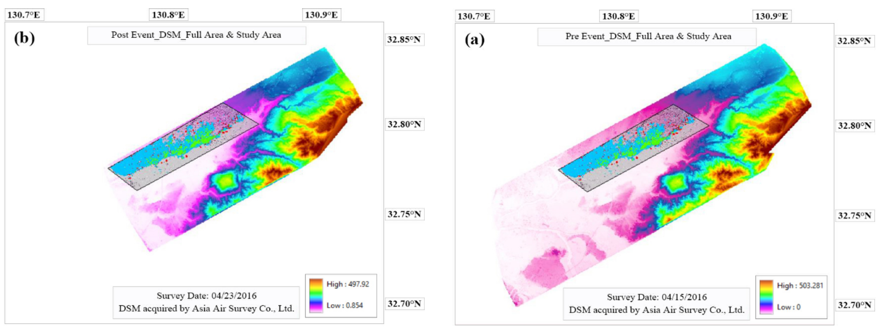
On 14 April 2016, an earthquake with a magnitude of 6.2 Mw hit the Kumamoto Prefecture, Japan. The epicenter of the foreshock and main shock was located at the Hinagu and Futugawa fault, respectively. The epicenter of foreshock was reported 12.0 km beneath Mount Kinpo that is located in the northwest of Kumamoto city center. While this was thought to be the main shock, on 16 April another earthquake with a magnitude of 7.0 Mw struck the region. The epicenter of this event was located under Higashi Ward of Kumamoto in the Kyushu Region in southwest Japan. The first shock was known as foreshock and the second as the main shock. However, most of the damage was in the eastern suburbs of Kumamoto in Mashiki. Because of this earthquake, 55 people died and more than 3000 people injured and many people became homeless. The collapse of about 8700 structures and severe damage to more than 35,000 buildings and numerous landslides across the mountains of Kyushu were other effect of this earthquake. Numerous studies have been conducted to assess the damage caused by this event, some of which were mentioned above. In this study, the combination of SAR and LIDAR data has been used for this purpose [5,8,12,18]. The location of pre- and post-event LIDAR data and the study area used in this research are illustrated in Figure 1 and Figure 2. In addition, registration date and other details of SAR and LIDAR images are shown in

Table 1. Registration date and other details of synthetic aperture radar (SAR) and LIDAR data.

SAR
Type	Date	Polarization	Spatial Resolution	Path Direction	Mode
Sentinel-1	3 March 2016	VV	20 m	D	Interferometric Wide
Sentinel-1	20 April 2016	VV	20 m	D	Interferometric Wide
Sentinel-1	27 June 2016	VV	20 m	D	Interferometric Wide
LIDAR
Collection Platform	Date	Data Provider		Area	Point Density
Airborne LIDAR	15 April 2016	Asia Air Survey Co., Ltd.		151.56 km2	2.94 pts/m2
Airborne LIDAR	23 April 2016	Asia Air Survey Co., Ltd.		95.85 km2	4.47 pts/m2

.

3. Methodology

In this study, three most common methods of damage assessment including elevation difference, coherence difference and texture difference have been used. In addition, machine-learning algorithms including RDF and SVM have been used to classify the information obtained from these methods. By using these methods in analyzing LIDAR and SAR images, valuable information can be obtained. Moreover, three computer programs including ENVI v.5.3, ArcGIS v.10.7.1 and XLSTAT v.2020 were used for buildings damage assessment. ENVI and ArcGIS, which are powerful tools for analyzing maps and other geographic information, were used to analyze SAR and LIDAR data. In addition, XLSTAT, which is an efficient tool for statistical data analysis, was used for machine learning.

3.1. Coherence

The coherence method has been used for damage assessment in several studies with successful results [1,13,22]. One of its applications is to measure the deformation and displacement of plates caused by earthquakes. In this method, the coherence extracted from the images before and after the event is subtracted. If the obtained result has a high value, it can be a reason for the destruction in the area. A simple or normalized difference method can be used to calculate the CD before and after the event.

$$CD={\mathsf{\gamma }}_{\mathrm{pre}}-{\mathsf{\gamma }}_{\mathrm{co}} or \widehat{CD}=\frac{{\mathsf{\gamma }}_{\mathrm{pre}}-{\mathsf{\gamma }}_{\mathrm{co}}}{{\mathsf{\gamma }}_{\mathrm{pre}}+{\mathsf{\gamma }}_{\mathrm{co}}}$$

(1)

where γ_pre and γ_co are pre- and co-event coherence images, respectively [1].

3.2. Texture Analysis

The textural properties of the areas can change over time due to natural or man-made events. These factors can affect the texture of the images in a natural or man-made event. By using the TD in the images before and after the event, different levels of damage can be identified. This method is used to classify land cover and assess the damage and other applications [23,24]. The seven second-order texture including Mean, Variance, Homogeneity, Dissimilarity, Contrast, Entropy and Correlation features were used in this study. The abovementioned features in the five window sizes (3 × 3, 5 × 5, 7 × 7, 9 × 9, 11 × 11) in the DSM images pre- and post-event were calculated separately and then the value obtained in the two images was subtracted.

Gray-level co-occurrence matrix (GLCM) is a statistical method for evaluating texture that considers the spatial relations between pixels. In order to calculate the second-order statistics, the pixel values of the image must first be converted to GLCM (Figure 3).

Mean (GLCM): The mean is applied to measure the average gray-level in the specific window on GLCM showing the location of distribution [24,25].

$${{\displaystyle \sum }}_{\mathrm{i},\mathrm{j}=0}^{\mathrm{N}-1}\mathrm{p}(\mathrm{i},\mathrm{j}).$$

(2)

Variance (GLCM): The variance is used to measure the gray-level variance and it is a measure of heterogeneity feature. It shows the condition of spreading the data around the mean [25].

$${{\displaystyle \sum }}_{\mathrm{i},\mathrm{j}=0}^{\mathrm{N}-1}{\mathrm{p}}_{\mathrm{i},\mathrm{j}}{{(\mathrm{i}-\mathsf{\mu }}_{\mathrm{i}})}^2.$$

(3)

Homogeneity (GLCM): The homogeneity calculates the number of homogeneous pixel values in a selected window in an image. If an image is homogeneous, a co-occurrence matrix will be formed with a combination of upper and lower values of P[i,j]. Otherwise a matrix with uniform values is created [24,25].

$${{\displaystyle \sum }}_{\mathrm{i}}{{\displaystyle \sum }}_{\mathrm{j}}\frac{1}{1+\left(\mathrm{i}-\mathrm{j}\right)}\mathrm{p}(\mathrm{i},\mathrm{j}).$$

(4)

Contrast (GLCM): The contrast GLCM feature indicates the local difference of pixel values in neighboring pixels. If the values of local variation are high, the p(i, j) will be concentrated away from the basic diagonal and the amount of contrast will be greater. [24,25].

$${{\displaystyle \sum }}_{\mathrm{n}=0}^{\mathrm{N}-1}{\mathrm{n}}^2\{{{\displaystyle \sum }}_{\mathrm{i}=1}^{\mathrm{N}}{{\displaystyle \sum }}_{\mathrm{j}=1}^{\mathrm{N}}\mathrm{p}(\mathrm{i},\mathrm{j})\}.$$

(5)

Dissimilarity (GLCM): The dissimilarity GLCM is dissimilar to variance and similar to the contrast [24,26].

$${{\displaystyle \sum }}_{\mathrm{n}=0}^{\mathrm{N}-1}\mathrm{n}\{{{\displaystyle \sum }}_{\mathrm{i}=1}^{\mathrm{N}}{{\displaystyle \sum }}_{\mathrm{j}=1}^{\mathrm{N}}\mathrm{p}(\mathrm{i},\mathrm{j})\}.$$

(6)

Entropy (GLCM): The entropy GLCM feature indicates the content of the information. If all entries in P [i, j] are of the same size, the entropy value will be higher and if the entries do not have equal values, the entropy value will be lower. [24,25,27].

$$-{{\displaystyle \sum }}_{\mathrm{i}}{{\displaystyle \sum }}_{\mathrm{j}}\mathrm{p}\left(\mathrm{i},\mathrm{j}\right)\log \left(\right(\mathrm{i},\mathrm{j}\left)\right).$$

(7)

Correlation (GLCM): The correlation GLCM shows the scale of image linearity. If an image has a significant linear structure, its value will be high [25].

$$\frac{{{\displaystyle \sum }}_{\mathrm{i}}{{\displaystyle \sum }}_{\mathrm{j}}\left(\mathrm{ij}\right)\mathrm{p}\left(\left(\mathrm{i},\mathrm{j}\right)\right){-\mathsf{\mu }}_{\mathrm{x}}{\mathsf{\mu }}_{\mathrm{y}}}{{\mathsf{\sigma }}_{\mathrm{x}}{\mathsf{\sigma }}_{\mathrm{y}}}.$$

(8)

3.3. Machine Learning

Machine learning is a computer tool that, by using the algorithms developed in it, can learn the numerical and visual patterns in data and images and use it to predict and categorize new data. The main part of machine learning is the training data in which the algorithms receive two types of data from the user. The first data is the input (extracted data of analysis) and the second is the output (rate of damages data, extracted from field survey). They learn the patterns and make predictions about new data. Today, machine learning is used in medical sciences, robotics, damage assessment and so forth. [14,16,28]. Conventional algorithms in this system include random forest (RDF), the support vector machine (SVM) and K-nearest neighbor (KNN). In this study, we used RDF and SVM.

3.3.1. Random Forest (RDF)

A random forest algorithm consists of a group of decision trees, each of which depends on a random vector and the same distribution of all forest trees. In addition, the amount of error in the forest depends on the power of each tree and the connection between them. This algorithm is of the supervised type that generates the forest algorithm randomly. RDF uses several decision trees to create accurate predictions. Classification and regression are the main applications of this algorithm. Any decision tree can easily work with complex data and make decisions from it [29,30]. In the regression problem, the result is the average of all trees (Equation (10)) and in the classification problem, we obtain the final answer by voting between the trees (Figure 4).

$$F\left(X\right)=\frac{1}{B}{\displaystyle {{\displaystyle \sum }}_{b=1}^B}{T}_b\left(x\right).$$

(9)

3.3.2. Support Vector Machine (SVM)

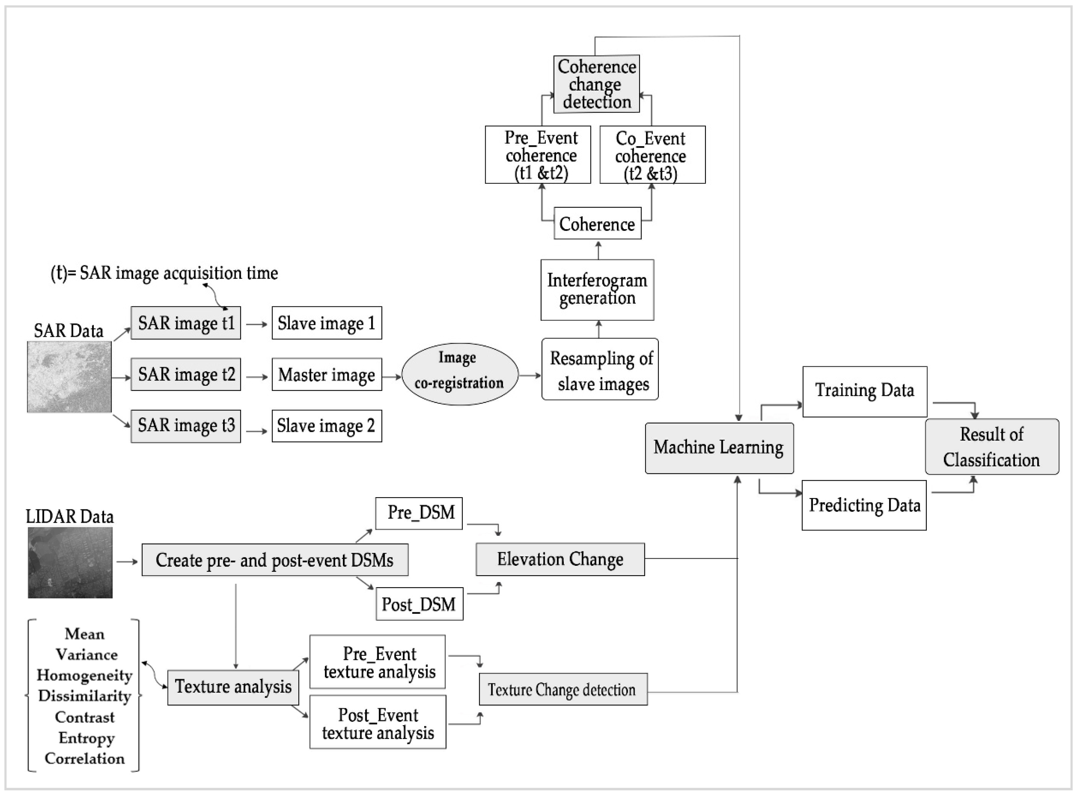
SVM is a non-parametric statistical monitoring method used for classification and regression. The SVM algorithm can be used wherever there is a need to identify patterns or classify objects in specific classes. In this method, each data sample is represented as a point in the n-dimensional space in the data scatter diagram. The value of each feature related to the data determines one of the point coordinate parameters in the graph. The SVM classification base is a linear classification of data and in linear segmentation of data, a more reliable line is chosen. [16,31]. Figure 4 makes it easier to understand. As you can see, the H3 does not divide the two batches. H1 does this with a small margin and H2 separates the two categories with a maximum margin. Figure 5 shows the flowchart of methods used for damage assessment using machine-learning algorithms.

$$\mathrm{D}=\left\{{(\mathrm{X}}_{\mathrm{i}}, {\mathrm{Y}}_{\mathrm{i}}{\left)\right|\mathrm{X}}_{\mathrm{i}}\in {\mathrm{R}}^{\mathrm{p}}, {\mathrm{Y}}_{\mathrm{i}}\in \{-1,1\right\}{\}}_{\mathrm{i}}^{\mathrm{n}}=1$$

(10)

3.4. Damage Classification

In this study, we considered seven damage rates based on the Architectural Institute of Japan (AIJ) including D0, D1, D2, D3, D4, D5 and D6, which due to the limited ability of the methods, the number of rates has been reduced to 3 and 4 levels. In the first case, four damage rates (4DR), including D0 and D1 (Negligible to slight damages), D2 and D3 (Moderate damages), D4 and D5 (Very Heavy damage) and D6 (Collapsed buildings) and in the second case, three damage rates (3DR), including D0 and D1 (Negligible to slight damages), D2, D3 and D4 (Moderate to Heavy damages) and D5 and D6 (Collapsed buildings) have been considered. It should be noted that the truth data (damage rate of structures) used in this study were extracted from the research of Goto et al. [32]. The total number of buildings studied in two cases was 18,445 buildings, which are shown separately in

Table 2. The number of structures in the study area and the number of structures intended for training and prediction in 3 and 4 rate of damages.

4DR
Group Name	Damage Level	Number of Total Buildings	Number of Training Buildings	Number of Prediction Buildings
D0, D1	Negligible to Slight	2634	700	1934
D2, D3	Moderate	13,007	700	12,307
D4, D5	Very heavy	1676	700	973
D6	Collapsed	1128	700	428
3DR
Group Name	Damage Level	Number of Total Buildings	Number of Training Buildings	Number of Prediction Buildings
D0, D1	Negligible to Slight	2634	1000	1634
D2, D3, D4	Moderate to Heavy	14,683	1000	13,683
D5, D6	Very heavy to Collapsed	1128	1000	128

.

3.5. Training and Prediction Dataset

In the machine learning method, part of the data must be allocated for algorithm training. If more training data is given to the algorithm, its analysis will be better and it can have more accurate estimation results. But in this study, due to the low number of buildings in group D6 (1128 buildings), we had to choose the number of data in proportion to this group. Therefore, fewer buildings were selected to the algorithm training, which in turn reduces the accuracy of the assessment. The number of selected buildings for training and estimation in 3DR and 4DR cases are shown in Table 2. Also, Figure 6 shows the position of buildings in 3DR mode.

4. Results

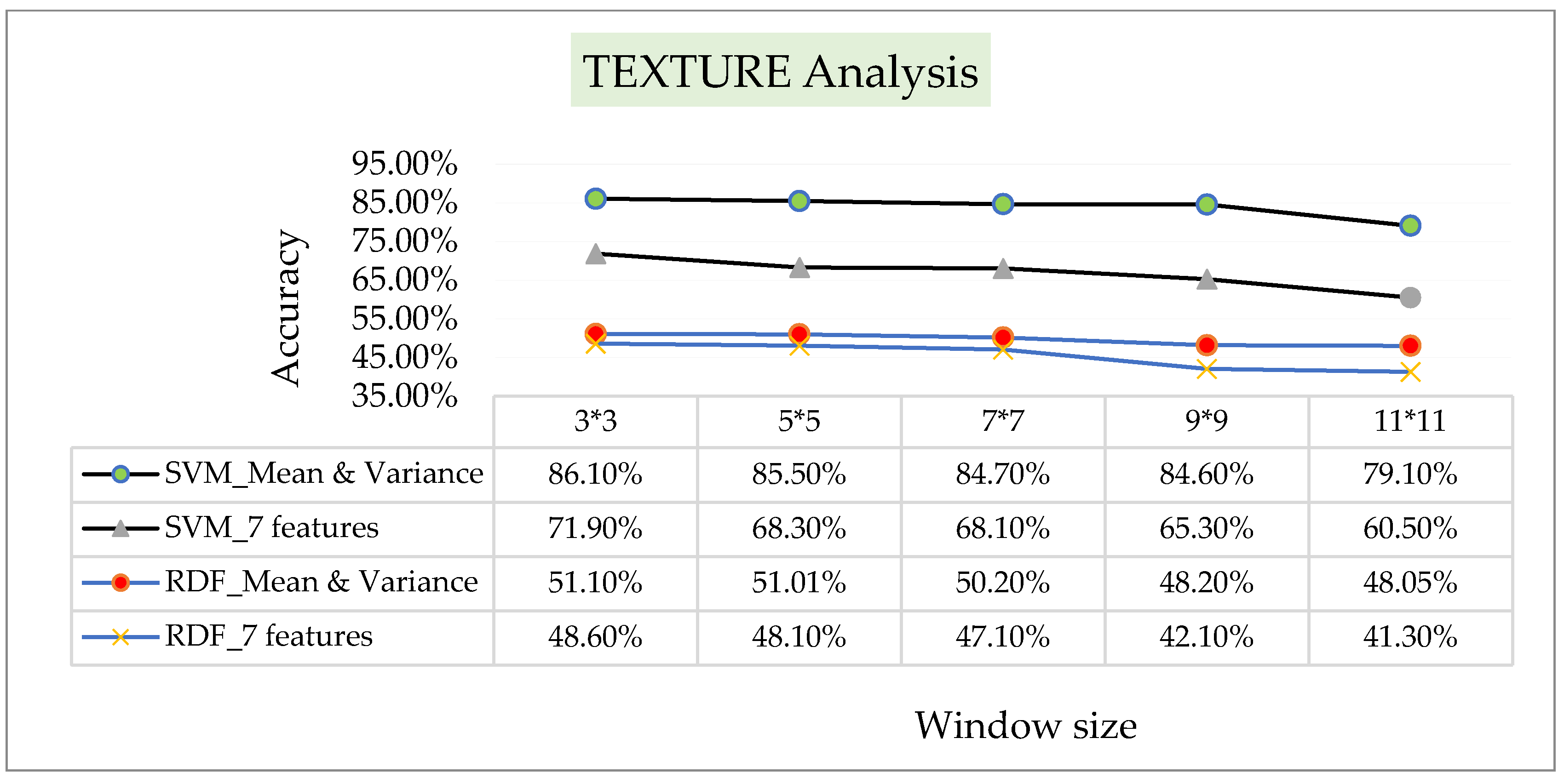
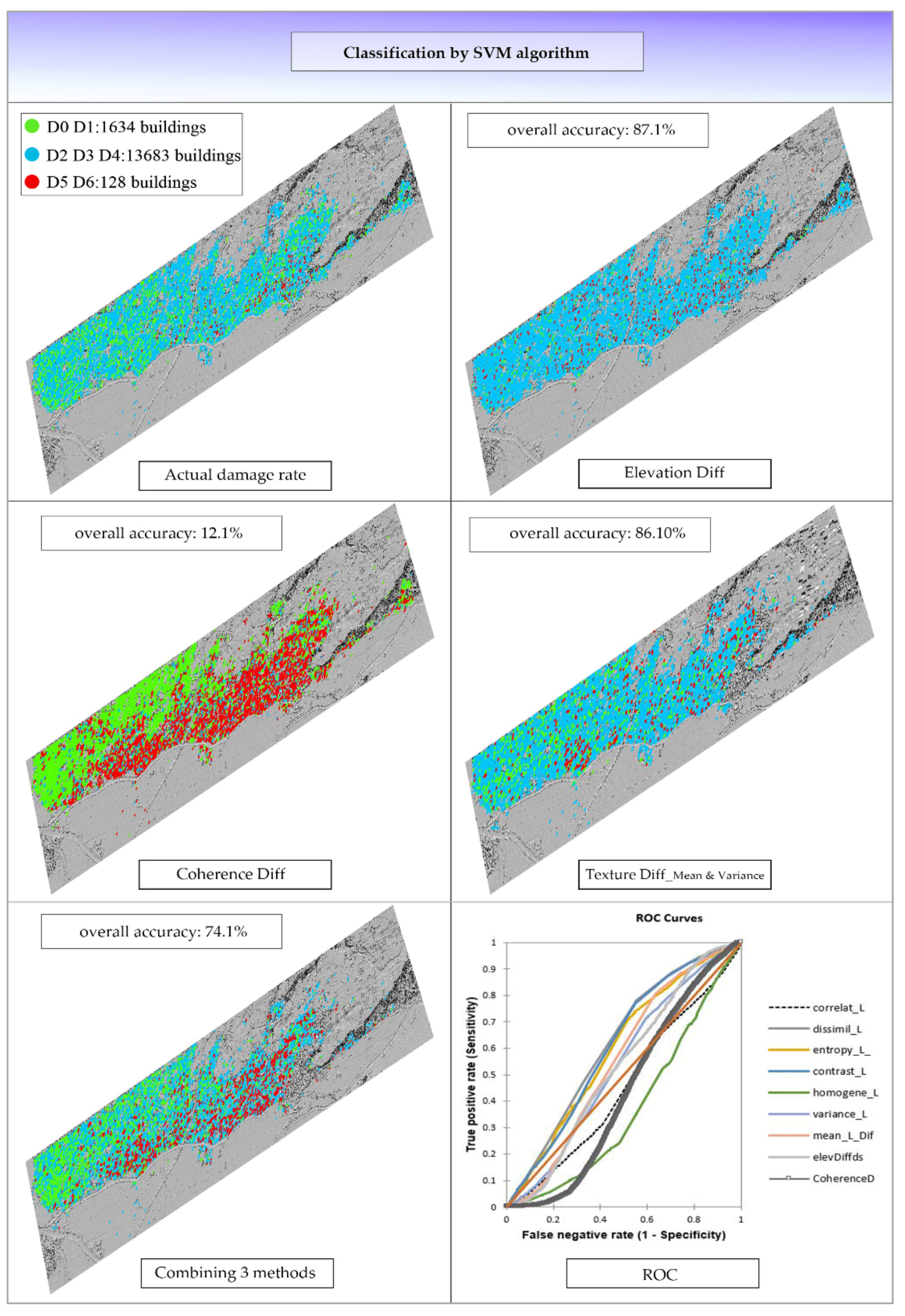
For better understanding of the effectiveness of ELD, TD and CD methods, each was first analyzed separately and then three methods were combined. Due to the variability of window size in texture analysis, this method was first examined in five window sizes. The results showed that 3 × 3 window size had the best performance (Figure 7), so we chose it as the final result of this method according to damage states explained in Figure 8. It should be noted that among the 7 parameters of this method, mean and variance parameters provided the highest overall accuracy. In the next stage of analysis, the results of DSMs were extracted, which showed that this method has an ability to assess the damage so that it provided an overall accuracy of 78.1% for 4DR state (Figure 9). In addition, in 3DR state, the overall accuracy was 87.1%. In damage detection using remote sensing images that are viewed vertically, since direct information about the damage of columns, walls and internal components of the building is not available, the roof of the structure plays a key role in classifying the damage. In some cases, in moderately damaged buildings, residents may cover the roof of the building with a blue plastic tarp to prevent water penetration. This makes it difficult to detect moderate damage in blue tarp-covered ceilings in post-event images [15]. Also, by considering other factors that reduce the accuracy of the results, such as the horizontal difference in the images caused by landslides and the great imbalance in the three groups of damage, it can be said that the evaluation provided an acceptable accuracy) Figure 10). According to the experimental results of this study, if the number of response variables (in this study: the number of damage rates) is increased, the amount of training data should be increased accordingly. Otherwise, the algorithm will not have the correct analysis and estimation. In this study, due to the low number of buildings with a damage rate of D2 to D6, it was not possible to increase the number of training data. If the number of training data increased, there would be no data to estimate. For example, the number of structures in the collapsed group was 1128 structures. From these, 1000 structures were used for machine training and 128 structures for predicting. Basically, the number of training data in each group should be the same, so in the other groups, the number of this data was selected in proportion to the D6 group. Despite this fact, most of the time, after earthquakes or other catastrophes, there is no balance in the data and this problem must be solved in another way. On the other hand, having a large number of structures in the study area and multiplicity of variables reduce the efficiency of algorithms and the accuracy of the results. To reduce the impact of these problems, better results can be obtained by dividing large areas into several small areas and by performing several separate analyses.

In the following part of the study, the pre-processed coherence data of pre- and post-event were subtracted from each other. After using machine learning algorithms, despite the significant advantage of this method, which has been emphasized in various researches, it resulted in very low accuracy. The results of CD method showed that this method is not able to detect minor to moderate damages. For example, in 3DR case, by examining the results, it was found that the algorithm classified the majority of D2 data as underestimation in the almost intact group (Negligible to Slight damage) and categorized the majority of D4 data as overestimation in the Collapsed group. In addition, group D3 is divided between groups depending on the extent of damages.

In the last part of the study, the values of the above three methods were combined. The results showed that the TD and CD, despite their good capabilities, led to poorer results in this evaluation in combination with the ELD (

Table 3. Producer accuracy, user accuracy and overall accuracy [34] for RDF and SVM classifiers by considering the combination method (3DR).

Combination of 3 Methods
Type of Accuracy	SVM (%)	RDF (%)
Producer Accuracy (D0, D1)	26.13	14.44
Producer Accuracy (D2, D3, D4)	55.09	94.85
Producer Accuracy (D5, D6)	91.19	5.1
User Accuracy (D0, D1)	35.01	79.06
User Accuracy (D2, D3, D4)	78.79	34.52
User Accuracy (D5, D6)	61.17	66.40
Overall Accuracy (3 category)	74.1	39.2

).

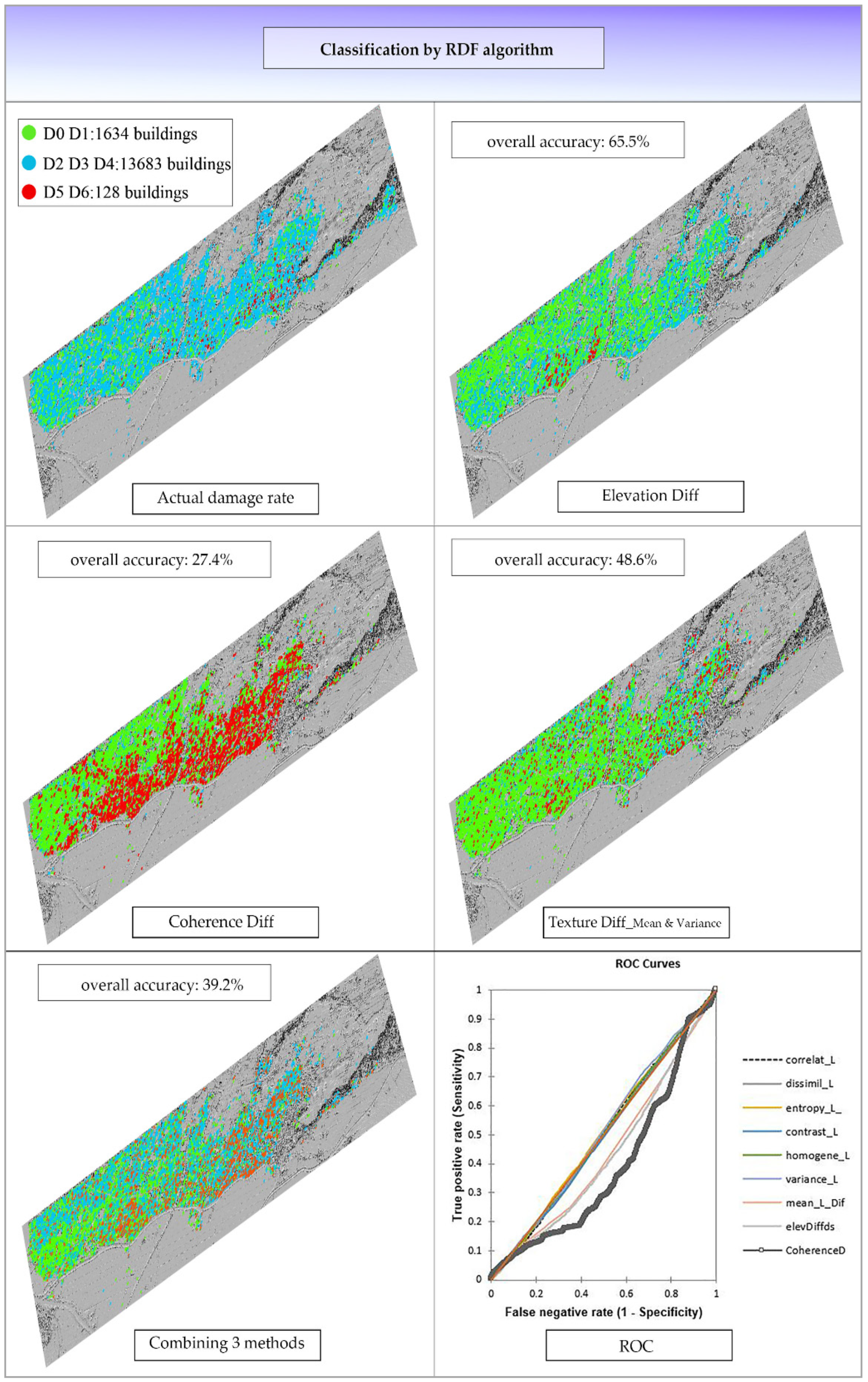
Examining the results of this study and various researches were done with SVM and RDF algorithms; it can be experimentally concluded that the SVM algorithm using LIDAR images leads to higher accuracy than the RDF algorithm. In addition, the performance of the RDF algorithm in evaluating SAR images in compared to the SVM algorithm is better (Figure 11). Although the RDF is known as a strong classifier due to its “bagged decision tree” nature, which can split data on a subset of features, as mentioned above, the main reason for the low overall accuracy in RDF were the increase in the number of damage rates (response variables) and lack of enough training data. In general, we can say that, when we use several different datasets its performance and accuracy may reduce [35]. On the other hand, SVM provides better results when multiple datasets and smaller training set is available [35].

Table 4. Some examples of research done with RDF and SVM algorithms using LIDAR images.

No	Research	Type of Data	Algorithm	Accuracy	Event
1	Moya et al. [5]	LIDAR	SVM	92%	Kumamoto earthquake
2	Rastiveis et al. [37]	LIDAR	SVM	91.59%	Haiti earthquake
3	Axel and Aardt [38]	LIDAR	SVM	78.90%	Haiti earthquake
4	Torres et al. [39]	LIDAR	SVM	78.8%	Lorca earthquake
5	Mehdi Rezaeian [40]	LIDAR	SVM	80%	Kobe earthquake
6	Singh et al. [35]	Landsat, ALOS and LIDAR	SVM	98%	Cambodia forests
			RDF	66%

shows some previous studies in which SVM and RDF algorithms were used for damage/land classification. Figure 12 and Figure 13 also show the estimated results, of the SVM and RDF algorithms.

5. Discussion

The ELD method showed that the calculation of changes in the height of buildings in pre- and post-event LIDAR images provides valuable information. Through this method, a quick and acceptable assessment can be made after earthquakes and other disasters. TD is another method that can be applied for both SAR and LIDAR images. In this study, it was used to assess changes in textural features in pre- and post-event LIDAR images (in five window sizes). The results showed that this method has a good ability to assess the damage of buildings. Despite several advantages of CD method, poor results were obtained. It can be said that one of the main reasons of very low overall accuracy of this method is the overestimation or underestimation evaluation of the algorithms, which eliminates the low to moderate rate of damage from the results. Regarding the fusion of the above three methods together or in fact, the combination of two sensors data, it can be said that this method could not improve the overall accuracy of the evaluation. The results of SVM algorithm demonstrated that this algorithm could provide an acceptable estimate using LIDAR images and by considering ELD and TD methods. In the present study, the RDF algorithm provided low accuracy. The main reason is that this algorithm, by increasing the response variables (in this study: the number of degrees of damage), requires more training data for accurate analysis and estimation.

6. Conclusions

In this study, a combination of SAR and LIDAR images was used for evaluation. The CD parameter in pre- and co-event SAR images and the TD (in five window sizes) and the ELD parameters in pre- and post-event LIDAR images were analyzed. To classify and predict the results, machine learning-based algorithms, including RDF and SVM were used. In the first step, the LIDAR images were preprocessed and pre- and post-event DSMs were extracted. Then, the variation between the two images was calculated by simple differentiation. In the second step, the seven second-order texture parameters (Mean, Variance, Homogeneity, Dissimilarity, Contrast, Entropy and Correlation) in 5 window sizes (3 × 3, 5 × 5, 7 × 7, 9 × 9, 11 × 11) were calculated separately for pre- and post-event images. Then, the differences of the extracted parameters in the two images were computed. In the third step, after analyzing the SAR data and creating coherence images, the difference between both images was calculated. In order to estimate and categorize the results, machine-learning algorithms including RDF and SVM were used. Part of the data was allocated for algorithms training and the rest of the data was used to predict the rate of damages. This study was performed in two cases: in the first case, 3 damage rates and in the second case, 4 damage rates were considered. The SVM algorithm using the ELD parameter and considering three damage rates provided an overall accuracy of about 87.1%. In addition, in 4 damage rates, the overall accuracy was about 78.1%. The results showed that methods based on LIDAR images are more efficient. Regarding the methods used to analyze these images, we conclude that:

• In the future, the LED method can be a good alternative to field research, which is very time consuming and costly.
• Among seven texture properties mentioned in the previous sections, mean and variance played a more effective role in the results. According to the results from this method, it can be considered as a complement to other methods. In a separate experiment with two damage rates, the overall accuracy of this method increased about 10%.

The CD method based on SAR data provided poor results in identifying the three damage rates. In evaluating the two groups of damage, including intact buildings (D0, D1, D2) and collapsed group (D3, D4, D5, D6), the overall accuracy of this method increased to about 60%. Another factor that could increase the accuracy of this method about 8% was the division of study areas, which made it easier to make algorithms decisions. In general, it can be said that this method cannot still be replaced by field study because it has low ability to evaluate buildings with moderate to low damage.

Regarding the current capability of machine learning algorithms, for future work, it is recommended that building damage assessments be performed in several separate sections with less data, rather than an integrated analysis for a large area. In addition, the effects of landslides on reducing the accuracy of the results can be investigated.

References

1. Karimzadeh, S.; Matsuoka, M.; Miyajima, M.; Adriano, B.; Fallahi, A.; Karashi, J. Sequential SAR coherence method for the monitoring of buildings in Sarpole-Zahab, Iran. Remote Sens. 2018, 10, 1255. [Google Scholar] [CrossRef] [Green Version]
2. Matsuoka, M.; Yamazaki, F. Use of satellite SAR intensity imagery for detecting building areas damaged due to earthquakes. Earthq. Spectra 2004, 20, 975–994. [Google Scholar] [CrossRef]
3. Matsuoka, M.; Yamazaki, F. Building damage mapping of the 2003 Bam, Iran, earthquake using Envisat/ASAR intensity imagery. Earthq. Spectra 2005, 21, 285–294. [Google Scholar] [CrossRef]
4. Karimzadeh, S.; Matsuoka, M. Building damage characterization for the 2016 Amatrice earthquake using ascending–descending COSMO-SkyMed data and topographic position index. IEEE. J. Sel. Top Appl. Earth. Obs. Remote Sens. 2016, 11, 2668–2682. [Google Scholar] [CrossRef]
5. Moya, L.; Yamazaki, F.; Liu, W.; Yamada, M. Detection of collapsed buildings from lidar data due to the 2016 Kumamoto earthquake in Japan. Nat. Hazards Earth Syst. Sci. 2018, 18, 65–78. [Google Scholar] [CrossRef] [Green Version]
6. Bai, Y.; Adriano, B.; Mas, E.; Koshimura, S. Machine learning based building damage mapping from the ALOS-2/PALSAR-2 SAR imagery: Case study of 2016 Kumamoto earthquake. J. Disaster Res. 2017, 12, 646–655. [Google Scholar] [CrossRef]
7. Jaboyedoff, M.; Oppikofer, T.; Abellán, A.; Derron, M.-H.; Loye, A.; Metzger, R.; Pedrazzini, A. Use of LIDAR in landslide investigations: A review. Nat. Hazards 2012, 61, 5–28. [Google Scholar] [CrossRef] [Green Version]
8. Liu, W.; Yamazaki, F.; Maruyama, Y. Detection of earthquake-induced landslides during the 2018 Kumamoto earthquake using multitemporal airborne Lidar data. Remote Sens. 2019, 11, 2292. [Google Scholar] [CrossRef] [Green Version]
9. Plank, S. Rapid damage assessment by means of multi-temporal SAR—A comprehensive review and outlook to Sentinel-1. Remote Sens. 2014, 6, 4870–4906. [Google Scholar] [CrossRef] [Green Version]
10. Sharma, M.; Garg, R.; Badenko, V.; Fedotov, A.; Min, L.; Yao, A. Potential of airborne LiDAR data for terrain parameters extraction. Quat. Int. 2020, in press. [Google Scholar] [CrossRef]
11. Karimzadeh, S.; Matsuoka, M. A weighted overlay method for liquefaction-related urban damage detection: A case study of the 6 September 2018 Hokkaido Eastern Iburi earthquake, Japan. Geosciences 2018, 8, 487. [Google Scholar] [CrossRef] [Green Version]
12. Muller, J.R.; Harding, D.J. Using LIDAR surface deformation mapping to constrain earthquake magnitudes on the Seattle fault in Washington State, USA. 2007 Urban Remote Sens. Jt. Event 2007, 7, 1–7. [Google Scholar] [CrossRef]
13. Yamazaki, F.; Liu, W. Remote sensing technologies for post-earthquake damage assessment: A case study on the 2016 Kumamoto earthquake. In Proceedings of the 6th ASIA Conference on Earthquake Engineering, Cebu City, Philippines, 22–24 September 2016; p. KN4. [Google Scholar]
14. Hajeb, M.; Karimzadeh, S.; Fallahi, A. Seismic damage assessment in Sarpole-Zahab town (Iran) using synthetic aperture radar (SAR) images and texture analysis. Nat. Hazards 2020, 103, 1–20. [Google Scholar] [CrossRef]
15. Miura, H.; Aridome, T.; Matsuoka, M. Deep learning-based identification of collapsed, non-collapsed and blue tarp-covered buildings from post-disaster aerial images. Remote Sens. 2020, 12, 1924. [Google Scholar] [CrossRef]
16. Karimzadeh, S.; Matsuoka, M.; Kuang, J.; Ge, L. Spatial prediction of aftershocks triggered by a major earthquake: A binary machine learning perspective. ISPRS Int. J. Geo-Inf. 2019, 8, 462. [Google Scholar] [CrossRef] [Green Version]
17. Bai, Y.; Adriano, B.; Mas, E.; Koshimura, S. Building damage assessment in the 2015 Gorkha, Nepal, earthquake using only post-event dual polarization synthetic aperture radar imagery. Earthq. Spectra 2017, 33, 185–195. [Google Scholar] [CrossRef]
18. Yamazaki, F.; Sagawa, Y.; Liu, W. Extraction of landslides in the 2016 Kumamoto earthquake using multi-temporal Lidar data. In Earth Resources and Environmental Remote Sensing/GIS Applications IX, Proceedings of the SPIE Remote Sensing, Berlin, Germany, 11–13 September 2018; SPIE: Bellingham, WA, USA, 2018; Volume 10790, p. 107900H. [Google Scholar] [CrossRef]
19. Google Earth. Available online: https://earth.google.com/web/search/Kumamoto,+Japan (accessed on 19 July 2020).
20. Pre-Kumamoto Earthquake (16 April 2016) Rupture Lidar Scan. OpenTopography, High-Resolution Topography Data and Tools. Available online: https://portal.opentopography.org/datasetMetadata?otCollectionID=OT.052018.2444.2 (accessed on 12 July 2020).
21. Post-Kumamoto Earthquake (16 April 2016) Rupture Lidar Scan. OpenTopography, High-Resolution Topography Data and Tools. Available online: https://portal.opentopography.org/datasetMetadata?otCollectionID=OT.052018.2444.1 (accessed on 12 July 2020).
22. Tamkuan, N.; Nagai, M. Sentinel-1A analysis for damage assessment: A case study of Kumamoto earthquake in 2016. MATTER Int. J. Sci. Technol. 2019, 5, 23–35. [Google Scholar] [CrossRef] [Green Version]
23. Whelley, P.; Glaze, L.S.; Calder, E.S.; Harding, D.J. LiDAR-derived surface roughness texture mapping: Application to Mount St. Helens Pumice Plain deposit analysis. IEEE. Trans. Geosci. Remote Sens. 2013, 52, 426–438. [Google Scholar] [CrossRef]
24. Gong, L.; Wang, C.; Wu, F.; Zhang, J.; Zhang, H.; Li, Q. Earthquake-induced building damage detection with post-event sub-meter VHR TerraSAR-X staring spotlight imagery. Remote Sens. 2016, 8, 887. [Google Scholar] [CrossRef] [Green Version]
25. Wood, E.M.; Pidgeon, A.M.; Radeloff, V.C.; Keuler, N.S. Image texture as a remotely sensed measure of vegetation structure. Remote Sens. Environ. 2012, 121, 516–526. [Google Scholar] [CrossRef]
26. Haralick, R.M.; Shanmugam, K.; Dinstein, I. Textural features for image classification. IEEE Trans. Syst. Man Cybern. 1973, 3, 610–621. [Google Scholar] [CrossRef] [Green Version]
27. Scalco, E.; Fiorino, C.; Cattaneo, G.M.; Sanguineti, G.; Rizzo, G. Texture analysis for the assessment of structural changes in parotid glands induced by radiotherapy. Radiother. Oncol. 2013, 109, 384–387. [Google Scholar] [CrossRef] [PubMed]
28. Santos, A.; Figueiredo, E.; Silva, M.; Sales, C.; Costa, J. Machine learning algorithms for damage detection: Kernel-based approaches. J. Sound Vib. 2016, 363, 584–599. [Google Scholar] [CrossRef]
29. Rodriguez-Galiano, V.; Chicaolmo, M.; Abarca-Hernández, F.; Atkinson, P.M.; Jeganathan, C. Random forest classification of Mediterranean land cover using multi-seasonal imagery and multi-seasonal texture. Remote Sens. Environ. 2012, 121, 93–107. [Google Scholar] [CrossRef]
30. Breiman, L. Random forests. Mach. Learn. 2001, 45, 5–32. [Google Scholar] [CrossRef] [Green Version]
31. Mountrakis, G.; Im, J.; Ogole, C. Support vector machines in remote sensing: A review. ISPRS J. Photogramm. Remote Sens. 2011, 66, 247–259. [Google Scholar] [CrossRef]
32. Goto, T.; Miura, H.; Mastuoka, M.; Mochizuki, K.; Koiwa, H. Building damage detection from optical images based on histogram equalization and texture analysis following the 2016 Kumamoto, Japan earthquake. In Proceedings of the International Symposium of Remote Sensing, Nagoya, Japan, 17–19 May 2017. [Google Scholar]
33. Okada, S.; Takai, N. Classifications of structural types and damage patterns of buildings for earthquake field investigation. J. Struct. Constr. Eng. (Trans. AIJ) 1999, 64, 65–72. [Google Scholar] [CrossRef] [Green Version]
34. Humboldt State University. Accuracy Metrics. Available online: http://gsp.humboldt.edu/OLM/Courses/GSP216Online/lesson6-2/metrics.html/ (accessed on 4 January 2019).
35. Singh, M.; Evans, D.; Chevance, J.-B.; Tan, B.S.; Wiggins, N.; Kong, L.; Sakhoeun, S. Evaluating remote sensing datasets and machine learning algorithms for mapping plantations and successional forests in Phnom Kulen National Park of Cambodia. PeerJ 2019, 7, e7841. [Google Scholar] [CrossRef]
36. XLstat, Data Analysis Solution. Available online: https://www.xlstat.com/en/solutions/features/roc-curves (accessed on 4 January 2020).
37. Rastiveis, H.; Eslamizade, F.; Hosseini-Zirdoo, E. Building damage assessment after earthquake using post-event LiDAR data. ISPRS Int. Arch. Photogramm. Remote Sens. Spat. Inf. Sci. 2015, 595–600. [Google Scholar] [CrossRef] [Green Version]
38. Axel, C.; van Aardt, J. Building damage assessment using airborne lidar. J. Appl. Remote Sens. 2017, 11, 1. [Google Scholar] [CrossRef] [Green Version]
39. Torres, Y.; Arranz-Justel, J.-J.; Gaspar-Escribano, J.M.; Gaspar-Escribano, J.M.; Martínez-Cuevas, S.; Benito, M.B.; Ojeda, J.C. Integration of LiDAR and multispectral images for rapid exposure and earthquake vulnerability estimation. Application in Lorca, Spain. Int. J. Appl. Earth Obs. Geoinf. 2019, 81, 161–175. [Google Scholar] [CrossRef] [Green Version]
40. Rezaeian, M. Assessment of Earthquake Damages by Image-Based Techniques. Ph.D. Thesis, Eidgenössischen Technischen Hochschule, Zurich, Switzerland, 2010. [Google Scholar]
Figure 1. The location of pre- and post-event light detection and ranging (LIDAR) data and the study area [19].
Applsci 10 08932 g001
Figure 2. Location of the pre-event (a) and post-event (b) DSMs and study area. DSMs acquired by Asia Air Survey Co., Ltd. (Tokyo, Japan) [20,21].
Applsci 10 08932 g002
Figure 3. An example of Gray Level Co-occurrence Matrix (GLCM).
Applsci 10 08932 g003
Figure 4. Classification process of random forest (RDF) in (left) and support vector machine (SVM) in (right).
Applsci 10 08932 g004
Figure 5. The flowchart of methods used for damage assessment using Machine Learning algorithms.
Applsci 10 08932 g005
Figure 6. Location of training (a) and prediction (b) dataset of the study area. Green points (intact buildings), Blue points (low to medium damage) and Red points (Collapsed buildings) (3DR).
Applsci 10 08932 g006
Figure 7. Texture analysis results considering 5 window sizes using RDF and SVM algorithms (3DR).
Applsci 10 08932 g007
Figure 8. The Architectural Institute of Japan scale (AIJ) [15,33].
Applsci 10 08932 g008
Figure 9. Prediction results of RDF and SVM algorithms by considering texture difference (TD) (Mean and Variance), elevation difference (ELD), coherence difference (CD) and Combination of three methods (4DR).
Applsci 10 08932 g009
Figure 10. The estimation results of the building conditions by SVM algorithm with considering 4 methods. The green spots represent the intact buildings, blue spots show low to moderate damage and the red spots represent the collapsed buildings. In addition, the Receiver’s Operating Characteristic (ROC) [36] curve (3DR) is shown.
Applsci 10 08932 g010
Figure 11. The estimation results of the building conditions by RDF algorithm by considering 4 methods. The green spots represent the intact buildings, blue spots show low to moderate damage and the red spots represent the collapsed buildings. In addition, the Receiver’s Operating Characteristic (ROC) [36] curve (3DR) is shown.
Applsci 10 08932 g011
Figure 12. Estimated results, of the SVM algorithm by considering 4 methods (3DR).
Applsci 10 08932 g012
Figure 13. Estimated results, of the RDF algorithm by considering 4 methods (3DR).
Applsci 10 08932 g013