Nonlinear Dynamic Analysis of Lifting Mechanism of an Electric Overhead Crane during Emergency Braking


Abstract
:1. Introduction
2. Dynamic Model
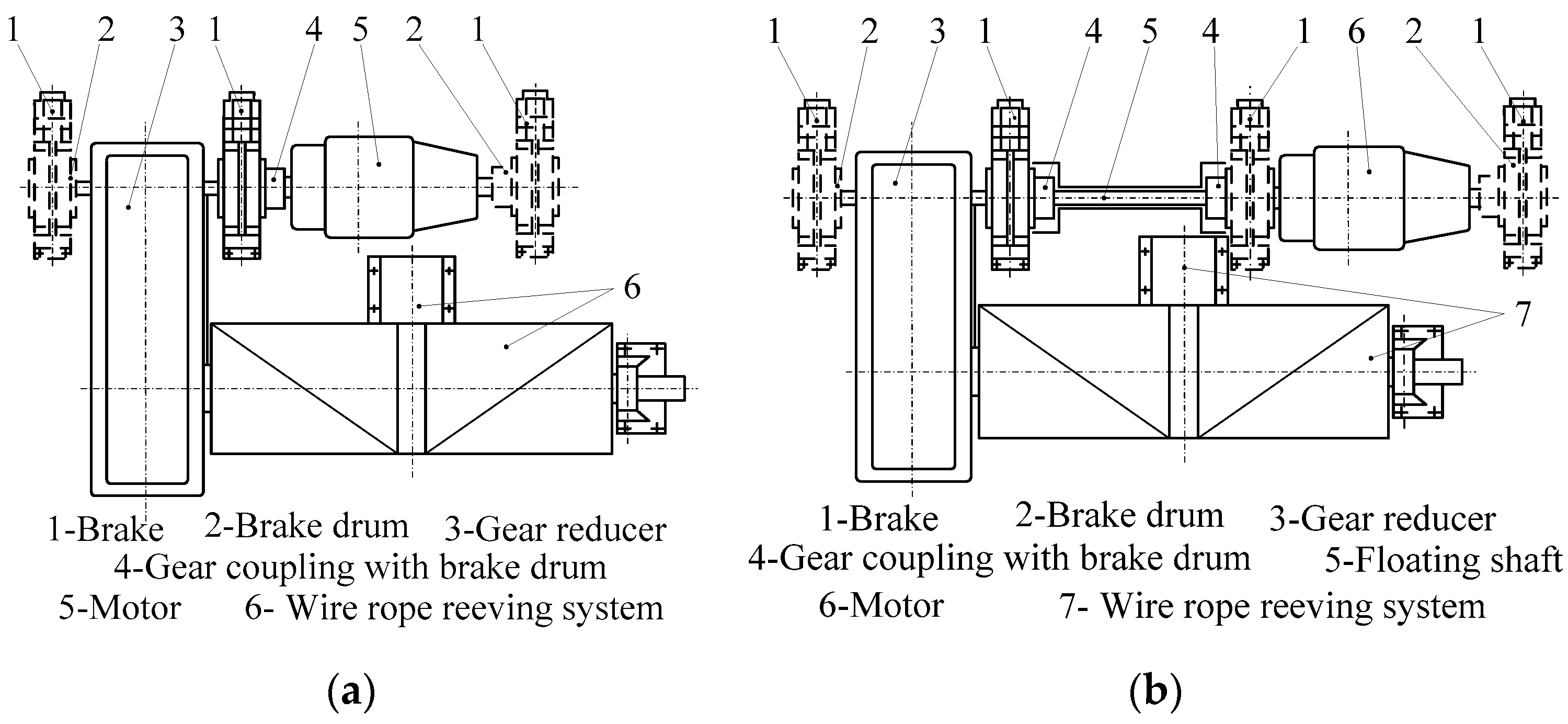
2.1. Physical Model and Assumption
- The two girders are treated as elastic Euler beams with the same small curvature, uniform damping and mass distributions.
- The wire rope is deemed to be a massless elastic body with a constant modulus of elasticity and viscous damping and can withstand only axial tension.
- The trolley frame, stators and rotors of motors, couplings, brake drums (or discs), the rope drums, gears, reducer housings, rope sheaves, steel wheels, and end carriages are considered rigid bodies. The payload (including the load handling device) is assumed to be a point mass.
- The clearances between transmission parts are negligible.
2.2. Energy of System
2.3. Virtual Work of Non-Conservative Forces
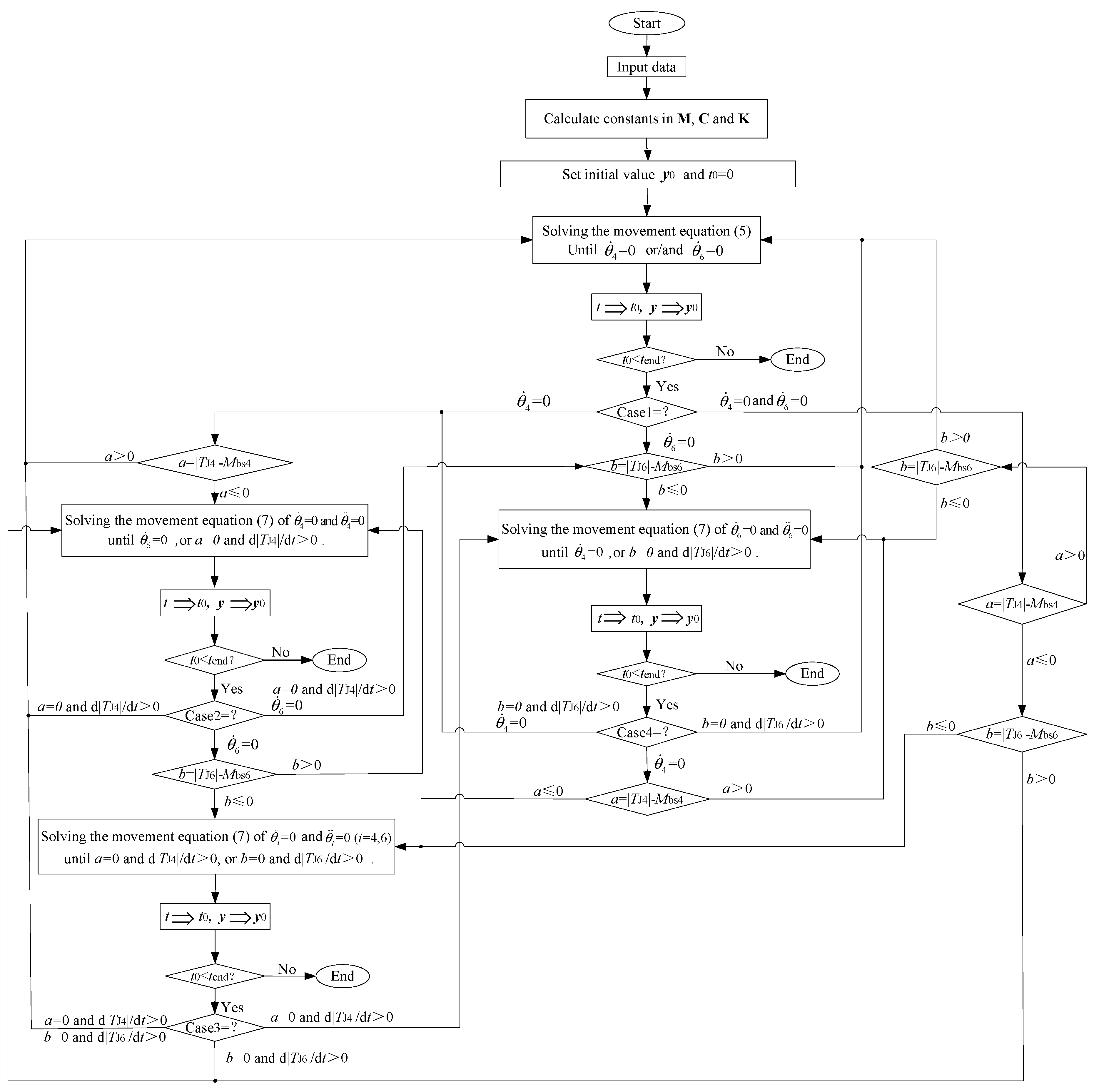
2.4. Equation of Motion and Simulation Algorithm
- (1)
- When component Ji is in the rotation state initially, needs to be checked at the end of each step of the numerical integration. If , then Jiis still in the rotation state; once , must be calculated ( is an algebraic sum of all torques acting on component Ji except braking torque ). If , component Ji starts to go into the non-rotation state; otherwise, component Ji will continue to rotate after this time instant when the direction of rotation of component Ji changes.
- (2)
- When component Ji is in the non-rotation state initially, needs to be calculated at the end of each step of the numerical integration. Once and , component Ji will start to go into the rotation state. Otherwise, component Ji will still be in the non-rotation state.
3. Simulation Parameters
4. Time Histories of Two Basic Scenarios
5. Discussions
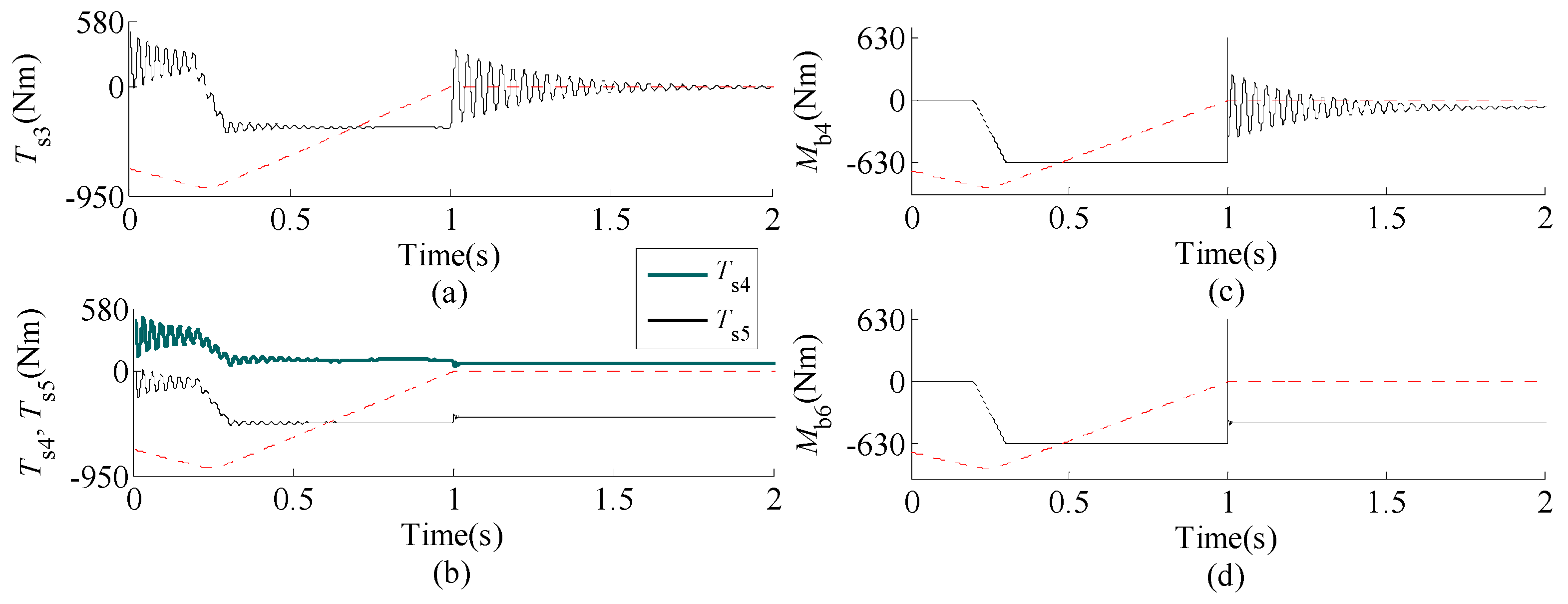
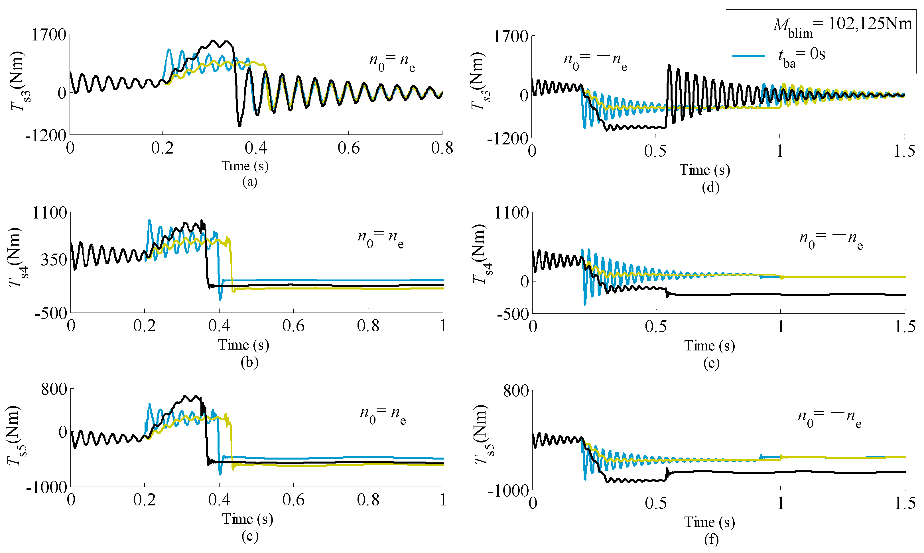
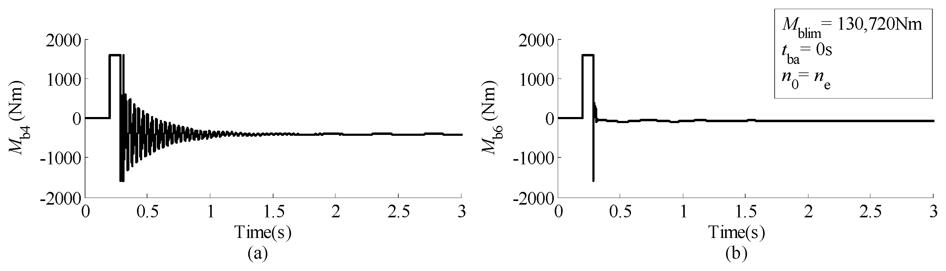
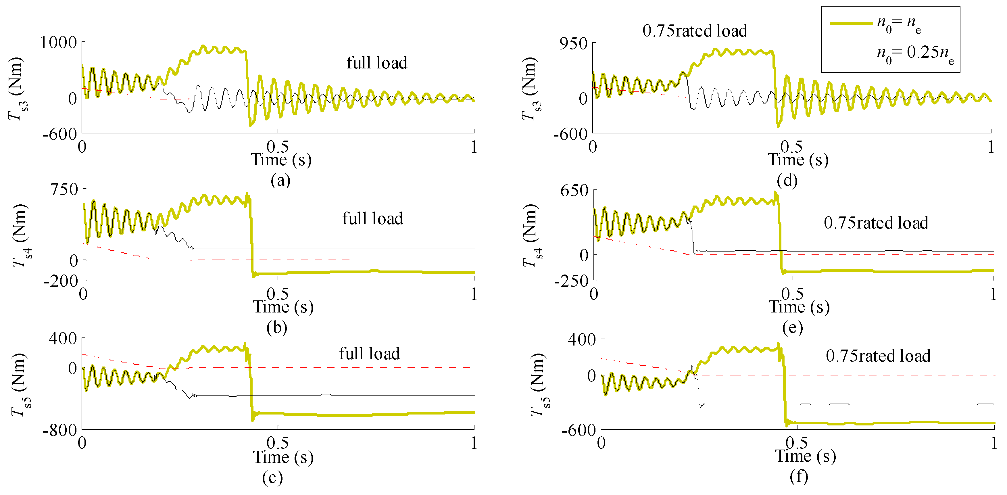
5.1. Time Histories of High-Speed Links
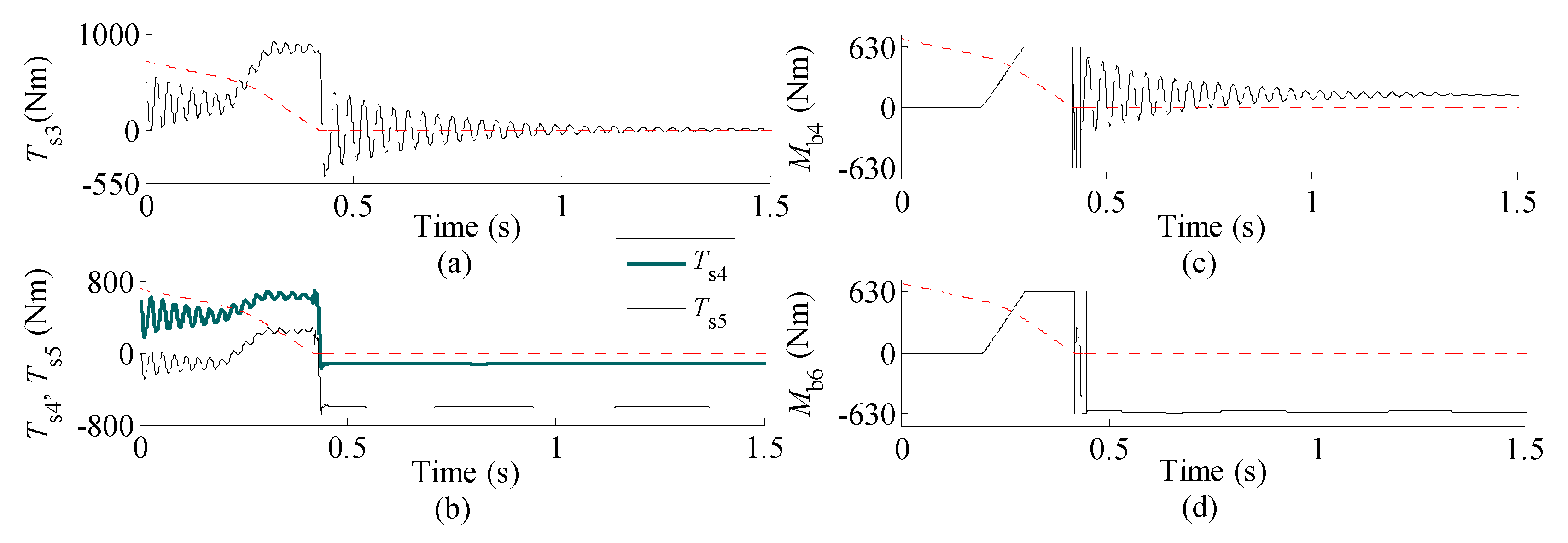
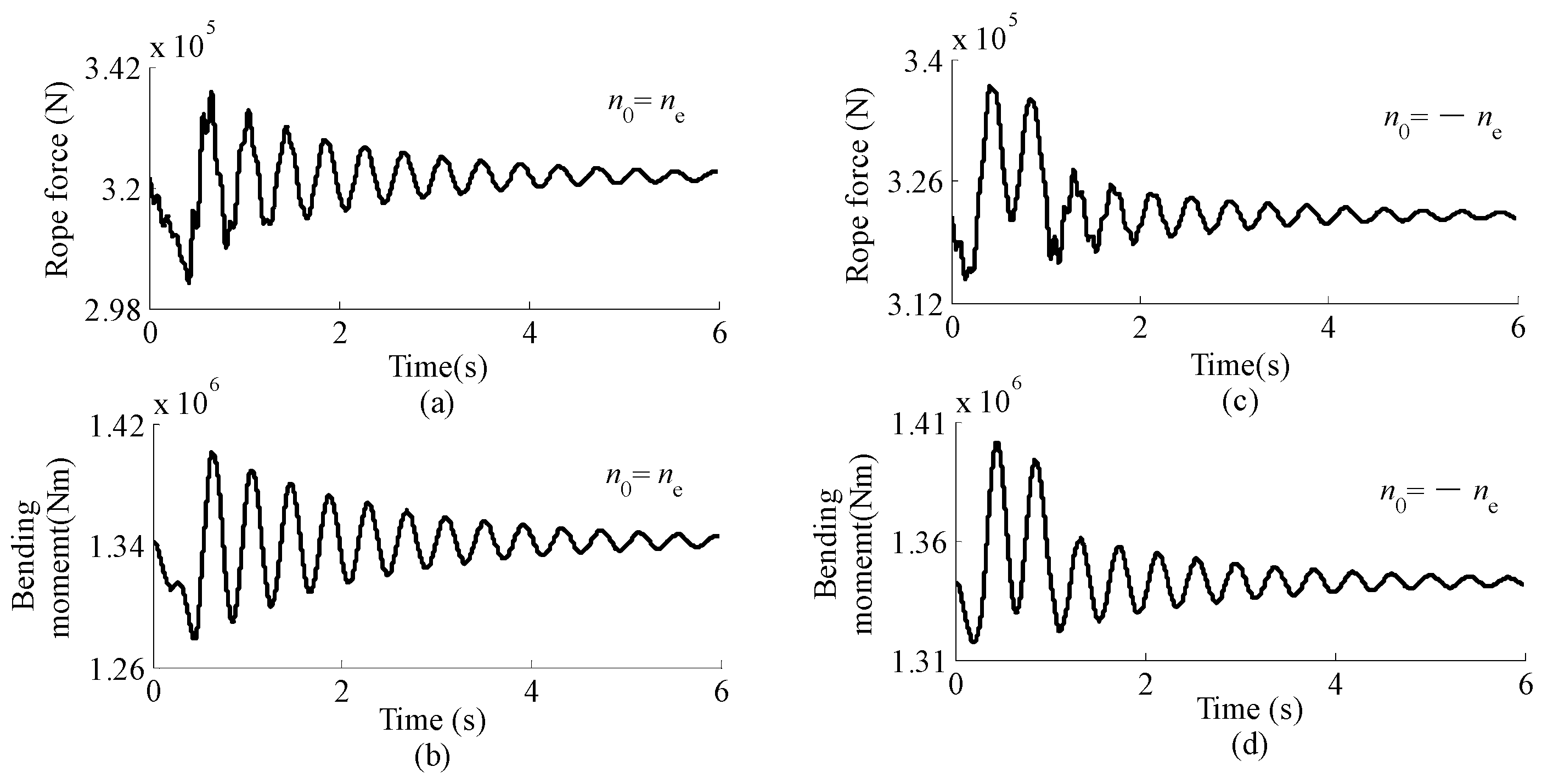
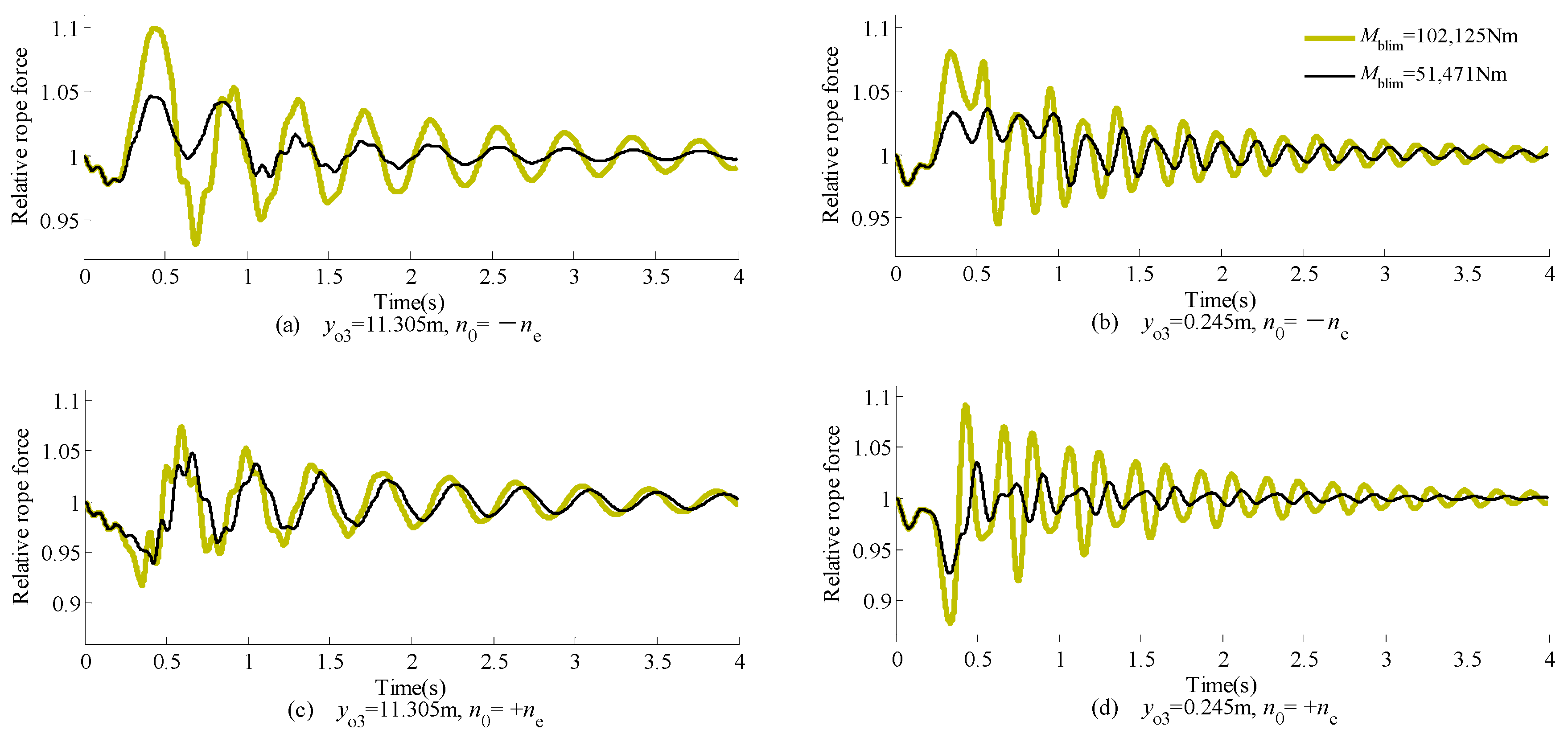
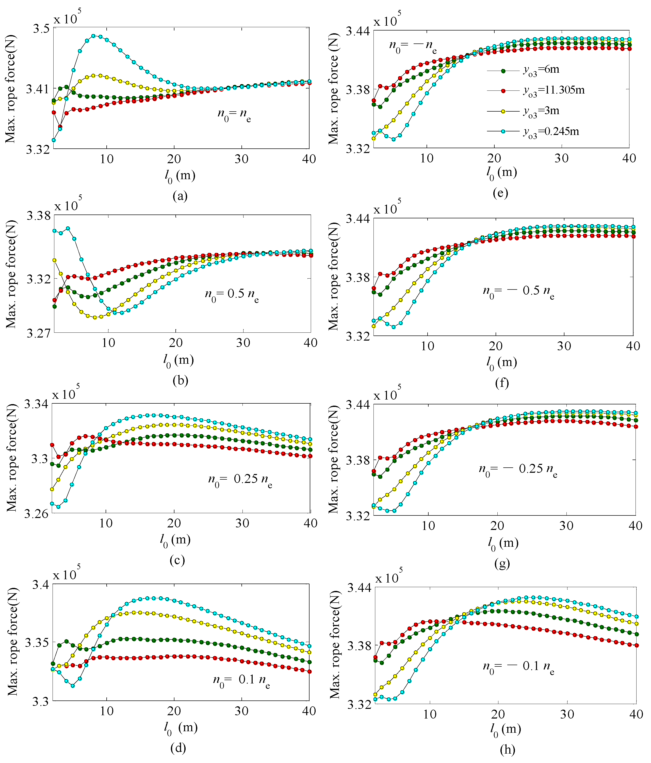
5.2. Time History of Rope Force and Bending Moment of Girder
6. Conclusions
- (1)
- The high-speed links in the lifting mechanism experience a fluctuating torque acting in two opposite directions with a non-zero mean during braking. This indicates that it is beneficial for increasing the working life of lifting mechanisms to avoid frequent emergency braking.
- (2)
- When a multi-brake scheme is adopted, the payload is unlikely to be supported equally by these brakes after completion of braking. The peak values of rope force and the bending moment of the girders may occur when braking a hoisting full-speed payload while the trolley is at the crane span end.
- (3)
- The magnitude of the payload, and the braking capacity and the action time of mechanical brakes are very important factors affecting the peak values and the range of internal forces acting on all components of the crane during braking. On the other hand, the position of the trolley mainly influences the internal forces acting on the steel rope and the girders.
- (4)
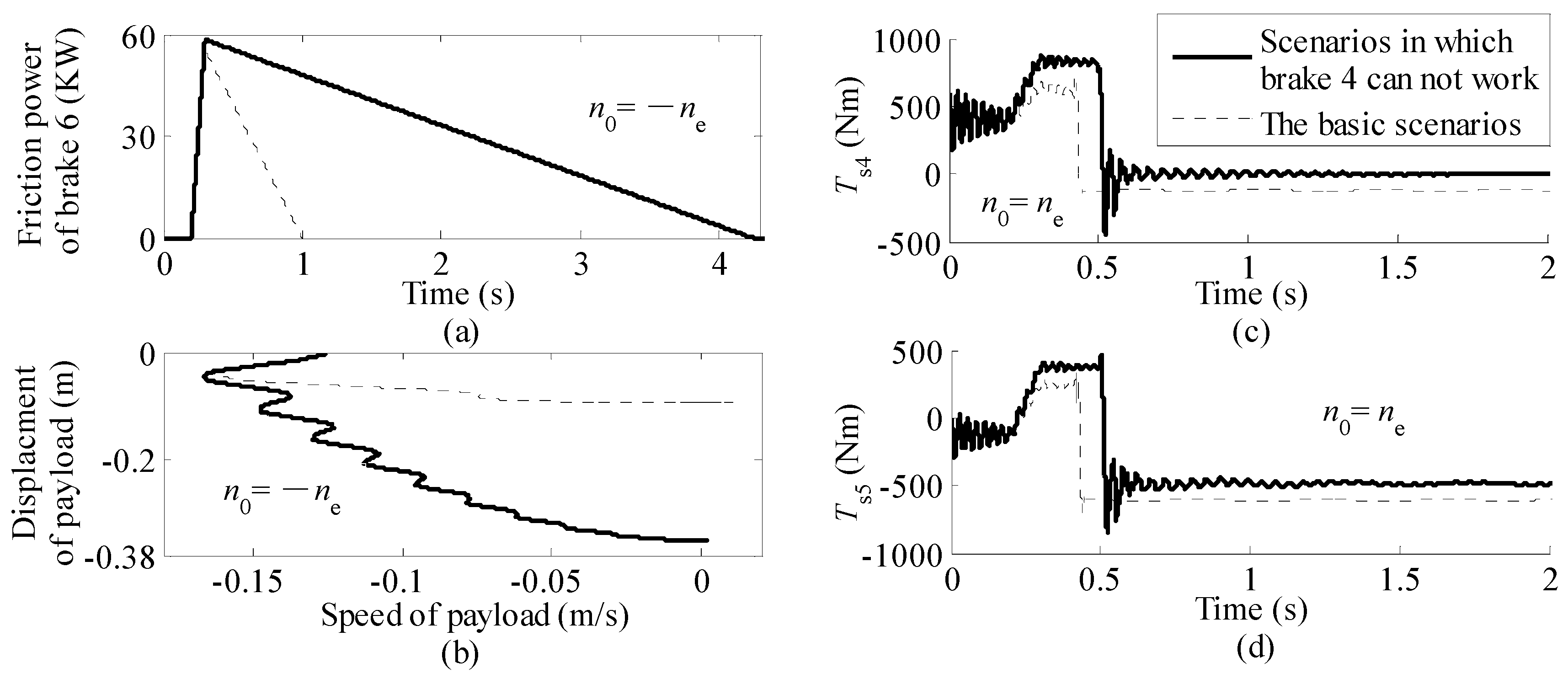
- The installation position of the mechanical brake and the action sequence when the multi-brake scheme is adopted may affect the loads acting on the high-speed links of the lifting mechanism. When the lifting mechanism with a dual-brake scheme is adopted, the load capacity of the high-speed links and the thermal capacity of friction pair of the brake are governed by the process when one of the two brakes ceases to work. In addition, the loads acting on components of cranes are higher if the braking capacity of the mechanical brakes is higher. Therefore, the two factors, i.e., the safety of cranes themselves and the capability of stopping and holding payloads safely, must be balanced when selecting the mechanical brakes.
- (5)
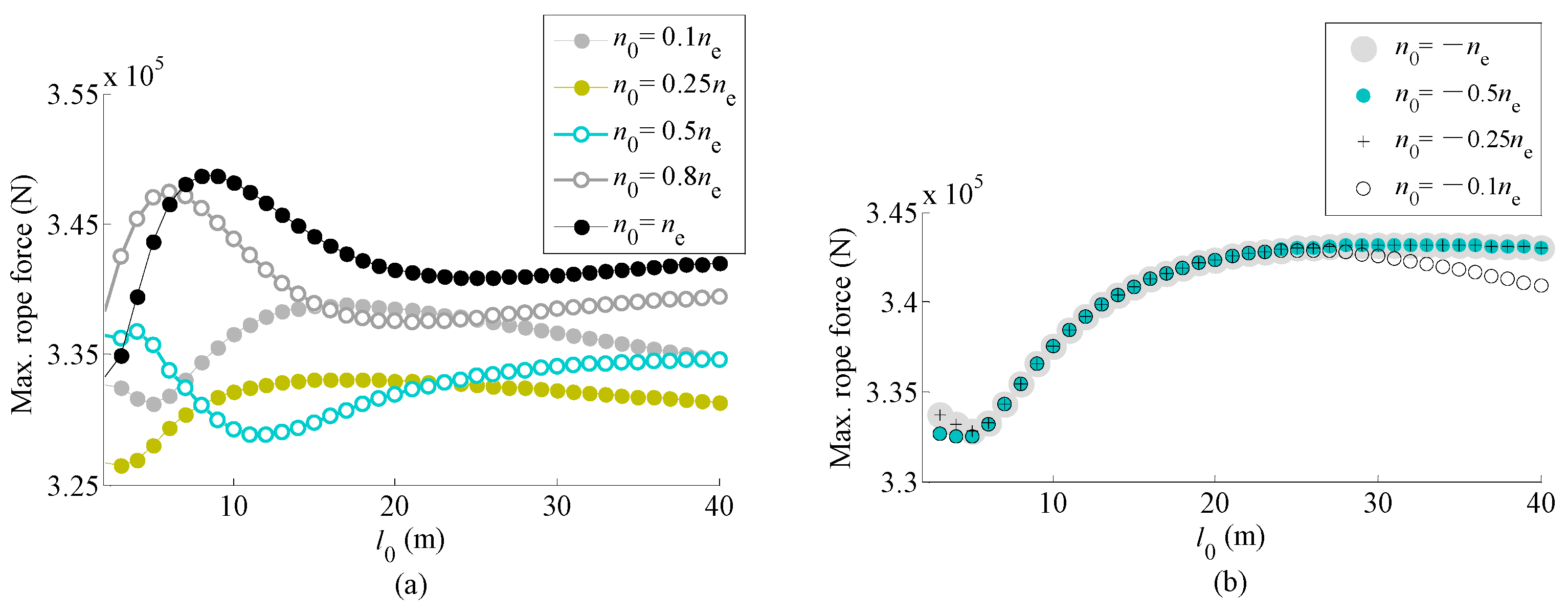
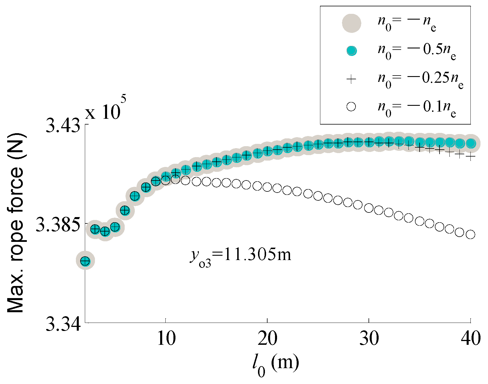
- The effect of the initial speed on the internal forces acting on the steel structure and the wire rope during braking of a hoisting payload is fairly different from that during braking of a lowering payload. Additionally, the peak values of the internal forces acting on the steel structure and the wire rope during braking process at a lower initial speed are not always smaller than those during braking at the full speed, i.e., as far as the steel structure and the wire rope of cranes are concerned, a braking process at a lower initial speed is not guaranteed to be safer than at full speed.
Author Contributions
Funding
Conflicts of Interest
Notation
| the vector of generalized coordinates used for describing elastic deformation of the girders along Z direction of the orthogonal coordinate system OXYZ | |
| b | the wheel base of the trolley |
| cg | the viscous damping coefficient of the material of the girder |
| cs | the viscous damping coefficient of transmission shafts in the lifting mechanism |
| cw | the viscous damping coefficient of the wire rope |
| kw | the total tensile force per unit strain of the wire rope segments hanging from the rope drum |
| ki | the torsional stiffness of the high-speed transmission shaft i in the lifting mechanism which is converted to a stiffness value in reference to the rope drum axis |
| l | the free length of the wire rope segments hanging from the rope drum |
| the free lengths of the rope hanging from the rope drum when the load-handling device is at its lower limit position | |
| the free lengths of the rope hanging from the rope drum when the basic braking scenario starts | |
| mg | the mass of a girder |
| ms | the reeving of the pulley block |
| the mass of the trolley | |
| mQ | the mass of the lifted object (including the load-handling device) |
| n | the number of generalized coordinates used for describing elastic deformation of the girders along Z direction of the orthogonal coordinate system OXYZ, |
| the rotating speed of driving motor in the lifting mechanism when braking starts | |
| the rated rotational speed of motor used for driving the lifting mechanism | |
| t0 | the starting instant of the integral interval of the equation of motion |
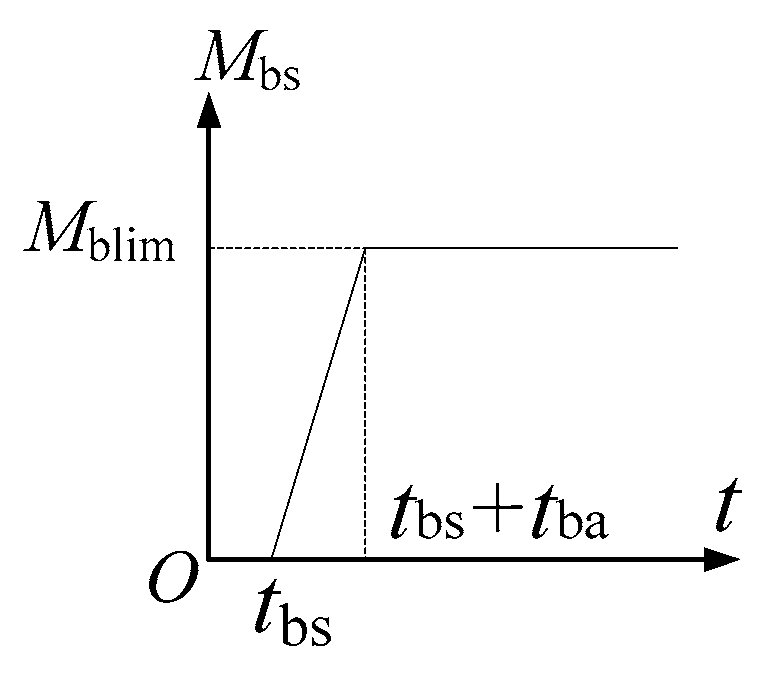
| the instant when the braking capacity of the brake starts to increase from zero | |
| the time interval when the braking capacity of the brake increases from zero to its maximum value | |
| tend | the ending instant of the integral interval of the equation of motion |
| the displacement of a point in the girder axis, whose Y coordinate in the orthogonal coordinate system OXYZ is y, relative to its position under the dead weight of the girder | |
| x0 | the initial value of the integration |
| the Y coordinate of the points on the trolley wheels axis | |
| the Y coordinate of the centres of wheels O3 and O3′ when wheels O4 and O4′ are located on the most unfavourable sections of the girders | |
| Ci | the constants involved in the elastic deformation due to the dead weight, the camber and the geometrical sizes of the girder, i=T, d |
| E | Young’s modulus of the girder material |
| Ix | the moment of inertia of the girder cross section with respect to its neutral axis, which is parallel to the X-axis of the orthogonal coordinate system OXYZ |
| the moment of inertia of the trolley with respect to its centroid axis, which is parallel to axis of the orthogonal coordinate system fixed to the trolley | |
| the moments of inertia of rotating rigid body i in the lifting mechanism which is converted to quantities in reference to the rope drum axis | |
| the modified Lagrangian function | |
| L | the span of the crane |
| the time function of the braking torque of the mechanical brake, which is converted to quantities in reference to the rope drum axis | |
| the maximum braking capacity of the brakes, which is converted to the corresponding quantity in reference to the axis of the rope drum | |
| the time function of the braking capacity of the brake i, which is converted to quantities in reference to the rope drum axis | |
| the resistance torque of the lifting mechanism | |
| Rd | the wrapping radius of the wire rope on the rope drum |
| T | the kinetic energy of the crane |
| the torque acting on the shaft used to connect components Ji and Ji+1 of the high-speed links in the lifting mechanism | |
| the potential energy of the crane | |
| the tensile strain of the wire rope segments hanging from the rope drum | |
| the efficiency of the lifting mechanism | |
| the angular displacement of rotating rigid body i in the lifting mechanism, which is converted to quantities in reference to the rope drum axis | |
| the Lagrange multiplier | |
| the friction coefficient between the rope drum groove and the wire rope | |
| the damping ratios corresponding to | |
| the damping ratios corresponding to | |
| the constraint which gives the relationship between l, and | |
| the coordinate of the points on the rope drum axis | |
| the coordinate of the gravity centre of the trolley |
References
- CEN. EN ISO13850 Safety of Machinery Emergency Stop Principles for Design; CEN: Brussels, Belgium, 2015. [Google Scholar]
- Olesiak, Z.; Pyryev, Y.; Yevtushenko, A. Determination of temperature and wear during braking. Wear 1997, 210, 120–126. [Google Scholar] [CrossRef]
- German Institute for Standardisation. DIN 15434-1-1989 Power Transmission Engineering—Principles for Drum- and Disc Brakes, Calculation; German Institute for Standardisation: Berlin, Germany, 1989. [Google Scholar]
- Severin, D.; Dörsch, S. Friction mechanism in industrial brakes. Wear 2001, 249, 771–779. [Google Scholar] [CrossRef]
- Wang, D.; Yin, J.; Zhu, Z.; Zhang, D.; Liu, D.; Liu, H.; Sun, F. Preparation of high friction brake shoe material and its tribological behaviors during emergency braking in ultra-deep coal mine hoist. Wear 2020, 458–459, 203391. [Google Scholar] [CrossRef]
- Wittenberghe, J.V.; Ost, W.; Baets, P.D. Testing the friction characteristics of industrial drum brake linings. Exp. Tech. 2012, 36, 43–49. [Google Scholar] [CrossRef]
- Park, K.P.; Cha, J.H.; Lee, K.Y. Dynamic factor analysis considering elastic boom effects in heavy lifting operations. Ocean Eng. 2011, 38, 1100–1113. [Google Scholar] [CrossRef]
- Sun, G.; Kleeberger, M.; Liu, J. Complete dynamic calculation of lattice mobile crane during hoisting motion. Mech. Mach. Theory 2005, 40, 447–466. [Google Scholar] [CrossRef]
- Posiadała, B. Influence of crane support system on motion of the lifted load. Mech. Mach. Theory 1997, 32, 9–20. [Google Scholar] [CrossRef]
- Ju, F.; Choo, Y.S.; Cui, F.S. Dynamic response of tower crane induced by the pendulum motion of the payload. Int. J. Solids Struct. 2006, 43, 376–389. [Google Scholar] [CrossRef] [Green Version]
- Jerman, B. An enhanced mathematical model for investigating the dynamic loading of a slewing crane. Proc. Inst. Mech. Eng. Part C J. Mech. Eng. Sci. 2006, 220, 421–433. [Google Scholar] [CrossRef]
- Cibicik, A.; Pedersen, E.; Egeland, O. Dynamics of luffing motion of a flexible knuckle boom crane actuated by hydraulic cylinders. Mech. Mach. Theory 2020, 143, 103616. [Google Scholar] [CrossRef]
- Yildirim, Ş.; Esim, E. A new approach for dynamic analysis of overhead crane systems under moving loads. In CONTROLO 2016, Proceedings of the 12th Portuguese Conference on Automatic Control, Guimarães, Portugal, 14–16 September 2016; Garrido, P., Soares, F., Moreira, A., Eds.; Springer: Cham, Switzerland, 2017; pp. 471–481. [Google Scholar]
- Urbaś, A. Computational implementation of the rigid finite element method in the statics and dynamics analysis of forest cranes. Appl. Math. Model. 2017, 46, 750–762. [Google Scholar] [CrossRef]
- Adamiec-Wójcik, I.; Drąg, Ł.; Metelski, M.; Nadratowski, K.; Wojciech, S. A 3D model for static and dynamic analysis of an offshore knuckle boom crane. Appl. Math. Model. 2019, 66, 256–274. [Google Scholar] [CrossRef]
- Cibicik, A.; Egeland, O. Dynamic modelling and force analysis of a knuckle boom crane using screw theory. Mech. Mach. Theory 2019, 133, 179–194. [Google Scholar] [CrossRef]
- Tomasz, H. Modeling the dynamics of cargo lifting process by overhead crane for dynamic overload factor estimation. J. Vibroeng. 2017, 19, 75–86. [Google Scholar]
- Zhao, Y.; Cheng, Z.; Sandvik, P.C.; Gao, Z.; Moan, T.; Van Buren, E. Numerical modeling and analysis of the dynamic motion response of an offshore wind turbine blade during installation by a jack-up crane vessel. Ocean Eng. 2018, 165, 353–364. [Google Scholar] [CrossRef]
- Cekus, D.; Gnatowska, R.; Kwiatoń, P. Impact of wind on the movement of the load carried by rotary crane. Appl. Sci. 2019, 9, 3842. [Google Scholar] [CrossRef] [Green Version]
- Ramli, L.; Mohamed, Z.; Abdullahi, A.M.; Jaafar, H.I.; Lazim, I.M. Control strategies for crane systems: A comprehensive review. Mech. Syst. Signal Process. 2017, 95, 1–23. [Google Scholar] [CrossRef]
- Tomczyk, J.; Cink, J.; Kosucki, A. Dynamics of an overhead crane under a wind disturbance condition. Autom. Constr. 2014, 42, 100–111. [Google Scholar] [CrossRef]
- Abdullahi, A.M.; Mohamed, Z.; Selamat, H.; Pota, H.R.; Zainal Abidin, M.S.; Fasih, S.M. Efficient control of a 3D overhead crane with simultaneous payload hoisting and wind disturbance: Design, simulation and experiment. Mech. Syst. Signal Process. 2020, 145, 106893. [Google Scholar] [CrossRef]
- Zhao, X.; Huang, J. Distributed-mass payload dynamics and control of dual cranes undergoing planar motions. Mech. Syst. Signal Process. 2019, 126, 636–648. [Google Scholar] [CrossRef]
- Wu, Q.; Wang, X.; Hua, L.; Xia, M. Dynamic analysis and time optimal anti-swing control of double pendulum bridge crane with distributed mass beams. Mech. Syst. Signal Process. 2020, 144, 106968. [Google Scholar] [CrossRef]
- Zhang, M.; Zhang, Y.; Ji, B.; Ma, C.; Cheng, X. Adaptive sway reduction for tower crane systems with varying cable lengths. Autom. Constr. 2020, 119, 103342. [Google Scholar] [CrossRef]
- Otani, A.; Nagashima, K.; Suzuki, J. Vertical seismic response of overhead crane. Nucl. Eng. Des. 2002, 212, 211–220. [Google Scholar] [CrossRef] [Green Version]
- Kobayashi, N.; Kuribara, H.; Honda, T.; Watanabe, M. Nonlinear seismic responses of container cranes including the contact problem between wheels and rails. J. Press. Vessel Technol. 2004, 126, 59–65. [Google Scholar] [CrossRef]
- Feau, C.; Politopoulos, I.; Kamaris, G.; Mathey, C.; Chaudat, T.; Nahas, G. Experimental and numerical investigation of the earthquake response of crane bridges. Eng. Struct. 2015, 84, 89–101. [Google Scholar] [CrossRef]
- Huh, J.; Nguyen, V.B.; Tran, Q.H.; Ahn, J.-H.; Kang, C. Effects of boundary condition models on the seismic responses of a container crane. Appl. Sci. 2019, 9, 241. [Google Scholar] [CrossRef] [Green Version]
- Chen, H.; Xuan, B.; Yang, P.; Chen, H. A new overhead crane emergency braking method with theoretical analysis and experimental verification. Nonlinear Dyn. 2019, 98, 2211–2225. [Google Scholar] [CrossRef]
- Vöth, S. Emergency braking of fast running coal handling gantry hoists. In Proceedings of the XVII International Coal Preparation Congress, Saint-Petersburg, Russia, 28 June–1 July 2016; Litvinenko, V., Ed.; Springer: Cham, Switzerland, 2016; pp. 135–140. [Google Scholar]
- Streltsov, S.V.; Ryzhikov, V.A. Influence of uneven braking of running wheels on stress-strain state of crane metal structure. In Lecture Notes in Mechanical Engineering, Proceedings of the 4th International Conference on Industrial Engineering, Moscow, Russia, 15–18 May 2018; Radionov, A., Kravchenko, O., Eds.; Springer: Cham, Switzerland, 2018; pp. 2055–2062. [Google Scholar]
- Singer, N.C.; Seering, W.P. Preshaping command inputs to reduce system vibration. J. Dyn. Syst. Meas. Control 1990, 112, 76–82. [Google Scholar] [CrossRef]
- Singhose, W. Command shaping for flexible systems: A review of the first 50 years. Int. J. Precis. Eng. Manuf. 2009, 10, 153–168. [Google Scholar] [CrossRef]
- Manning, R.; Clement, J.; Kim, D.; Singhose, W.E. Dynamics and control of bridge cranes transporting distributed-mass payloads. J. Dyn. Syst. Meas. Control 2010, 132, 014505. [Google Scholar] [CrossRef]
- BSI. BS EN 13001-2-2004+A3-2009 Crane Safety-General Design Part 2: Load Actions; BSI: London, UK, 2009. [Google Scholar]
- BSI. BS EN 13001-1-2004+A1-2009 Crane Safety-General Design Part 1: General Principles and Requirements; BSI: London, UK, 2009. [Google Scholar]
- Niu, C.M.; Zhang, H.W.; Ouyang, H. A comprehensive dynamic model of electric overhead cranes and the lifting operations. Proc. Inst. Mech. Eng. Part C J. Mech. Eng. Sci. 2012, 226, 1484–1503. [Google Scholar] [CrossRef]
- Feyrer, K. Wire Ropes-Tension, Endurance, Reliability, 2nd ed.; Springer: Berlin/Heidelberg, Germany, 2015. [Google Scholar]


Publisher’s Note: MDPI stays neutral with regard to jurisdictional claims in published maps and institutional affiliations. |
© 2020 by the authors. Licensee MDPI, Basel, Switzerland. This article is an open access article distributed under the terms and conditions of the Creative Commons Attribution (CC BY) license (http://creativecommons.org/licenses/by/4.0/).
Share and Cite
Niu, C.; Ouyang, H. Nonlinear Dynamic Analysis of Lifting Mechanism of an Electric Overhead Crane during Emergency Braking. Appl. Sci. 2020, 10, 8334. https://doi.org/10.3390/app10238334
Niu C, Ouyang H. Nonlinear Dynamic Analysis of Lifting Mechanism of an Electric Overhead Crane during Emergency Braking. Applied Sciences. 2020; 10(23):8334. https://doi.org/10.3390/app10238334
Chicago/Turabian StyleNiu, Congmin, and Huajiang Ouyang. 2020. "Nonlinear Dynamic Analysis of Lifting Mechanism of an Electric Overhead Crane during Emergency Braking" Applied Sciences 10, no. 23: 8334. https://doi.org/10.3390/app10238334