Abstract
Metabolic Syndrome (MetS) is a set of risk factors that increase the probability of heart disease or even diabetes mellitus. The diagnosis of the pathology implies compliance with at least three of five risk factors. Doctors obtain two of those factors in a medical consultation: waist circumference and blood pressure. The other three factors are biochemical variables that require a blood test to determine triglyceride, high-density lipoprotein cholesterol, and fasting plasma glucose. Consequently, scientists are developing technology for non-invasive diagnostics, but medical personnel also need the risk factors involved in MetS to start a treatment. This paper describes the segmentation of MetS into ten types based on harmonized Metabolic Syndrome criteria. It proposes a framework to diagnose the types of MetS based on Artificial Neural Networks and Random undersampling Boosted tree using non-biochemical variables such as anthropometric and clinical information. The framework works over imbalanced and balanced datasets using the Synthetic Minority Oversampling Technique and for validation uses random subsampling to get performance evaluation indicators between the classifiers. The results showed an excellent framework for diagnosing the 10 MetS types that have Area under Receiver Operating Characteristic (AROC) curves with a range of 71% to 93% compared with AROC 82.86% from traditional MetS.
1. Introduction
Metabolic syndrome (MetS) is not a worldwide recognized cause of death. However, it is a trigger that increases the chances of multi-systemically and progressively affecting the people who suffer from it, and that creates a pattern of metabolic abnormalities that reflect in the factors associated with the increase in mortality due to diabetes mellitus or Coronary Heart Disease (CHD) [1,2]. These are non-communicable diseases and are the leading causes of mortality worldwide [3,4]. Patients who have four out of five significant variables have a 3.7 times higher risk of experiencing cardiac events and 24.5 times more risk of being diagnosed with type 2 diabetes [5].
MetS is coded E88.81 according to the International Classification of Diseases, 10th Edition (ICD- 10, 2020 version) and is a group of alterations in metabolism that includes dyslipidemia (abnormal concentrations of lipids in the blood: increased triglycerides and decreased HDL cholesterol), hypertension, hyperglycemia, and obesity [6]. The insidious increase in the elements of MetS, obesity, insulin resistance (IR), and dyslipidemia are responsible for the current global epidemic of type 2 diabetes [5]. Other authors relate MetS with the occurrence of cancers and chronic kidney disease [7,8].
The available evidence indicates that in most countries, between 20% and 30% of the adult population can be characterized as having MetS. In some populations or segments of the population, the MetS prevalence is even higher [9,10]. The prevalence of the syndrome in countries such as the United States has increased. Three studies have yielded the following results: 23.7% in 2002, 34.2% in 2006 [11,12] and nearly 34.7% of all U.S. adults were estimated to have the MetS in 2011–2012. During the period 2003–2012, the MetS prevalence was estimated at 50% in adults older than 60 years of age [13].
The Kuopio Ischaemic Heart Disease, Risk Factor Study consisted of a population-based, prospective cohort study of 1209 Finnish men aged 42 to 60 years at baseline (1984–1989), who did not initially present cardiovascular disease, cancer, or diabetes. They found that men with the Metabolic Syndrome as defined by the National Cholesterol Education Programme Adult Treatment Panel III (NCEP ATP III) were 2.9 (95% confidence interval [CI], 1.2–7.2) to 4.2 (95% CI, 1.6–10.8) times more likely to die of CHD [14]. Moreover, a review study showed a range of Odds Ratio (OR) three- and 20-fold for developing type 2 diabetes. Thus, it is often considered prediabetes [15,16].
MetS prevalence in some Latin American countries is high. For example, Mexico has more than 40% prevalence in adults [17]. In Colombia, several studies about the prevalence of the syndrome have focused on specific population ranges. For instance, a short study of 62 people in a northern city of Colombia found that the patients with arterial hypertension showed a very high prevalence level (74.2%) of Metabolic Syndrome, according to the ATP III criteria [5,18].
Healthcare professionals diagnose the syndrome with a set of risk factors using some threshold levels in the criteria proposed by several medical associations. Several associations have proposed criteria, including the World Health Organization (WHO) [19], the Adult Treatment Panel of the National Cholesterol Education Program (ATP III) [20], the European Group for the study of Insulin Resistance (EGIR) [21], and the International Diabetes Federation (IDF) [22]. Since 2009, specialists arrived at the consensus of a Harmonized Metabolic Syndrome (HMS) through a joint interim statement that several associations and institutes write to unify the diagnosis criteria [23].
Most of the criteria for diagnosing MetS agree that patients must have at least three of the five risk factors to be diagnosed. The contrast is IDF, which requires central obesity plus two more taken from the remaining four risk factors. For the population of Colombia, according to the HMS criterion, which is the most updated, the waist circumference levels in men must be ≥90 cm and in females must be ≥80 cm to have central obesity. The other risk factors are shown in Table 1.

Table 1.
Definition of the MetS according to HMS (Data from [16]).
Independently of the criteria to diagnose MetS, the diagnosis uses five factors. Doctors get two of those factors (Waist Circumference (WC) and Blood Pressure (BP)) in medical consultations and a community setting. Invasive tests are required to know the value of triglycerides, HDL-C, and fasting plasma glucose present in the patient’s blood. Therefore, the time of treatment initiation can vary according to the health system. The delay between initial consultation, a blood test to measure the triglycerides, fasting blood sugar, and HDL-C levels, plus a diagnostic consultation, can add several days or weeks [24,25] creating a problem to diagnose early.
This time delay in obtaining the results, particularly for patients in remote locations, might be sufficient time in some cases to worsen or aggravate the patient’s health conditions due to the occurrence of a stroke diabetes [26]. It is useful to diagnose early MetS to avoid or delay the onset of some illnesses already mentioned.
Many researchers have proposed solving the problem without doing a blood test using machine learning techniques, such as Kroon et al. [27], Hsiung et al. [28] and others. However, when diagnosing MetS, doctors always check the triglycerides, fasting plasma glucose, and HDL-C values to recommend a specific treatment to prevent diabetes or coronary diseases. They also want to know the possible cause since it allows a better decision to plan patient treatment [23,29].
Therefore, this article proposes segmenting MetS into various types to identify the risk factors that produce it and use machine learning to diagnose them early without making a blood test and comparing each MetS type with the traditional MetS. We used four approaches for improving the accuracy or AROC for the different MetS types. The first approach uses the ANN technique; the second approach uses an ensemble classification algorithm as the Random undersampling Boosted tree (RusBoost) ensemble. The third approach uses an oversampling technique to create more data and then applying ANN. The last approach uses the dataset with oversampling and RusBoost.
The objectives of this paper are the following:
- Achieve a mathematical representation to diagnose MetS using HMS criteria.
- Propose a segmentation of MetS using HMS criteria.
- Develop a framework to diagnose the different MetS types according to HMS criteria using a set of variables that doctors can obtain using non-invasive methods in a first consultation.
- Evaluate two machine learning techniques using performance indicators for each MetS type.
We now continue to explain the methodology to design a framework to diagnose each MetS type without doing a blood test based on MetS segmentation. Then, we show the results of the implementation and then the discussion and conclusion.
2. Methodology
This paper uses a novel methodology called RAMAD to develop the article. This RAMAD methodology [30] has five stages and improves the model every time by cycling until it achieves the design of a generalized model based on their data, as described in Figure 1.
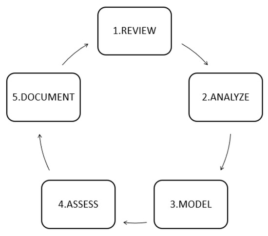
Figure 1.
RAMAD methodology [30].
The execution of the steps can be updated. Researchers could do so by repeating the methodology from the first phase. In this way, they could add new models from the literature. This circular approach ensures that researchers keep improving their models. If they follow the documentation phase correctly, new researchers could improve the original model’s prediction capabilities.
2.1. Review
The Review phase performed a specialized search in the following databases: DBLP, IEEE, and ACM for the relationship with Computer Science, and Pubmed for its relationship with healthcare research. We have used a window of 12 years since 2008. The keywords used are “SEGMENTATION” OR “TYPES” OR “PREDICTION” OR “ANN” AND [“METABOLIC SYNDROME” AND “WITHOUT BLOOD TEST”] for Query1: IEEE, Query2: DBLP, Query3: ACM, and Query4: PUBMED to know all the projects related to keywords in these search engines dedicated to the field of engineering. The results of the queries (QUERY1: 92, QUERY2: 51, QUERY3: 82, and QUERY4: 131) provided an extensive list of journal articles and conferences. However, not all the documents are directly related to the segmentation of MetS since DBLP, IEEE XPLORE, ACM, and PUBMED delivered articles on machine learning and computer science at a general level, for example, the topic image segmentation.
Then, the delivered list was filtered, evaluating its relationship with the segmentation of MetS or types of MetS. It excluded repeated articles (mirror articles). Afterward, we performed a manual inspection and then filtered by the criteria established on the following questions.
- Could authors predict the Metabolic Syndrome types or segmentation without a blood test? Y/N.
- What Metabolic Syndrome diagnostic criteria did the authors use? e.g., ATP II, IDF, HMS, or other criteria recognized.
- What ANN configuration did the authors use?
- What validation method did the authors use? e.g., hold out, random subsampling, and others.
- What performance indicators did the authors use? e.g., Sensitivity, Area Under the ROC curve, Specificity.
The manual inspection did not find anything about the segmentation of MetS using only variables obtained in a medical consultation such as anthropometric and clinical or history variables. However, we found three articles that diagnose MetS using ANN and anthropometric and clinical variables such as Age, Sex, Weight, Height, Waist Circumference (WC), Hip Circumference (HC), Waist to Hip ratio (WHHR), Waist to Stature (WSR), Body Mass Index (BMI), Body Fat Percentage (BFP), Systole Blood Pressure (SBP) and Diastole Blood Pressure (DBP). These variables will be used to build the model to diagnose the MetS types without doing a blood test, i.e., without using biochemical variables.
As a summary, Table 2 shows an overview of the variables that are used explicitly in the study and other variables that were not used (implicitly) but are necessary to construct the explicit variables. It also shows the classification models used for the MetS diagnosis without taking a blood sample of each article in the literature, and we describe them now:
Table 2.
Variables and hidden neurons of ANN used by the authors found in the review.
Murguia-Romero et al. [31] configured an Artificial Neural Network (ANN) based on Multilayer Perceptron (MLP) with back-propagation of 25 hidden neurons to diagnose with HMS criteria and using BMI, WC, Weight, Height, and Sex variables from a dataset with 826 people to validate using 70% for training and 30% for testing.
Chen et al. [32] used anthropometric and clinical variables such as HC, Age, BMI, WC, WHR, Sex, SBP, and DBP, and implicitly used Weight and Height as inputs of a back-propagation neural network (BPNN). They diagnosed the MetS and compared the results with another machine learning technique, Principal Component Logistic Regression (PCLR), for predicting Met with IDF criteria using a dataset of 2074 individuals (male: 1495, female: 579), obtaining improved results in the BPNN.
Kupusinac et al. [33] presented a feed-forward ANN with back-propagation for diagnosing the MetS with IDF criteria using non-invasive variables such as sex, age, BMI, WHR, SBP, DBP, and in an implicit way WC, Weight, Height, due to the use of WSR and BMI. The dataset of 2928 people was divided into three parts with the proportion 80:10:10 for the stage of training, validation, and testing.
Diagnosing MetS using non-biochemical variables is an approach that implies not taking blood samples. This approach can help doctors make early decisions about MetS. However, doctors always need to know what risk factors are present in the patient diagnosed with MetS to start treatment early to decrease the probability of heart disease or diabetes mellitus type 2. Moreover, to date, no study has evaluated the MetS types or the segmentation of MetS from a perspective of machine learning. This situation may be due to the lack of a model of segmentation of MetS that explains the different MetS types.
2.2. Analysis
2.2.1. Design and Study Population
Universidad del Norte obtained the data through a study performed in the second semester of 2012, as an integrated research strategy for the study and intervention of the Metabolic Syndrome in Barranquilla, Colombia, using the following rules:
List of inclusion rules
- Age of 20 years or over.
- The subject can understand the instructions explained by the researchers.
- The subject can sign an informed consent.
- The subject resides permanently in the area.
List of exclusion rules
- Are you pregnant?
- Are you bedridden?
The study began with a survey of 615 adult subjects 20 years old or older randomly selected in 10 city neighborhoods and distributed proportionally according to the neighborhood, and residence block. The survey consisted of several questions divided into several sections. The most relevant sections are obesity history, anthropometric measurements, and biochemical blood measurements such as lipid profile (cholesterol, triglycerides), fasting plasma glucose. The study determined Metabolic Syndrome and associated factors using the laboratory results plus the surveys’ data and the weight measurements, size, and abdominal perimeter.
As a limitation of the study, the researchers initially designed it to diagnose the traditional MetS, not to diagnose different MetS types because there was no hypothesis about MetS segmentation at that date. However, we consider that the patients’ predictive variables are reliable to diagnose the traditional MetS, and in the same way, it will be reliable to diagnose the different MetS types.
The research was carried out under the Good Clinical Practices (GCP) guide and the International Conference on Harmonization (ICH). Therefore, respect for the dignity and the protection of the rights and well-being of people prevailed. The study included protecting the individuals’ privacy and autonomy and the decision not to participate in the survey. It is important to note that there was no risk of the participant suffering any damage due to the study. The data that support the findings of this study are available from the corresponding author, upon reasonable request.
This research ensures compliance with the guidelines for the protection of research subjects. Participants received a letter informing them about the project and their rights as participants. The research was approved by the Ethics Committee of the Universidad del Norte in act 87 in September 2012 and complies with the national guidelines (Resolution No. 8430 of the Ministry of Health of Colombia) and international guidelines (the Declaration of Helsinki) related to the participants’ informed consent.
2.2.2. Physical Examination and Blood Tests
The respondents arrived at the University del Norte’s hospital, where healthcare professionals performed the scheduled clinical examination, executed by a Doctor and a nurse. They measured Blood pressure and took two doses with an interval of 5 min, averaging the two measurements. Nurses measured stature and weight, without shoes and with the least amount of clothes possible. They also measured waist and hip circumferences.
Many articles have supported the association between MetS and the percentage of body fat obtained with the bioimpedance technique [34,35]. However, according to the objectives stated above, the variables should be obtained from the medical consultation data where in general, the first level assistance office does not have a body fat measurement device.
Therefore, the measurement of Body Fat Percentage (BFP) was performed with the following equations depending on gender for men Equation (1) and for women Equation (2). According to an analysis of the authors Lean, Han, and Deurenberg [36], Equations (1) and (2) have the largest prediction power to measure BFP.
The research also obtained information about the respondents’ health history that was recommended by several authors [27,28,32]. According to the variables we have in the study, we only analyze the history of obesity with the variable obtained from the following question: “Have any health professionals diagnosed you with overweight or obesity?”. Recent studies have shown a strong association of the previous obesity diagnosis to the risk of heart failure (HF) [37]. Therefore, we tabulate the discrete values of the Previous Obesity Diagnosis (POD) variable in the Results section.
2.3. Model
In this section, we explain the mathematical representation to diagnose the MetS using HMS. Moreover, we propose a model of segmentation of MetS obtaining several types of MetS for HMS criteria. Then, we show an abstract overview of a framework for implementing the proposed method to predict each type of MetS without doing a blood test.
2.3.1. Mathematical Representation to Diagnose MetS
The MetS, according to different traditional organizations (HMS, IDF, ATP III, among others), must be diagnosed when the patient meets at least three risk factors. We base the verification of a risk factor through the criteria shown in Table 1. Then we could represent each risk factor as a dichotomous variable, where 1 is positive and 0 is negative. Therefore, the diagnosis with the HMS criterion can be represented mathematically through the sum of dichotomous variables greater than or equal to three positive risk factors, as shown in Equation (3).
- W: Represents the normal(0) or raised(1) status of the dichotomous values of the waist circumference
- P: Represents the normal(0) or raised(1) status of the dichotomous variable of the blood pressure
- G: Represents the normal(0) or raised(1) status of the dichotomous variable of the fasting plasma glucose
- H: Represents the normal(0) or lower(1) status of the dichotomous variable of the HDL-C
- T: Represents the normal(0) or raised(1) status of the dichotomous variable of the triglycerides
Equation (3) shows the interaction of the dichotomous variables of triglycerides, fasting plasma glucose, HDL-C, waist circumference, and blood pressure used to diagnose the MetS.
It is essential to keep in mind that we obtain the dichotomous variable of blood pressure (P) by making a logical OR operation between the dichotomous variables of Systolic Blood Pressure () and Diastolic Blood Pressure (), as shown in Equation (4).
2.3.2. Proposed Model MetS Segmentation
Several researchers have shown that it is possible to diagnose MetS using only non-biochemical variables [27,28,30]. However, doctors also require information about the variables that cause the syndrome to proceed with the appropriate treatment to prevent diabetes or coronary diseases. Therefore, there are several cases of MetS due to the combination of the five(5) [23,29] dichotomous values of risk factors represented by , which are in base 2. With five factors, there are = 32 combinations (00000 to 11111) and each combination represents a case of MetS that doctors diagnose as positive or negative based on the HMS criteria. To determine each positive case of MetS, we built a true table of all MetS cases using HMS criteria with a Boolean perspective [38,39] as shown in Table 3. The first column with the n values represents in base 10, all the combinations of the dichotomous values of risk factors , which are in base 2. The MetS column represents the syndrome diagnosis. The value is positive (1) if three or more dichotomous values are positive. Otherwise, the column is negative (0). For example, in the case when , the combination in base 2 represents 10011, which converted to base 10 is 19. We also can use an apostrophe as a negation of a value. The same example then can also be represented as .
Table 3.
Truth table of all the combinations of the risk factors of the MetS according to the HMS criteria.
We find the different cases of MetS according to Table 3 and to HMS criterion giving a result of a sum of products of the dichotomous values of the risk factors represented numerically in base 10, as shown in Equation (5).
For the traditional MetS, we also call it general MetS to separate it from the MetS types proposed in this article. Next, we optimize Equation (5) and minimize it using the Quine–McCluskey algorithm. The detailed solution is in Appendix A and we checked the technique with Karnaugh Map as well, obtaining Equation (6) in the format .
As observed in Equation (6), the tripartite variables that we call MetS types are always necessary for a diagnosis of the traditional MetS. It requires at least one of these , , , , , , , , , and to be positive according to the HMS criteria, as detailed in Table 4.
Table 4.
Types of MetS according to the HMS criterion.
We will use the term traditional MetS or general MetS to separate it from the MetS types proposed in this article. For practical purposes, we developed a framework to diagnose the MetS types based on Equation (6) representing the HMS criteria using machine learning techniques.
2.3.3. Framework to Diagnose the MetS Types
Figure 2 shows an abstract overview of the implementation of the proposed method by using a framework divided into three stages.
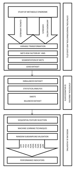
Figure 2.
Framework to diagnose the types of MetS by HMS criterion using non-biochemical variables.
- (a)
- Extraction, Transformation, and Load (ETL)In this stage, we collected the data from a population of 615 subjects who authorized taking a blood sample to measure the values of triglycerides, HDL-C, and fasting plasma glucose. Moreover, the study recorded the anthropometric and clinical variables such as Age, Sex, Weight, Height, Waist Circumference (WC), Hip Circumference (HC), Systole Blood Pressure (SBP), and Diastole Blood Pressure (DBP).Later, through the transformation process, we obtained Body Mass Index, Body Fat Percentage, Waist Hip circumference ratio, Dichotomous Blood Pressure Systolic, Dichotomous Diastolic Blood Pressure, Dichotomous Blood Pressure, Dichotomous triglycerides, Dichotomous fasting blood sugar, Dichotomous HDL-C, and Dichotomous Waist circumference among others.Afterward, we used dichotomous values of the HMS criteria’ risk factors to build the different MetS types obtained from the segmentation process explained in the previous subsection. We obtained the output variables WPG, WPH, WPT, WGH, WGT, WTH, PGT, PGH, PHT, and GHT. Therefore, all anthropometric and clinical data was loaded in a dataset of 615 records.
- (b)
- Statistical analysis and balancing datasetIn this stage, we began with a dataset containing 615 people with samples of biochemical variables with their respective diagnostic of MetS. Then, we did a descriptive statistical analysis of the dataset, finding that some types of MetS were imbalanced, as shown in the Results section.This problem was caused by the low prevalence of the risk factor for fasting blood glucose in the study population. This low prevalence is expected in a study of MetS [40]. We resolved this imbalance by using a data balancing technique, such as the Synthetic Minority Oversampling Technique (SMOTE) [41,42] implemented by WEKA. We created synthetic data to get a balanced dataset of 799 records (615 plus 184 synthetic data) and a better distribution of risk factors of MetS, thus improving the quality of discrimination.
- (c)
- ModelingIn this stage, we use an algorithm to select the necessary non-biochemical features. We used Sequential Feature Selection in Matlab to achieve the maximum discrimination in both datasets (imbalanced and balanced) of the proposed model’s output variables.For the following step, we used several Multilayer Perceptron (MLP) ANN to predict each MetS type: WPG, WPH, WPT, WGH, WGT, WTH, PGT, PGH, PTH, and GHT. These ANN should be trained before being used to predict the output variable value, i.e., the dependent variable. Each ANN is formed by neurons whose elements are a set of inputs that can come from other neurons or the outside, as shown in Figure 3 the basic structure of an ANN.
 Figure 3. Basic structure of the artificial neural network.Each structure of ANN should be initialized according to the propagation rule to the starting and each node has synaptic weights, which are the degree of communication between neurons, as shown Equations (7) and (8). Then, the data used to train the network is introduced into the network after the propagation algorithm is employed to obtain the final parameters in the network. In practice, the algorithm is divided into two parts: network training and network testing. The steps of propagation algorithm are described as follows [43]:where are inputs, are synaptic weights, are bias in the input layer, k is the iteration and n is the number of inputs resulting in a net output that is determined by a activation function with output [44,45].This information flows in one direction only from the inputs to the hidden layer and after to the output layer, i.e., the information that comes from different activation function neurons, which is responsible for determining the current state and finally converges all the data to the output [33].Each ANN has several hidden neurons that have functions, such as the hyperbolic tangent sigmoid function and an output layer with a neuron. The neuron has a function that can be a log-sigmoid function [44,46].It should be noted that there are no hard and fast rules for the number of hidden neurons. These hidden neurons can be calculated or found empirically and are highly dependent on the problem and the dataset [47]. However, we used the methodology mentioned by [48,49,50] and described in Equation (9), where the number of hidden neurons (NHN) can be of the input variables plus an output variable.We used Equation (9), to estimate the number of hidden neurons to contribute to research in the area of machine learning for the diagnosis of MetS without using biochemical variables and in a way, describe every detail of the process for experimentation by other researchers can continue investigating these models as well as Chen [32] that used other equation to calculate the hidden neurons.Another machine learning technique used to diagnose the MetS types was the ensemble Random undersampling Boosted tree (RusBoost) because the data from the MetS study is imbalanced [51]. This technique improves the performance indicators of models using imbalanced data by applying a random undersampling technique. The technique randomly removes samples from the majority class [52], as shown in the algorithm detailed in Appendix B with the configuration showed in Table 5.
Table 5. RusBoost Configuration.
Figure 3. Basic structure of the artificial neural network.Each structure of ANN should be initialized according to the propagation rule to the starting and each node has synaptic weights, which are the degree of communication between neurons, as shown Equations (7) and (8). Then, the data used to train the network is introduced into the network after the propagation algorithm is employed to obtain the final parameters in the network. In practice, the algorithm is divided into two parts: network training and network testing. The steps of propagation algorithm are described as follows [43]:where are inputs, are synaptic weights, are bias in the input layer, k is the iteration and n is the number of inputs resulting in a net output that is determined by a activation function with output [44,45].This information flows in one direction only from the inputs to the hidden layer and after to the output layer, i.e., the information that comes from different activation function neurons, which is responsible for determining the current state and finally converges all the data to the output [33].Each ANN has several hidden neurons that have functions, such as the hyperbolic tangent sigmoid function and an output layer with a neuron. The neuron has a function that can be a log-sigmoid function [44,46].It should be noted that there are no hard and fast rules for the number of hidden neurons. These hidden neurons can be calculated or found empirically and are highly dependent on the problem and the dataset [47]. However, we used the methodology mentioned by [48,49,50] and described in Equation (9), where the number of hidden neurons (NHN) can be of the input variables plus an output variable.We used Equation (9), to estimate the number of hidden neurons to contribute to research in the area of machine learning for the diagnosis of MetS without using biochemical variables and in a way, describe every detail of the process for experimentation by other researchers can continue investigating these models as well as Chen [32] that used other equation to calculate the hidden neurons.Another machine learning technique used to diagnose the MetS types was the ensemble Random undersampling Boosted tree (RusBoost) because the data from the MetS study is imbalanced [51]. This technique improves the performance indicators of models using imbalanced data by applying a random undersampling technique. The technique randomly removes samples from the majority class [52], as shown in the algorithm detailed in Appendix B with the configuration showed in Table 5.
Table 5. RusBoost Configuration.
In summary, we used two machine learning techniques ANN and RusBoost to design the models and validating with the performance indicators using random subsampling described in the next subsection.
2.4. Performance Indicators and Model Assessment
In this section, we assessed the framework to predict each MetS type first by using Random Subsampling validation. Second, we used performance indicators to compare the previously chosen techniques to select the best model to predict the MetS types using the HMS criterion.
This article uses a dataset summarized by means, standard deviations, and percentages and found the prevalence of MetS. We analyzed each variable of the dataset in two groups (MetS and Non-MetS) assessed with t-tests and Chi2 tests using the SPSS statistical software, version 23 for Windows.
For the validation of the model, we used random subsampling or Monte Carlo cross-validation on multiple data that are randomly chosen from the dataset and combined to form a new dataset, i.e., multiple hold outs. The remaining data forms the training 70% and testing 30% of the dataset. The test data predictions give a realistic estimate of the external validation data predictions because it is asymptotically consistent. This approach results in more pessimistic predictions of the test data compared to cross-validation [53,54,55,56]. For this article, we made a random subsampling of 100 times using Matlab software.
Now, in each holdout, a training set equivalent to 70% of the dataset was used to train the ANN, and the training stops when any of these conditions occur: the maximum number of 1000 epochs is reached, the performance gradient falls below , and maximum validation failures to check was 6. For preventing the ANN from performing poorly while learning well on training data, training stops if the validation performance degrades for 6 (default) consecutive epochs. The ANN was tested with the equivalent test set of 30% of the dataset to obtain the performance indicators. After doing this 100 times, the model was validated, obtaining the average of the performance indicators.
We compared the classification models to diagnose each MetS type (WPG, WPH, WPT, WGH, WGT, WTH, PGT, PGH, PTH, and GHT) without using a blood sample. For this purpose, we used indicators to evaluate their capacity for discrimination, such as Sensitivity (SS), Specificity (SP), False Negative Rate (FNR), False Positive Rate (FPR), AROC [40,46]. The TP, TN, FP, and FN values represent True Positives, True Negatives, False Positives, and False Negatives, respectively.
The classifiers used to diagnose diseases prioritize the rate of type 1 and 2 errors known as False Negative Rate (FNR) and False Positive Rate (FPR), which are the complement of SS and SP, respectively. The type 2 error (false negative) is harmful because a patient with Metabolic Syndrome can be diagnosed as a patient without the syndrome, affecting their health since they did not start adequate treatment.
On the other hand, it should be noted that we evaluated all these models using the AROC and the Hosmer and Lemeshow criterion [57], which is shown in Table 6.
Table 6.
Assessment rules of AROC.
2.5. Document
In the following results section, we present the analysis and document the whole process to be reused later by other authors to improve the proposed model. We record all the models’ parameters and verify that it is detailed so that the project and experiments can be replicated.
3. Results
This section describes the results obtained from the experiments to find a data description of the variables and the performance indicators described previously to diagnose the traditional MetS and each one of the MetS types based on the dataset from a MetS study conducted by the Universidad del Norte.
3.1. Data Description
The Universidad del Norte conducted the MetS study with a sample of 615 patients split into 348 women and 267 men between 20 and 96 years old. The study used blood tests to obtain the biochemical variables of triglycerides, fasting plasma glucose, HDL-C. The results are separated into three groups: MetS, Non-MetS, and total, as shown in Table 7.
Table 7.
Statistic description of the biochemical variables.
The biochemical variables of the MetS group and the Non-MetS group have different statistical significance. Together with the waist circumference and systolic and diastolic blood pressure, these variables are necessary to diagnose the MetS. The study found that the total prevalence rate was 42.60% divided into 44.94% for men and 40.8% for women.
Moreover, healthcare professionals collected anthropometric and clinical variables such as Age, Sex, Weight, Height, WHR, HC, WC, SBP, and DBP in each patient. Other variables were calculated, such as BFP and BMI. Table 8 shows the statistical description of the total data of the study with the variables between people with MetS, No MetS, and total. These variables were measured, given that several studies [31,32,33] suggested to take into account these variables to diagnose the MetS without a blood sample. Doctors can obtain those variables at the first medical consultation. We can observe that the average of each of these variables obtained from patients with MetS is higher than that of patients without MetS and present a statistical significance in the groups MetS and Non-MetS that evidence a difference between groups. On the contrary, the Height variable’s behavior in the two groups demonstrates a (p = 0.068) very low probability of difference.
Table 8.
Statistical description of the study variables for the total data.
Other variables that should be taken into account to diagnose the MetS are those found in the clinical history such as the Previous Obesity Diagnosis (POD) due to the relationship with the occurrence of coronary heart disease [37,40]. Therefore, in this MetS study, the researchers asked patients about their history of a previous obesity diagnosis and found that 42.37% were MetS and 23.23% were Non-MetS with a significant difference of p < 0.001 in the chi2 test. Therefore, there is a possible association between POD and MetS. The odds ratio indicates that patients with POD are 2.43 times more likely to have MetS.
3.2. Experiment to Diagnose the Traditional MetS without Biochemical Variables
We found in the review several articles such as Murguia-Romero [31], Ivanovic [33], and and Chen [32] using ANN to diagnose MetS without biochemical variables. So, we conducted several experiments to compare the models described by the authors in those articles [31,32,33]. We used the data from the study of 615 subjects from the Universidad del Norte. Table 2 shows the variables used to build the ANN of each article.
We analyzed the training and test distributions of each of the following articles in chronological order, as published by Murguia-Romero [31], Chen [32], and Kupusinac [33]. For example, Murguia-Romero [31] and Chen [32] used 70/30, and Kupusinac [33] used 80/10/10, as explained in the review section. We homogenized and compared all the experiments using a feed-forward Artificial Neural Network (ANN) with back-propagation of 3 layers perceptron and with the training data (70% of the data) and the testing data (30% of the remaining data). For the validation, we used the random subsampling technique of 100 times.
We implemented an ANN with 25 hidden neurons as published by [31]. It is important to note that Murguia-Romero [31] did not publish all the configuration parameters of the ANN, only the number of hidden neurons, and so, we used the configuration set by Kupusinac [33] using the parameters shown in Table 9 to build the ANN because they were the only one who published the configuration.
Table 9.
Parameters of the ANN(Data from [33]).
Murguia-Romero [31] used the variables WC, Sex, Height, Weight, and BMI. The results for this ANN show sensitivity 69.44%, specificity 63.78%, and AROC 74.8% with random subsampling validation of 100 times and a ratio of 70% for training data and 30% for testing data due to the low prevalence of MetS. On the other hand, Chen [32] used the variables SEX, AGE, BMI, WC, HC, WHR, SBP, and DBP and an ANN of 5 hidden neurons. We implemented and tested it using the same configuration to homogenize and compare, resulting in sensitivity 75.37%, specificity 72.54%, and AROC 81.75% using HMS criteria.
We built the ANN published by Kupusinac [33] but we changed the distribution of training and testing data (70% for distribution and 30% for testing). We used the random subsampling validation of 100 times, obtaining a mean of the sensitivity of 71.62%, a specificity of 66.95%, and AROC of 74.94%, for ANN with 96 hidden neurons. Moreover, using the ANN of 85 hidden neurons, we obtained a mean sensitivity 72.22%, specificity 66.25%, and AROC 74.79%.
In this article, we used an algorithm of sequential feature selection by Matlab [58,59] with 17 variables from the set of variables detailed in Table 2 obtaining a set of AGE, WC, WHR, and SBP variables to achieve the maximum discrimination in the classification algorithms. The number of hidden neurons was calculated with Equation (9), resulting in 4 with the same configuration parameters by Kupusinac [33]. We used random subsampling validation, obtaining the performance indicators of sensitivity 66.92%, specificity 80.57%, and AROC 82.48% using HMS criteria.
As a summary, Figure 4 shows the performance indicators of each experiment to compare with the other three models of ANN differentiating only in the number of hidden neurons and the input variables.
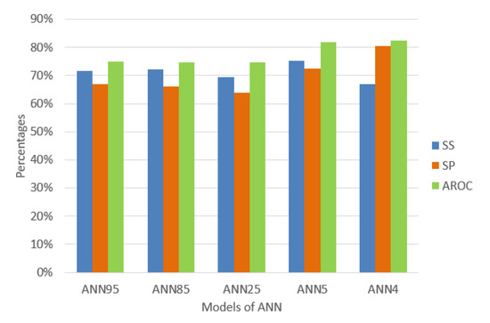
Figure 4.
Percentage of the performance indicators of the models of ANN.
The behavior of the data mining techniques shows in Figure 4 that the ANN of 4 hidden neurons is better compared to the previously proposed techniques. It appears that decreasing hidden neurons increases AROC, and this is a reason for some researchers to estimate hidden neurons empirically until the minimum number of neurons required is found. However, we decided to use a common method to calculate it [48,49,50] and had obtained promising results. The diagnostic of traditional MetS without doing a blood test presents an excellent level to discriminate (AROC = 82.48 %) using only four (4) variables AGE, WC, WHR, and SBP using an ANN of 4 hidden neurons. We found significant AROC values to determine an excellent MetS classification without using a blood sample and, at the same time, knowing which anthropocentric and clinical variables caused it.
However, based on clinical trials performed by the National Heart, Lung, and Blood Institute (NHLBI), excellent management of the individual risk factors of the syndrome should prevent or delay the onset of diabetes mellitus, hypertension, and cardiovascular disease [23,29,60].
MetS is a combination of five risk factors. For a MetS diagnosis, it is necessary to calculate the risk factors’ values according to the decision threshold shown in Table 1. An example case of MetS implies the combinations of the dichotomous variables represented by the format in base 2. This example case diagnoses MetS due to normal blood pressure, increased waist circumference, triglycerides, fasting plasma glucose and decreased HDL-C (W = 1, P = 0, G = 0, H = 1, and T = 1). Hence, the prevalence of W, P, G, H, and T in a dataset is significant for balancing each type of MetS. Therefore, we analyzed the percentage of W, P, G, H, and T, and the result was 72.68%, 27.97%, 13.33%, 63.58%, and 42.76%, respectively, as shown in Figure 5.
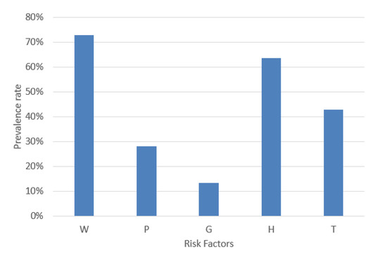
Figure 5.
Prevalence rate of the MetS risk factors.
3.3. Experiments to Diagnose Each MetS Type without a Blood Test
The experiments were performed based on the segmentation of MetS using the HMS criterion represented in Equation (6) that shows the ten (10) MetS types. We obtained these types by making an AND operation among each dichotomous risk factors W, P, G, H, and T using a dataset of 615 subjects, resulting in a distribution of the different (10) types of MetS shown in Figure 6 that shows the prevalence of each MetS type: WPT, WPH, WPG, WGT, WGH, WTH, PGH, PGT, PTH, and GHT were 14.31%, 16.75%, 5.53%, 7.32%, 9.11%, 26.18%, 3.9%, 3.9%, 10.41%, and 6.67%, respectively. These types are a built-in set giving the traditional MetS a prevalence rate of 42.60%.
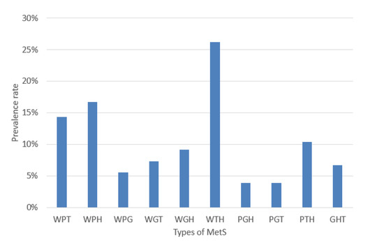
Figure 6.
Prevalence rate of the MetS types.
We can observe several MetS types with a low prevalence rate of less than 10%. We can note the risk factor (G) of fasting plasma glucose with the lowest rate (13.33%), as shown in Figure 5. This situation could lead to lower accuracy or AROC of prediction by the classifiers. The goal of the article is to classify each type of MetS. However, this research’s dataset is highly imbalanced, as depicted in Figure 6.
Therefore, we analyzed four approaches for improving the accuracy or AROC for the different MetS types due to an imbalance of the dataset.
- Approach 1 is using only the ANN technique with a feature selection algorithm.
- Approach 2 uses an ensemble classification algorithm in the dataset, which is the Random undersampling Boosted tree (RusBoost) ensemble.
- Approach 3 uses SMOTE to create more data that we called dataset with oversampling for then applying ANN.
- Approach 4 is using the dataset with oversampling and RusBoost.
For the approaches 1 and 3, we used for each MetS type a feed-forward Artificial Neural Network (ANN) with back-propagation of 3 layers perceptrons and with the training data (70% of the data) and the testing data (30% of the remaining data). For the validation, we used the random subsampling technique of 100 times.
It should be noted that approaches 1 and 2 used the original dataset of 615 samples, split into training and testing groups. However, approaches 3 and 4 used a dataset of 799 samples obtained using smote to create synthetic data and then splitting training or testing data.
3.3.1. Approach 1: Diagnosis of Each MetS Type Using the Original Dataset and ANN
We did the following to diagnose each MetS type without a blood test. We first selected the necessary features to achieve the maximum discrimination in the classification algorithms using a sequential feature selection algorithm in Matlab [58,59] using 17 variables. We obtained the set of variables detailed in Table 10. To compare the traditional or general MetS (MetSG) with the MetS types, we also show the features selected to build a model to diagnose it without a blood sample.
Table 10.
Selection of predicting variables for each MetS type from original dataset.
Table 10 shows the predictor variables for the MetS types. It is important to highlight the BFP variable’s relationship with the MetS types WPH, WGH, and WTH. This situation occurs due to the risk factor H (dichotomous HDL-C) dependence on gender. The MetS types related to P (dichotomous Blood Pressure) such as WPT, WPH, WPG, PGH, PGT, and PTH, according to the selection algorithm, have an evident relationship with the variables SBP and DBP. On the other hand, the MetS types WGT and GHT have the predictor variables WC and WSR, respectively, presenting a great challenge to discriminate them.
We then designed each classification model for the MetS, taking into account which variables would be treated. These selected features were used as inputs of the ANN with several hidden neurons calculated using Equation (9) as shown in Table 11 and with the same configuration parameter recommended by Kupusinac [33] to diagnose the following MetS types: WPG, WPH, WPT, WGT, WGH, WTH, PGT, PGH, PTH, and GHT according to the HMS criterion.
Table 11.
Numbers of hidden neurons from each ANN of the MetS types.
We validated each ANN using random subsampling, which we explained previously, obtaining the average performance indicators as shown Figure 7. The classification algorithms’ performance indicators for diagnosing the MetS type WPT show an outstanding ability to discriminate (AROC = 90.58%). Also, the diagnosis of the MetS type WPH has the same level of outstanding discrimination ability (AROC = 92.85%). The MetS type WPG diagnosis shows an excellent level to discriminate (AROC = 85.28%). The PGT and the PTH types also show an excellent level due to (AROC = 81.06%) and (AROC = 88.84%), respectively. The MetS type WGH, WTH, and PGH show an acceptable level (AROC = 71.93%), (AROC = 70.60%), and (AROC = 73.03%) respectively.
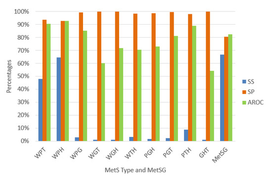
Figure 7.
Performance indicators of the ANN for the MetS types using the original dataset.
In contrast, for the diagnosis of the MetS types WGT, GHT, results show a substandard level of ability to discriminate (AROC = 60.13%), and (AROC = 54.13%) respectively. This situation is due to the low levels of sensitivity. A reason for this could be that there are so few predictive variables or low prevalence rates for each type, as shown in Figure 6. The figure shows that most of the MetS types have a prevalence rate of less than 10% and are affected or generated by the less prevalence rate of fasting plasma glucose of 13.33% compared to the other risk factors.
3.3.2. Approach 2: Diagnosis of Each MetS Type Using the Original Dataset and RusBoost
The approach 2 is to use the same variables’ selections of the dataset and an ensemble classification algorithm. The selected algorithm is the ensemble Random undersampling Boosted tree (RusBoost), which we explained previously. This classifier is appropriate for imbalanced data. We run RusBoost with the variables selections of Table 10 and with the configuration described by Table 5 to validate with random subsampling obtaining the average performance indicators given in Figure 8 that shows interestingly the RusBoost technique obtained excellent levels for the AROC performance indicator in the diagnosis of the MetS types WPT, WPH, WPG, PGH, PGT, and PTH. The values were 88.56%, 89.79%, 83.67%, 81.04%, 81.30%, and 83.33% respectively with improvements in sensitivity rate.
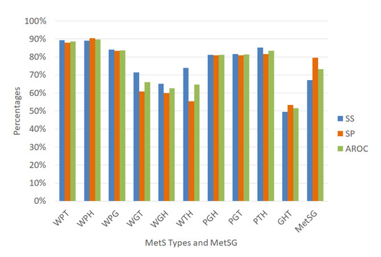
Figure 8.
Performance indicators of the RusBoost for the MetS types using the original dataset.
On the other hand, the results show lower AROC levels for the MetS types WGT, WGH, WTH, and GHT, with values of 66.11%, 62.58%, 64.71%, and 51.53%, respectively. For the MetS types WGT and GHT, their few predictors variables possibly affected the performance indicators. The same happened with other MetS types with a low prevalence of fasting plasma glucose that created this effect, generating an imbalance in the rest of the other data and affecting the AROC levels.
3.3.3. Approach 3: Diagnosis of Each MetS Type Using the Dataset with Oversampling and ANN
The approach 3 is to solve the imbalanced dataset for each MetS type. Several research articles have proposed that the balanced dataset improves prediction [61,62], and most importantly, it improves ANN training as the model can correctly adapt to the minority feature of the data. Therefore, we used the sampling methods technique to balance the dataset to improve the representation of each MetS type [63]. For this reason, a data balancing algorithm called SMOTE [41,42] was used with the WEKA data mining tool. In the dataset of 615 patients, the fasting plasma glucose dichotomous variable (G) was used in SMOTE to generate synthetic data [64] with a result of 799 samples (615 plus 184 synthetic data). This approach increased the prevalence of MetS to 51.81%, and improved the prevalence rate of fasting plasma glucose. It also updated the distribution of the W, P, G, H, and T risk factors. The new values were 73.72%, 29.16%, 30.79%, 65.58%, and 45.93%, respectively, as observed in Figure 9. We called the new dataset of 799 samples as dataset with oversampling.
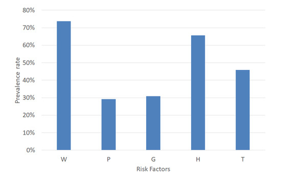
Figure 9.
Prevalence rate of the MetS risk factors using the dataset with oversampling.
Moreover, as a result of using SMOTE in the fasting plasma glucose (G) risk factor, the percentage of the MetS types related to fasting plasma glucose increased, as shown in Figure 10. This result shows that the prevalence rate of the MetS types WPG, WGT, and WGH is greater than 10%, PGH and PGT is greater than 5%, and GHT s higher than 15% in comparison with Figure 6. The prevalence rate of WPT, WPH, WPG, WGT, WGH, WTH, PGH, PGT, PTH, and GHT was 15.39%, 18.15%, 11.89%, 17.52%, 22.9%, 29.41%, 9.01%, 8.01%, 11.14%, and 15.39%, respectively. This result generated an increment in the prevalence rate of the traditional MetS of 51.81% as well.
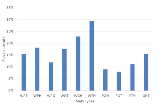
Figure 10.
Prevalence rate of the MetS types using the dataset with oversampling.
We used an algorithm of sequential feature selection from Matlab to achieve maximum discrimination in the classification algorithms, and Table 12 shows the results. This step refined the variables’ selection due to synthetic data’s creation, similar to the actual data. This step increments the positive values of the MetS types related to biochemical variables, especially those related to fasting plasma glucose. As part of this refinement, the types WPG and WGT selected POD as a predictor variable. On the other hand, the BFP variable remains in both Table 10 and Table 12, especially for the types WPH, WGH, and WTH. In those types, the biochemical variable HDL-C is related, and this depends on gender. The BFP variable is a function of gender, waist circumference, and age, demonstrating a logical relationship with WPH, WGH, and WTH types. Interestingly, the WPG and PGH types have the same initial predictor variables.
Table 12.
Selection of predicting variables for each target from the dataset with oversampling.
Afterward, we designed several ANN for each type of MetS according to the variables of Table 12 using the dataset with oversampling. These selected features were used as inputs of the ANN with several hidden neurons calculated using Equation (9) as shown in Table 13 and with the same configuration parameter recommended by Kupusinac [33] and was validated each ANN using random subsampling obtaining the average performance indicators as shown Figure 11.
Table 13.
Numbers of hidden neurons from each ANN of the MetS types.
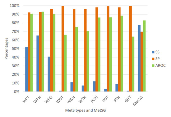
Figure 11.
Performance indicators of the ANN for the MetS types using the dataset with oversampling.
Figure 11 shows the ANN to classify for the diagnosis of the MetS types WPT, WPH, WPG were an outstanding ability to discriminate given that the AROC were 90.69%, 93.06%, and 90.57%, respectively with an excellent specificity rate. The MetS types PGH and PTH showed an excellent ability to discriminate AROC of 86.32% and 88.41%, respectively, with an excellent specificity rate. The PGT, WGH, and WTH types showed an acceptable level (AROC = 76.92%), (AROC = 75.52%), and (AROC = 70.38%) respectively, with a regular sensitivity rate.
In contrast, the diagnosis of the MetS types WGT and GHT showed a regular level (AROC = 66.22%) and (AROC = 64.06%), respectively. Moreover, the sensitivity rate was almost null due to the few positive cases that have that MetS type, generating overfitting in the ANN in the training stage, since it has learned more negative cases than positive ones. Therefore, these two models are not reliable in these conditions.
The prevalence of WGT and GHT is similar to the other MetS types that have an excellent level of AROC, such as WPT, WPH, WPG. Therefore, we think that the prevalence in this dataset with oversampling is not reason. However, the traditional MetS diagnosis improved its AROC level to 82.86% (Excellent)%.
3.3.4. Approach 4: Diagnosis of Each MetS Type Using the Dataset with Oversampling and RusBoost
Approach 4 uses the same variables selection from the dataset with oversampling of Table 12 and the ensemble Random undersampling Boosted tree (RusBoost) algorithm using the configuration described in Table 5 in the Methodology section to validate using random subsampling obtaining the average performance indicators given in Figure 12.
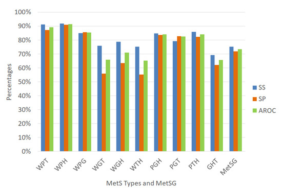
Figure 12.
Performance indicators of the RusBoost for the MetS types using the dataset with oversampling.
Figure 12 shows that the prediction accuracy values of the MetS types increased when compared with the results shown in Figure 8 and also the AROC discrimination ability values especially to diagnose the MetS type WGH due to obesity, high fasting plasma glucose, and low HDL-C with an acceptable level to discriminate (AROC = 71.08%) which increased 8.5%. The MetS type WPH showed an outstanding ability to discriminate with an AROC of 91.49% with an excellent sensitivity rate. The MetS types WPT, WPG, PGH, PGT, and PTH, showed an excellent ability to discriminate AROC 89.20%, 85.36%, 84.20%, and 84.10% respectively, with very good sensitivity rate. The MetS types WGH and PGT showed an acceptable level (AROC = 71.08%) and (AROC = 78.39%), respectively, with an acceptable sensitivity rate.
In contrast, the MetS types WGT, WTH, and GHT showed an regular level (AROC = 65.82%), (AROC = 65.16%), and (AROC = 65.65%), respectively. The prevalence of WGT, WTH, and GHT is similar to the other MetS types with an excellent level of AROC such as WPT, WPH, WPG.
4. Discussion
One important issue to discuss is the AROC low level for some of the MetS types. The AROC low level in the WGT, WTH, and GHT types is not related to the prevalence of each MetS type in the balanced dataset. However, the reason could be the few predictors variables of the models. On the other hand, it is interesting to note that when SMOTE is used to balance a risk factor such as fast plasma glucose in a dataset for traditional MetS diagnosis, minimal improvement in AROC levels is achieved. For ANN, the difference is 73.50% compared to 73.25%. For RusBoost, the difference is 82.48% compared to 82.86% using the same variables AGE, WC, WHR, and SBP.
Each medical organization established its criteria to diagnose the MetS, which varies according to the thresholds of risk factors. All the cited medical organizations have in common that for the diagnosis of the MetS, doctors must check at least three of five risk factors. Therefore, it is a combination of five risk factors, in which at least three are positive.
This article is an example of the conjunction of data science with the combinatorial analysis and the simplification applications by the Quine–McCluskey algorithm for finding the segmentation of the MetS. This approach achieved the diagnosis of the MetS types without using a blood sample that is, using a non-invasive method. For example, for a patient with waist circumference, triglycerides, and increased blood pressure, the system would predict only one type of MetS (WPT) to be active and the other types to be inactive. Therefore, doctors can infer that the patient has MetS due to increased triglycerides, blood pressure, and waist circumference to help focus on initial treatment and prevent diabetes mellitus or stroke.
We found that each MetS type’s predictor variables are different from those of the traditional MetS. These variables were used to configure each machine learning technique to diagnose each MetS type without a blood test. We also found that the prevalence of the MetS type related to the risk factor of fasting plasma glucose has a low rate. Therefore, we performed four approaches to improve the performance indicators of the classifiers.
The first approach was to use artificial neural networks to diagnose each of the MetS types working with previously selected variables, obtaining excellent AROC levels for the types of MetS such as WPG, WPT, WPH, WGH, WTH, PGT, PGH, and PTH. However, the sensitivity levels were low when diagnosing some MetS types indicating a high type 2 error level. The second approach was to use an algorithm specialized in data imbalance to compensate for the sensitivity levels and the specificity levels, thereby decreasing the ROC levels affecting four types of MetS WGT, WGH, WTH, and GHT.
The third approach was to increase the sample with an oversampling algorithm such as SMOTE, allowing evaluation of the ANN models with selected variables from these new data, finding an increase in AROC levels. However, the sensitivity levels are relatively low in some types, and so, the type 2 errors decreased relatively but are still high. The fourth approach was a mixture of using an imbalanced data prediction algorithm RusBoost with the larger dataset. We found a significant improvement in the levels of AROC for the MetS types levels and, at the same time, a considerable increase in sensitivity and, therefore, decreased the type 2 error. This result favored its choice compared to the neural networks for the types WPT, WPH, WPG, WGH, PGH, PGT, PTH. This approach resulted in 7 types of MetS that can be diagnosed without using a blood test. However, the types WGH, WTH, and GHT have a regular level to diagnose it, possibly due to the few predictors variables that can be reflected in its power of discrimination.
Another interesting point is that the MetS types WPT, WPH, WPG, PGH, PGT, PTH have better performance in the AROC than traditional MetS diagnosed using anthropometric variables using ANN or RusBoost.
The result of this article demonstrates the existence of ten (10) types of MetS according to the HMS criteria and their diagnostic using non-biochemical variables, such as the anthropometric and clinical variables using the ANN and RusBoost. Moreover, it demonstrates that doctors can diagnose traditional MetS using non-biochemical variables with classifiers. The results can vary according to the prevalence of the MetS types present in the dataset.
5. Conclusions
Healthcare professionals diagnose the Metabolic Syndrome through 5 factors, two of which they get in a medical consultation: Waist Circumference level (W) and blood pressure level (P). However, Triglyceride, HDL-C, and fasting plasma glucose levels (T, H, G) require a blood test. When we analyzed the segmentation of the MetS in types, we observed that for the diagnosis, an algorithm requires three risk factors, and we proved which risk factors generate that disease. Therefore, we suggest that in the future, MetS studies should take them into account to know which MetS type a patient has.
The present work uses information that doctors can collect from medical history and the medical visit. Such data includes Previous Obesity Diagnosis (POD), Age, Height, Weight (WG), Waist Circumference (WC), Hip Circumference (HC), Systolic and Diastolic Blood Pressure (SBP, DBP), Body Fat Percentage (BFP), and Body Mass Index. We used an algorithm of sequential feature selection and compared machine learning techniques such as ANN and RusBoost to diagnose the several types of MetS without doing a blood test. This discovery helps in an early screening of one or several MetS types through anthropometric and clinical data using non-invasive methods. From this point, doctors can take relevant actions to change them through habits modification.
We performed four approaches to obtain the best results. The first approach was carried out using clinical data from 615 subjects of selected variables to evaluate the ANN, obtaining excellent levels of AROC in the WPG, WPH, WPT, WGH, WTH, PGT, PGH, and PTH MetS types. However, the sensitivity levels were regular, presenting a considerable rate of type 2 errors due to the data imbalance. The second approach used a classifier for imbalanced data such as RusBoost, which improved the sensitivity levels to diagnose each MetS type, decreasing the type 2 error rate. However, the regular AROC levels decreased particularly for the classifiers for the WGT, WGH, WTH, and GHT types.
The third approach was to use the SMOTE technique to balance the data, and in this way, we achieved an improved performance of the ANN classifiers. However, in some classifiers, the sensitivity levels were regularly presenting a considerable rate of type 2 errors. The fourth approach was to use the balanced data and the RusBoost technique. This approach generated for the MetS types WPT, WPH, WPG, WGH, PGH, PGT, and PTH the following excellent AROC levels: 89.20%, 91.49%, 85.36%, 71.08%, 84.20%, 78.39%, and 84.10%, respectively, and with high sensitivity rates. The fourth approach obtained the best results for most MetS types, but for classifying the traditional MetS, the third approach was the best.
In the future, we plan to test the framework to diagnose the MetS types using an ANN model with ten output classification neurons (one for each type of MetS) as well as fuzzy logic, Bayesian networks, and other machine learning techniques.
Author Contributions
Conceptualization: M.B., E.N., M.J., and P.V.; formal analysis: M.B.; Methodology: M.B., and M.J.; software: M.B.; data curation: M.B., E.N., and P.V.; visualization: M.B., and M.J.; supervision: E.N., and P.V. All authors have read and agreed to the published version of the manuscript.
Funding
The first author received a Doctoral scholarship from the Administrative Department of Science, Technology, and Innovation—COLCIENCIAS of Colombia.
Acknowledgments
The first author expresses his deep thanks to the Administrative Department of Science, Technology, and Innovation—COLCIENCIAS of Colombia for the Doctoral scholarship. In addition, the author express their deep thanks to the Universidad del Norte and Universidad Autonoma del Caribe. The authors express their thanks to the reviewers of the article for their valuable comments and insights regarding the quality of the article.
Conflicts of Interest
The authors declare no conflict of interest.
Abbreviations
The following abbreviations are used in this manuscript:
| MDPI | Multidisciplinary Digital Publishing Institute |
| DOAJ | Directory of open access journals |
| IEEE | Institute of Electrical and Electronics Engineers |
| ACM | Association for Computing Machinery |
| DBLP | Digital Bibliography Library Project |
| GCP | Good Clinical Practices |
| ICH | Guide and the International Conference on Harmonization |
| WHO | World Health Organization |
| NCEP ATP III | National Cholesterol Education Programme Adult Treatment Panel III |
| EGIR | European Group for the study of Insulin Resistance |
| IDF | International Diabetes Federation |
| HMS | Harmonized Metabolic Syndrome |
| MetS | Metabolic Syndrome |
| MetSG | Metabolic Syndrome General |
| CHD | Coronary Heart Disease |
| IR | Insulin Resistance |
| ICD | International Classification of Diseases |
| OR | Odds Ratio |
| CI | Confidence Interval |
| SS | Sensitivity |
| SP | Specificity |
| FNR | False Negative Rate |
| FPR | False Positive Rate |
| AROC | Area under Receiver Operating Characteristic Curve |
| WC | Waist Circumference |
| BP | Blood Pressure |
| HDL-C | High-Density Lipoprotein Cholesterol |
| FPG | Fasting Plasma Glucose |
| TG | Triglycerides |
| WG | Weight |
| HG | Height |
| HC | Hip Circumference |
| WHHR | Waist to Hip ratio |
| WSR | Waist to Stature |
| BMI | Body Mass Index |
| BFP | Body Fat Percentage |
| SBP | Systole Blood Pressure |
| DBP | Diastole Blood Pressure |
| SBPD | Systole Blood Pressure Dichotomous |
| DBPD | Diastole Blood Pressure Dichotomous |
| W | Represents the normal(0) or raised(1) status of the dichotomous values of the WC |
| P | Represents the normal(0) or raised(1) status of the dichotomous variable of the BP |
| G | Represents the normal(0) or raised(1) status of the dichotomous variable of the FPG |
| H | Represents the normal(0) or lowed(1) status of the dichotomous variable of the HDL-C |
| T | Represents the normal(0) or raised(1) status of the dichotomous variable of the TG |
| ANN | Artificial Neural Networks |
| SMOTE | Synthetic Minority Oversampling Technique |
| PCLR | Principal Component Logistic Regression |
| RUSBoost | Random Undersampling Synthetic Minority Oversampling Technique |
Appendix A. Solution of Quine–McCluskey Algorithm to Minimize the MetS Types
The Quine–McCluskey algorithm aims to minimize the logical sum of products, which are the MetS types that we will call implicants. If the MetS type is a combination of 5 variables, it is represented in the algorithm as an implicant of order 0. If it is a combination of 4 variables, it would be of order 1, and if it is a combination of 3 variables, it would be of order 2.
- All those implicants of order 0, where only one variable has changed its state are grouped together. The group is obtained by eliminating the changed variable of those implicants of order 1. An example is the implicant of order 0, number 7 (W’P’GHT) and number 15 (W’PGHT), which are grouped together, resulting in W’GHT, which is of order 1.
- Then the implicants of order 1, where only one variable has changed its state are grouped together, obtained by eliminating changed variable. For example, the implicants 7, 15 (W’GHT) and 23, 31 (WGHT) (both implicants of order 1) are grouped together, resulting in GHT, which is of order 2.
- This process is carried out on all the implicants of order 0, until all implicants are minimized as shown Equation (6)
Table A1.
Implicants in the minimization of the MetS types.
Table A1.
Implicants in the minimization of the MetS types.
| IMPLICANTS | |||||
|---|---|---|---|---|---|
| n | Order 0 * | Order 1 | Order 2 | ||
| 7 | W’P’GHT | 7, 15 | W’GHT | 7, 15, 23, 31 | GHT |
| 11 | W’PG’HT | 7, 23 | P’GHT | 11, 15, 27, 31 | PHT |
| 13 | W’PGH’T | 11, 2 | W’PHT | 13, 15, 29, 31 | PGT |
| 14 | W’PGHT’ | 11, 3 | PG’HT | 14, 15, 30, 31 | PGH |
| 15 | W’PGHT | 13, 2 | W’PGT | 19, 23, 27, 31 | WHT |
| 19 | WP’G’HT | 3, 29 | PGH’T | 21, 23, 29, 31 | WGT |
| 21 | WP’GH’T | 14, 2 | W’PGH | 22, 23, 30, 31 | WGH |
| 22 | WP’GHT’ | 14, 30 | PGHT’ | 25, 27, 30, 31 | WPT |
| 23 | WP’GHT | 15, 31 | PGHT | 26, 27, 30, 31 | WPH |
| 25 | WPG’H’T | 19, 23 | WP’HT | 28, 29, 30, 31 | WPG |
| 26 | WPG’HT’ | 19, 27 | WG’HT | ||
| 27 | WPG’HT | 21, 23 | WP’GT | ||
| 28 | WPGH’T’ | 21, 29 | WGH’T | ||
| 29 | WPGH’T | 22, 23 | WP’GH | ||
| 30 | WPGHT’ | 22, 30 | WGHT’ | ||
| 31 | WPGHT | 23, 31 | WGHT | ||
| 25, 3 | WPG’T | ||||
| 25, 29 | WPH’T | ||||
| 26, 27 | WPG’H | ||||
| 26, 30 | WPHT’ | ||||
| 27, 31 | WPHT | ||||
| 28, 29 | WPGH’ | ||||
| 28, 30 | WPGT’ | ||||
| 29, 31 | WPGT | ||||
| 30, 31 | WPGH | ||||
* The symbol apostrophe (’) means that the variable is negative.
Appendix B
| Algorithm A1 RUSBoost Algorithm(Adapted from [65]). |
Given: Set S of examples ,..., with minority class Weak learner (decision tree), WeakLearn Number of iterations, T Desired percentage of total instances to be represented by the minority class, N
|
References
- Kaur, J. A Comprehensive Review on Metabolic Syndrome. Cardiol. Res. Pract. 2014, 1–21. [Google Scholar] [CrossRef]
- Cornier, M.-A.; Dabelea, D.; Hernandez, T.L.; Lindstrom, R.C.; Steig, A.J.; Stob, N.R.; Eckel, R.H. The Metabolic Syndrome. Endocr. Rev. 2008, 29, 777–822. [Google Scholar] [CrossRef] [PubMed]
- Müller-Nordhorn, J.; Willich, S.N. Coronary Heart Disease. In International Encyclopedia of Public Health, 2nd ed.; Academic Press: Cambridge, MA, USA, 2017; Volume 2, pp. 159–167. [Google Scholar] [CrossRef]
- WHO. Global Action Plan for the Prevention and Control of Noncommunicable Diseases 2013–2020; World Heal. Organ: Geneva, Switzerland, 2013; ISBN 978-9-24150-623-6. [Google Scholar]
- Navarro Lechuga, E.; Vargas Moranth, R. Metabolic syndrome in the southeast of Barranquilla (Colombia). Salud Uninorte 2008, 24, 40–52. [Google Scholar]
- Chobanian, A.V.; Bakris, G.L.; Black, H.R.; Cushman, W.C.; Green, L.A.; Izzo, J.L.; Roccella, E.J. Seventh Report of the Joint National Committee on Prevention, Detection, Evaluation, and Treatment of High Blood Pressure. Hypertension 2003, 42, 1206–1252. [Google Scholar] [CrossRef] [PubMed]
- Esposito, K.; Chiodini, P.; Colao, A.; Lenzi, A.; Giugliano, D. Metabolic Syndrome and Risk of Cancer: A systematic review and meta-analysis. Diabetes Care 2012, 35, 2402–2411. [Google Scholar] [CrossRef] [PubMed]
- Chen, J.; Muntner, P.; Hamm, L.L.; Jones, D.W.; Batuman, V.; Fonseca, V.; He, J. The Metabolic Syndrome and Chronic Kidney Disease in U.S. Adults. Ann. Intern. Med. 2004, 140, 167. [Google Scholar] [CrossRef] [PubMed]
- Grundy, S.M. Metabolic Syndrome: Connecting and Reconciling Cardiovascular and Diabetes Worlds. J. Am. Coll. Cardiol. 2006, 47, 1093–1100. [Google Scholar] [CrossRef]
- Grundy, S.M. Metabolic Syndrome Pandemic. Arterioscler. Thromb. Vasc. Biol. 2008, 28, 629–636. [Google Scholar] [CrossRef]
- Ford, W.H.; Giles, E.S.; Dietz, W.H. Prevalence of the Metabolic Syndrome Among US Adult. J. Am. Med. Assoc. 2002, 287, 356–359. [Google Scholar] [CrossRef]
- Mozumdar, A.; Liguori, G. Persistent Increase of Prevalence of Metabolic Syndrome Among U.S. Adults: NHANES III to NHANES 1999–2006. Diabetes Care 2011, 34, 216–219. [Google Scholar] [CrossRef]
- Aguilar, M.; Bhuket, T.; Torres, S.; Liu, B. Prevalence of the Metabolic Syndrome in the United States, 2003–2012. JAMA 2015, 313, 1973–1974. [Google Scholar] [CrossRef] [PubMed]
- Lakka, H. The Metabolic Syndrome and Total and Cardiovascular Disease Mortality in Middle-aged Men. JAMA 2002, 288, 2709–2716. [Google Scholar] [CrossRef] [PubMed]
- Grundy, S.M. Metabolic Syndrome: A Multiplex Cardiovascular Risk Factor. J. Clin. Endocrinol. Metab. 2007, 92, 399–404. [Google Scholar] [CrossRef]
- Aschner, P. Metabolic syndrome as a risk factor for diabetes. Expert Rev. Cardiovasc. Ther. 2010, 8, 407–412. [Google Scholar] [CrossRef]
- Gutiérrez-Solis, R.M.; Datta Banik, A.L.; Méndez-González, S. Prevalence of Metabolic Syndrome in Mexico: A Systematic Review and Meta-Analysis. Metabolic Syndrome and Related Disorders. Metab. Syndr. Relat. Disord. 2018, 16, 395–405. [Google Scholar] [CrossRef] [PubMed]
- Navarro, E.; Vargas, R.F. Coronary risk according to Framinghan equation in adults with metabolic syndrome in the city of Soledad, Atlantico, 2010. Rev. Colomb. Cardiol. 2012, 19, 109–118. [Google Scholar]
- Alberti, K.G.M.M.; Zimmet, P.Z. Definition, Diagnosis and Classification of Diabetes Mellitus and its Complications Part 1: Diagnosis and Classification of Diabetes Mellitus Provisional Report of a WHO Consultation. Diabet. Med. 1998, 15, 539–553. [Google Scholar] [CrossRef]
- Bartlett, J.G.M. Executive summary of the third report of the National Cholesterol Education Program (NCEP) expert panel on detection, evaluation and treatment of high blood cholesterol in adults. Infect. Dis. Clin. Pract. 2001, 10, 287–288. [Google Scholar]
- Balkau, B.; Charles, M. Comment on the provisional report from the WHO consultation. European Group for the Study of Insulin Resistance (EGIR). Diabet. Med. 1999, 16, 442–443. [Google Scholar]
- Alberti, K.G.M.M.; Zimmet, P.; Shaw, J. Metabolic syndrome—A new world-wide definition. A Consensus Statement from the International Diabetes Federation. J. Compil. 2006, 23, 469–480. [Google Scholar] [CrossRef]
- Alberti, K.G.M.M.; Eckel, R.H.; Grundy, S.M.; Zimmet, P.Z.; Cleeman, J.I.; Donato, K.A.; Smith, S.C. Harmonizing the Metabolic Syndrome International Atherosclerosis Society; and International Association for the Study of Obesity. Circulation 2009, 120, 1640–1645. [Google Scholar] [CrossRef] [PubMed]
- Minsalud. Informe Nacional de Calidad de la Atención en Salud 2015; Ministerio de Salud y Protección Social: Bogotá, Colombia, 2015; p. 217. [Google Scholar]
- Irving, G.; Neves, A.L.; Dambha-Miller, H.; Oishi, A.; Tagashira, H.; Verho, A.; Holden, J. International variations in primary care Doctor consultation time: A systematic review of 67 countries. BMJ Open 2017, 7, e017902. [Google Scholar] [CrossRef] [PubMed]
- Jover, A.; Corbella, E.; Mun, A.; Pedro-botet, J.; Herna, A.; Zu, M. Prevalence of Metabolic Syndrome and its Components in Patients With Acute Coronary Syndrome. Rev. EspañOla Cardiol. 2011, 64, 579–586. [Google Scholar] [CrossRef] [PubMed]
- De Kroon, M.L.; Renders, C.M.; Kuipers, E.C.; van Wouwe, J.P.; Van Buuren, S.; De Jonge, G.A.; Hirasing, R.A. Identifying metabolic syndrome without blood tests in young adults—The Terneuzen Birth Cohort. Eur. J. Public Health 2008, 18, 656–660. [Google Scholar] [CrossRef][Green Version]
- Hsiung, D.Y.; Liu, C.W.; Cheng, P.C.; Ma, W.F. Using non-invasive assessment methods to predict the risk of metabolic syndrome. Appl. Nurs. Res. 2015, 28, 72–77. [Google Scholar] [CrossRef]
- Alshehri, A. Metabolic syndrome and cardiovascular risk. J. Fam. Community Med. 2010, 17, 73. [Google Scholar] [CrossRef]
- Barrios, M.; Jimeno, M.; Villalba, P.; Navarro, E. Novel Data Mining Methodology for Healthcare Applied to a New Model to Diagnose Metabolic Syndrome without a blood test. Diagnostics 2019, 9, 192. [Google Scholar] [CrossRef]
- Murguía-Romero, M.; Jiménez-Flores, R.; Méndez-Cruz, A.R.; Villalobos-Molina, R. Predicting Metabolic Syndrome with Neural Networks. In Advances in Artificial Intelligence and Its Applications; Castro, F., Gelbukh, A., González, M., Eds.; Springer: Berlin/Heidelberg, Germany, 2013; pp. 464–472. [Google Scholar]
- Chen, H.; Xiong, S.; Ren, X. Evaluating the Risk of Metabolic Syndrome Based on an Artificial Intelligence Model. Abstr. Appl. Anal. 2014, 2014, 207268. [Google Scholar] [CrossRef]
- Ivanović, D.; Kupusinac, A.; Stokić, E.; Doroslovački, R.; Ivetić, D. ANN Prediction of Metabolic Syndrome: A Complex Puzzle that will be Completed. J. Med. Syst. 2016, 40, 264. [Google Scholar] [CrossRef]
- Navarro Lechuga, E.; Vargas Moranth, R.F.; Alcocer Olaciregui, A.E. Grasa corporal total como posible indicador de síndrome metabólico en adultos. Rev. EspañOla Nutr. Hum. DietéTica 2016, 20, 198. [Google Scholar] [CrossRef]
- Rodríguez, A.S.; Soidan, J.L.G.; Gómez, M.J.A.; Rodríguez, R.L.; del Alonso, A.Á.; Fernández, M.R.P. Metabolic syndrome and visceral fat in women with cardiovascular risk factor. Nutr. Hosp. 2017, 34, 863–868. [Google Scholar]
- Lean, M.E.J.; Han, T.S.; Deurenberg, P. Predicting body composition by densitometry from simple anthropometric measurements. Am. J. Clin. Nutr. 1996, 63, 4–14. [Google Scholar] [CrossRef] [PubMed]
- Fliotsos, M.; Zhao, D.; Rao, V.N.; Ndumele, C.E.; Guallar, E.; Burke, G.L.; Michos, E.D. Body mass index from Early-, Mid-, and Older-adulthood and risk of heart failure and atherosclerotic cardiovascular disease: MESA. J. Am. Heart Assoc. 2018, 7, e009599. [Google Scholar] [CrossRef] [PubMed]
- Floyd, T.L. Digital Fundamentals, 8th ed.; Pearson Education: New York City, NY, USA, 2002; ISBN 978-0130995278. [Google Scholar]
- Rosen, K.H. Discrete Mathematics and Its Applications, 5th ed.; McGraw-Hill Higher Education: New York, NY, USA, 2002. [Google Scholar]
- Perveen, S.; Shahbaz, M.; Keshavjee, K.; Guergachi, A. Metabolic Syndrome and Development of Diabetes Mellitus: Predictive Modeling Based on Machine Learning Techniques. IEEE Access 2019, 7, 1365–1375. [Google Scholar] [CrossRef]
- Chawla, N.V.; Bowyer, K.W.; Hall, L.O.; Kegelmeyer, W.P. SMOTE: Synthetic Minority Over-sampling Technique. J. Artif. Intell. Res. 2002, 16, 321–357. [Google Scholar] [CrossRef]
- Fernandez, A.; Garcia, S.; Herrera, F.; Chawla, N.V. SMOTE for Learning from Imbalanced Data: Progress and Challenges, Marking the 15-year Anniversary. J. Artif. Intell. Res. 2018, 61, 863–905. [Google Scholar] [CrossRef]
- Kumar, S. Neural Networks, 2nd ed.; Tata McGraw-Hill Education: New York, NY, USA, 2012. [Google Scholar]
- Bishop, C.M. Pattern Recognition and Machine Learning (Information Science and Statistics); Springer: Secaucus, NJ, USA, 2006. [Google Scholar]
- Hastie, T.; Tibshirani, R.; Friedman, J. The Elements of Statistical Learning (Second); Springer: New York, NY, USA, 2009. [Google Scholar] [CrossRef]
- Witten, I.H.; Frank, E. Data Mining: Practical Machine Learning Tools and Techniques, Second Edition (Morgan Kaufmann Series in Data Management Systems); Morgan Kaufmann Publishers Inc.: San Francisco, CA, USA, 2005. [Google Scholar]
- Andrea, T.A.; Kalayeh, H. Applications of Neural Networks m Quantitative Structure-Activity Relationships of Dihydrofolate Reductase Inhibitors. J. Med. Chem. 1991, 34, 2824–2836. [Google Scholar] [CrossRef]
- Boger, Z.; Guterman, H. Knowledge extraction from artificial neural networks models. In Proceedings of the IEEE International Conference on Systems, Man and Cybernetics, Orlando, FL, USA, 12–15 October 1997; pp. 3030–3035. [Google Scholar] [CrossRef]
- Karsoliya, S. Approximating Number of Hidden layer neurons in Multiple Hidden Layer BPNN Architecture. Int. J. Eng. Trends Technol. 2012, 3, 714–717. [Google Scholar]
- Panchal, F.S.; Panchal, M. Review on Methods of Selecting Number of Hidden Nodes in Artificial Neural Network. Int. J. Comput. Sci. Mob. Comput. 2014, 3, 455–464. [Google Scholar]
- Mounce, S.R.; Ellis, K.; Edwards, J.M.; Speight, V.L.; Jakomis, N.; Boxall, J.B. Ensemble Decision Tree Models Using RUSBoost for Estimating Risk of Iron Failure in Drinking Water Distribution Systems. Water Resour. Manag. 2017, 31, 1575–1589. [Google Scholar] [CrossRef]
- Seiffert, C.; Khoshgoftaar, T.M.; Van Hulse, J.; Napolitano, A. RUSBoost: Improving classification performance when training data is skewed. In Proceedings of the 2008 19th International Conference on Pattern Recognition, Tampa, FL, USA, 8–11 December 2008; pp. 1–4. [Google Scholar]
- Xu, Q.S.; Liang, Y.Z. Monte Carlo cross validation. Chemom. Intell. Lab. Syst. 2001, 56, 1–11. [Google Scholar] [CrossRef]
- Shao, J. Linear model selection by cross-validation. J. Stat. Plan. Inference 2005, 128, 231–240. [Google Scholar] [CrossRef]
- Fushiki, T. Estimation of prediction error by using K-fold cross-validation. Stat. Comput. 2011, 21, 137–146. [Google Scholar] [CrossRef]
- Berrar, D. Cross-Validation. In Encyclopedia of Bioinformatics and Computational Biology; Elsevier: Amsterdam, The Netherlands, 2019; pp. 542–545. [Google Scholar] [CrossRef]
- Hosmer, D.W.; Lemeshow, S. Assessing the Fit of the Model. In Applied Logistic Regression; John Wiley & Sons, Ltd.: Hoboken, NJ, USA, 2004; pp. 143–202. [Google Scholar] [CrossRef]
- Guyon, I.; Andre, E. An Introduction to Variable and Feature Selection. J. Mach. Learn. Res. 2003, 3, 1157–1182. [Google Scholar]
- Rückstieß, T.; Osendorfer, C.; van der Smagt, P. Sequential Feature Selection for Classification; Lecture Notes in Computer Science (Including Subseries Lecture Notes in Artificial Intelligence and Lecture Notes in Bioinformatics); Springer: Berlin/Heidelberg, German, 2011; pp. 132–141. [Google Scholar] [CrossRef]
- Duncan, G.E.; Perri, M.G.; Theriaque, D.W.; Hutson, A.D.; Eckel, R.H.; Stacpoole, P.W. Exercise Training, Without Weight Loss, Increases Insulin Sensitivity and Postheparin Plasma Lipase Activity in Previously Sedentary Adults. Diabetes Care 2003, 26, 557–562. [Google Scholar] [CrossRef]
- Bouwmeester, W.; Zuithoff, N.P.; Mallett, S.; Geerlings, M.I.; Vergouwe, Y.; Steyerberg, E.W.; Moons, K.G. Reporting and methods in clinical prediction research: A systematic review. PLoS Med. 2012, 9, e1001221. [Google Scholar] [CrossRef]
- Sun, Y.; Wong, A.K.C.; Kamel, M.S. Classification of imbalanced data: A review. Int. J. Pattern Recognit. Artif. Intell. 2009, 23, 687–719. [Google Scholar] [CrossRef]
- Melillo, P.; Luca, N.D.; Bracale, M.; Pecchia, L. Classification tree for risk assessment in patients suffering from congestive heart failure via long-term heart rate variability. IEEE J. Biomed. Heal. Inform. 2013, 17, 727–733. [Google Scholar] [CrossRef]
- Bolón-Canedo, V.; Sánchez-Maroño, N.; Alonso-Betanzos, A. A review of feature selection methods on synthetic data. Knowl. Inf. Syst. 2013, 34, 483–519. [Google Scholar] [CrossRef]
- Seiffert, C.; Khoshgoftaar, T.M.; Van Hulse, J.; Napolitano, A. RUSBoost: A Hybrid Approach to Alleviating Class Imbalance. IEEE Trans. Syst. Man Cybern. Part A Syst. Hum. 2020, 40, 185–197. [Google Scholar] [CrossRef]


Publisher’s Note: MDPI stays neutral with regard to jurisdictional claims in published maps and institutional affiliations. |
© 2020 by the authors. Licensee MDPI, Basel, Switzerland. This article is an open access article distributed under the terms and conditions of the Creative Commons Attribution (CC BY) license (http://creativecommons.org/licenses/by/4.0/).