Featured Application
Existing camera systems may provide localization and tracking of everything marked, while AGVs do not have to carry sensors for localization and navigation themselves. This method provides centralized supervision of deployed robotic systems.
Abstract
The objective of this study is to extend the possibilities of robot localization in a known environment by using the pre-deployed infrastructure of a smart building. The proposed method demonstrates a concept of a Shared Sensory System for the automated guided vehicles (AGVs), when already existing camera hardware of a building can be utilized for position detection of marked devices. This approach extends surveillance cameras capabilities creating a general sensory system for localization of active (automated) or passive devices in a smart building. The application is presented using both simulations and experiments for a common corridor of a building. The advantages and disadvantages are stated. We analyze the impact of the captured frame’s resolution on the processing speed while also using multiple cameras to improve the accuracy of localization. The proposed methodology in which we use the surveillance cameras in a stand-alone way or in a support role for the AGVs to be localized in the environment has a huge potential utilization in the future smart buildings and cities. The available infrastructure is used to provide additional features for the building control unit, such as awareness of the position of the robots without the need to obtain this data directly from the robots, which would lower the cost of the robots themselves. On the other hand, the information about the location of a robot may be transferred bidirectionally between robots and the building control system to improve the overall safety and reliability of the system.
1. Introduction
Imagine that in the future every building will look like a living organism comparable to a hive where both humans, robots, and other devices are going to cooperate on their tasks. For example, mobile robotic systems will assist people with basic repetitive tasks, such as package and food delivery, human transportation, security, cleaning, and maintenance. Besides fulfilling the purpose, robots need to be safe for any person that comes in contact with one, so any possible harm is avoided. A robot position tracking and collision avoidance plays a key role to ensure such capabilities.
There are many methodologies for motion planning and their theoretical approaches are described in a survey by Mohanan and Salgoankar [1]. One of the most used methods is Simultaneous Localization and Mapping (SLAM) [2] where the environment is not known, so a vision based system is placed on a robot to observe the area and create a map of it, eventually to perform trajectory planning on top of it. There were many enhancements of the SLAM methods proposed, some of them are compared by Santos [3] and the most common sensors used there are lidars [4,5,6,7] and depth cameras [4,8,9,10]. However, when the environment is known (indoor areas frequently), the advanced SLAM systems may become redundant and if more robots are deployed, it becomes costly when every single robot has to carry all sensors.
Therefore, some alternatives come to mind, such as real-time locating systems (RTLS), when devices working on the radio frequency communication principle are placed in the environment to determine the position of a robot. Under this technology, one can imagine WiFi [11,12], when time-difference measurements between the towers and the monitored object are obtained, or RFID [13,14,15], when tags shaped in a matrix on the floor or walls are detected by a transmitter on the robot. However, deployment of RTLS is not always possible, when WiFi needs uninterrupted visual contact and reliable communication between the towers. The RFID tags on the floor can be damaged during a time and the accuracy is based on the density (amount) of the tags. In general, RTLS is suitable only for indoor areas. On the other hand, the most common GNSS systems for outdoor navigation cannot provide a reliable solution in the case of indoor environments.
Another approach for robot navigation is odometry, which analyzes the data from onboard sensors and estimates the position change over time. Mostly the wheel encoders are used [16], or a camera for visual odometry [17]. Although, the odometry measurements have a disadvantage when they accumulate an error with time, as investigated by Ganganath [18], where he proposed a solution using a Kinect sensor that is detecting tag markers placed in the environment. Similar methods of robot localization when the map is known and visual markers are deployed are presented in [19,20]. The other possible solution of an object localization is a marker-based motion capture system, in which the functioning with multiple robots was demonstrated in [21], but only a single camera was used and all paper-printed markers were the same, so it is not possible to use it for device identification. Infra-red markers have a similar disadvantage, they were used for tracking AGVs with either a number of high-speed cameras in [22,23,24] or the Kinect system in [25]. When many robots at the same place are used, a field Swarm Robotics [26] comes to mind. Some algorithms tested with real robots were introduced [27,28], but they were not applied on different types of robots and have not been tested in cooperation with humans or in an environment where people randomly appear and disappear.
Except for the RTLS and motion capture, the previously mentioned methods are based on sensor systems carried by a robot. Furthermore, only the robot determines its pose and in case of an unexpected situation, it might lead to a fault state and connection lost without providing any reliable feedback to the control system of a building, as shown in Figure 1a. The RTLS avoid this situation, but only because of added devices such as communication towers. The marker-based motion capture system, if used in common areas like rooms and corridors of a building, needs many cameras deployed and a specific pattern of IR markers on every device. If there are tens or hundreds of devices, to define and to recognize the markers becomes a difficult task. However, smart buildings may already have their sensor systems, mostly cameras and related devices for security purposes. Nowadays, face-recognition and object detection software has been used in airports [29], governmental buildings, other public places, and even in smart phones. These capabilities lead us to an approach when the surveillance cameras would be involved in the facial recognition and tracking of any robot or device at the same time, meaning that every device has its unique easily printable marker that characterizes it, so the control system of the whole building has an independent feedback on a device’s pose continuously. This also extends the possibility of tracking things in an environment even though they are not electronic devices, for example important packages and boxes. Such a solution acts, as we call it, as a Shared Sensory System. This approach simplifies the tracking of new devices, as only their ID is needed, as well as a new marker to be placed on a device or thing to the control system.
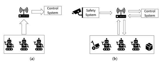
Figure 1.
A robot pose determination: (a) Nowadays robots inform control systems about their pose; (b) Proposed method of determination of any device pose, robots may provide their own pose estimation so two-way detection is performed.
Furthermore, the hardware costs are minimized when the devices do not need to carry any computational units or sensors. The image analysis, object detection, localization, and trajectory planning of AGVs may run in the cloud. The scheme of the system is shown in Figure 1b.
2. Test Benches and Methods
There are more options of detecting an object in an image as compared to a survey of Parekh [30]. For image processing and tag marker detection we used OpenCV library [31] and methodology described in [32] for detecting an Aruco 3D gridboard, which improves the reliability and accuracy of the detection in comparison with basic 2D tags. The gridboard (Figure 2) represents a coordinate frame and may be placed on a robot.
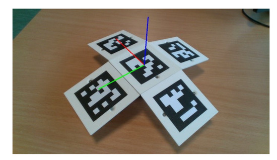
Figure 2.
Aruco 3D gridboard with detected coordinate frame XYZ—red, green, blue, respectively.
The OpenCV Aruco module analyzes an image from a camera and calculates the transformation from a tag to the camera. This transformation is represented by a homogenous transformation matrix, including the position and rotation of the detected coordinate frame. Every unique marker may represent a unique robot or device. When there are more of them placed in the field of view of a camera, the transformation between them is calculated directly, or in reference to the base coordinate frame. The homogenous transformation matrix from a global coordinate frame (base frame B) to the robot frame is calculated by Equation (1). The is a known transformation from the global coordinate frame to the camera frame. The is the detected transformation from the camera frame to the robot frame, obtained from image processing. The transformation matrices, in terms of robot kinematics, are described by Legnani [33].
We assume that the placements of all cameras are known, the transformations between the cameras may be determined by their layout related to a world coordinate frame. With this information, it is possible to track and calculate the positions between tagged objects even if they are in different parts of a building. Number of cameras has an impact on the accuracy of the detection, as it is described in Section 3. Results show, however, that even a single camera provides reliable data on the location of an AGV. To demonstrate the difference between the number of cameras used, we designed a camera system with 3 cameras of the same type, which is shown in Figure 3 schematically and in Figure 4 as captures of simulation. Finally, the same system was deployed in the experiment, which is shown in Figure 5. Fields of view of those cameras intersect and are described in Figure 3. Such a system might serve, for example, as a face-recognition every time a human wants to enter a door. If this person is allowed to enter, the door can automatically unlock and open, which may be appreciated in clean rooms, such as biomedical labs, where, for example, samples of dangerous diseases are analyzed. Our methodology utilizes these kinds of cameras for AGVs localization and makes them multipurpose.
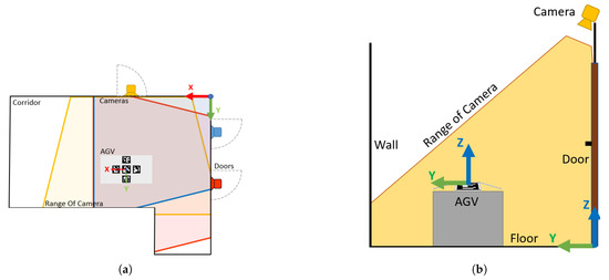
Figure 3.
Schematics of cameras placement: (a) top view; (b) side view.
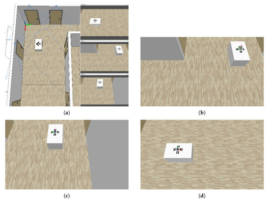
Figure 4.
Simulation environment: (a) top view; (b) red camera view; (c) blue camera view; (d) yellow camera view. Resolution for every camera was set to 1280 × 720 px this time.
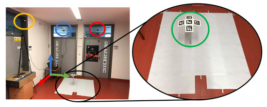
Figure 5.
Real test: the cameras are highlighted with yellow, blue, and red circles. The gridboard is in a green circle representing the position of an automated guided vehicles (AGV).
2.1. Simulation with Single Robot
The concept was simulated and tested in an environment similar to that described in the previous chapter and as shown in Figure 4a. The cameras were deployed above the doors in a corridor. In the simulation, an AGV position was represented as a box with a 3D gridboard on top of it. The robot was moving along a trajectory loop under the cameras. The results of this simulation are supposed to provide an idea about how accurate the detection can be if the environmental conditions (sun light, reflections, artificial lightning, etc.) are ideal, secondly what impact the cameras resolution has on the detection. The crucial outcome is the comparison between accuracy and processing time when resolution differs. As the processing time, we understand the period when the OpenCV algorithm is analyzing an image that was previously captured and stored in a buffer as the most recent. The average processing time depends on the number of pixels and stays the same no matter if an analyzed image was captured in the simulation or real test.
In Figure 4b–d, the images captured by all three cameras at the same time can be seen. The images were already processed, so the coordinate frame of the detected tag is visible. The resolution has an impact on a tag detection—higher resolution may detect a smaller (more distant) marker. The simulated resolutions for the chosen tags with dimensions of 70 × 70 mm were:
- 1920 × 1080 px
- 1280 × 720 px
- 640 × 480 px
2.2. Experiment
Based on the simulation result we performed the real test, as shown in Figure 5. The objective of the experiment was to determine the absolute accuracy of the detection. Therefore, the gridboard was placed on a static rod, which allowed us to check the detected position with its absolute value that was measured using a precisely placed matrix of points on the floor (white canvas in Figure 5). The rod was moved into 14 different positions, which were 250 mm apart from each other. In every position, 40 measurements were taken for a dataset that was analyzed later. The height of the gridboad above the floor on the simulated robot was the same as the height of the gridboard on the rod in the experiment, 460 mm exactly. The cameras were 2500 mm above the floor. Resolution was set to 1280 × 720 px for the cameras in the experiment when it provided the best performance in the simulation, as described in the Results Section. The control PC was running on Ubuntu 16.04 with a CPU of 4 cores at 2.80 GHz, the USB 3 was providing connection to the Intel D435i [34] depth cameras; however, only their RGB image was analyzed. It is important to note that camera calibration process is crucial for the accuracy of the detection, as it is described in [35]. The cameras were calibrated following these instructions.
In both simulation and experiment, the relation between the number of cameras and the detected position accuracy was examined.
For presenting the accuracy results of this method, we chose to determine the absolute distance from the point where a tag’s coordinate frame was expected to the point where it was measured. Only X and Y coordinates were considered, the Z coordinate is known for every robot—the height of a tag in our case. In Equation (2), the calculated accuracy error is presented. The and represent the expected values, the and represent the measured coordinates by a camera.
In the simulation and experiment, only the position values X and Y of the gridboard were later analyzed and presented in the Results Section. However, during the image processing, all data as position values and values for orientation were acquired.
2.3. Simulation with Multiple Robots
The purpose of the second simulation is to present the capabilities of our algorithm to detect multiple robots using multiple cameras. The trajectories and lookout of the robots are shown in Figure 6. The tags on the black robot were placed at different positions in comparison with the white robot, but the system can handle this. In comparison with the first simulation, the size of the tags was changed to 170 × 170 mm to highlight the scalability of the system. At some point of the simulation the robots are detected by one or more cameras and at another point both robots are detected by all cameras. The environment and camera position stayed the same as in the previous simulation with a single robot. The 1280 × 720 px camera resolution was used. The simulation step was set to = 0.0333 s, which corresponds to 30 fps, which is a general value for most of the cameras. Based on this setup, the velocity of the robot was calculated as the change of the position in two captured frames in time, as shown in Equation (3). The represent the position of a robot in frame, the represent the position of the robot in the previous frame.
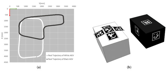
Figure 6.
Multiple robots simulation: (a) trajectories of the robots in the previously described environment; (b) marked robots, the size of the tags was set to 170 × 170 mm.
The default speed of the robots was set to 1.5 m/s in the simulation, the error between this value and the calculated velocity v based on the marker detection is presented in the Results Section.
A video with an additional description of the simulation of multiple robots was uploaded on a YouTube channel [36] of the Department of Robotics, VSB-TU of Ostrava. A Python source code of the detection is available as a Github repository [37].
3. Results
In the case of the simulation with a single robot, we present data on the detection accuracy error for the three resolutions in Figure 7a, when the image from a single camera was used. The zero value of the graph represents the real position of the robot, measured by the CoppeliaSim simulation engine, where it is possible to read the absolute position data of every object. As expected, with a smaller resolution of a camera the accuracy drops down. However, the difference between Full HD and HD image resolution is only 4.8 mm on average. In addition, when observing the processing time for an image in Figure 7b the HD resolution may provide twice as fast detection as Full HD.
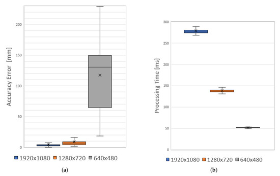
Figure 7.
Simulation results: (a) detection accuracy error; (b) processing time.
The simulation results with the single robot are presented in Table 1. The data show the relation between the resolution of a camera and its impact on detection accuracy and processing time. The accuracy can be influenced by many aspects, but the processing time of an image is very closely related to the number of pixels. Therefore, in the following real cameras experiment, 1280 × 720 px resolution was used when it provides (observing Table 1) good performance between accuracy and processing time.

Table 1.
Average accuracy and processing time of detection in simulation.
More cameras can detect a gridboard all at once. In this simulation and experiment, we detected it with one, two or three cameras to compare the results. An average value of the position vector for two or three cameras was determined. In Figure 8 there is a comparison of the position accuracy error for single or multiple cameras. As shown in Figure 8b for the experiment, when more cameras were used, the absolute error was not improved significantly; however, the variance of the error was lowered. The reason why the error does not go down substantially when more cameras are used is that at a random position the robot appears in different areas of the images of every camera. In the center of an image, the localization is the most precise, in the sides of an image, the precision of detection is decreasing. This effect is described later in Figure 9.
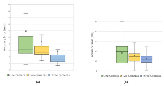
Figure 8.
Comparison of detection when one, two or three cameras were used: (a) simulation; (b) experiment.
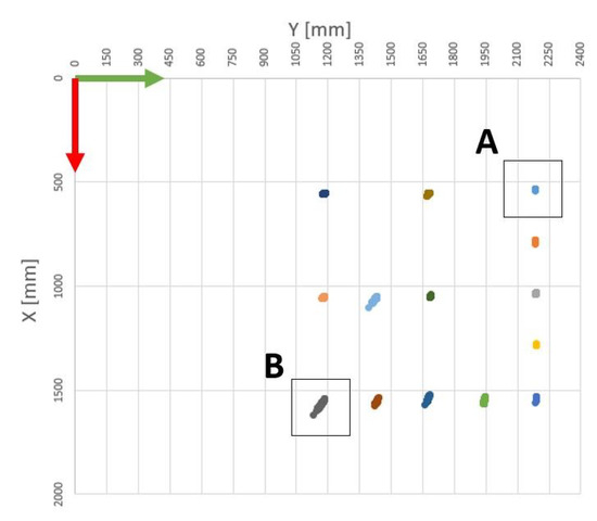
Figure 9.
Detection accuracy of a single camera in a real experiment. Every color represents a different set of measured positions. It is the red camera in Figure 5, specifically.
The average values of the accuracy error in the simulation with the single robot and experiment presented in Figure 8 are stated in Table 2.
Table 2.
Comparison of average accuracy error of detection in simulation with the single robot vs. real test.
Figure 9 represents the distortion [35] of nonperfect calibration of a camera. Therefore, more cameras cannot guarantee the absolute accuracy of the detection; on the other hand, the error can be significantly lowered when there two or more cameras are used. In Figure 9, the 14 different positions were measured 40 times by a camera highlighted by the red circle in Figure 5. The set of points A with mm was very close to the center of the camera’s field of view. The set of points B was the most distant and the dispersion of the 40 measurements is the most significant.
The following graphs are the results of the simulation with multiple robots. In Figure 10, the accuracy of the algorithm is presented, comparing the defined path of the robots and the detected path.
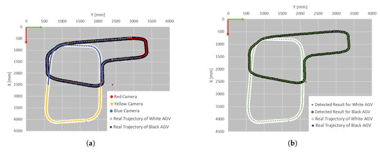
Figure 10.
Comparison of detected and real positions during the simulation with multiple robot: (a) results for every camera; (b) average value.
The graphs of Figure 10 prove excellent general accuracy of the system. The results are overlapping with the absolute position values measured by the simulation engine and the difference is not clearly visible in this scale. Therefore, in Figure 11 the error values of the detected X and Y coordinates are presented. Zero error means that the detected position is equal to the real position of the robot. The colors of lines represent the cameras and the dashed line is the average value. There is no smoothing filter applied on the data, some peak values are visible. The application of filtering is one of the subjects for the future research.
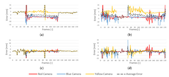
Figure 11.
Error between detected and real position of the robots: (a) X direction of white robot; (b) X direction of black robot; (c) Y direction of white robot; (d) Y direction of black robot.
The obtained data may be analyzed for other purposes, for example, in the graphs of Figure 12 the speed of the robots was calculated based on the difference between the positions in time, comparing and frames. In the simulation for multiple robots, 175 frames were obtained in total.
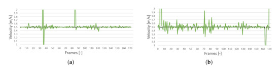
Figure 12.
Calculated velocity of robots: (a) white robot; (b) black robot.
4. Conclusions
In addition to the previous chapter where the results were presented, some other ideas and relations to the research of others may be discussed here. This study shows how the hardware that is already deployed may be used for another purpose in the case of smart cities and buildings, when only a software module with a control unit is added. The only prerequisite is having access to real-time image data of the installed camera system and computing capabilities for image processing, which can be run locally or in the cloud. In general, the price of a smart building is already high, and it increases with every added technology. This approach may lead to lower cost and create a Shared Sensory System for all AGVs at the level of a whole building and surrounding area.
We presented a possible use case when images of face-recognition security cameras, which were placed above the doors to provide automatic unlocking and opening, were also used for tracking of robots and other devices. This method can be applied to a robot navigation adding algorithm [38] for human and object detection of autonomous cars. Such capabilities would allow to stop or slow down a robot when a person is approaching while hidden behind a corner, so the human is not in the robot’s field of view. Alternatively, the methodology may be used along with SLAM to add another safety feature to the control system.
The choice of camera resolution has an influence on the reliability and processing time of the system. In our measurements, for the real-time tracking application, the 640 × 480 px resolution would be necessary, but the drop in the case of accuracy might be a problem. However, the processing time may be solved if more powerful control PC is used. In the experiment, we used resolution 1280 × 720 px, which provided the best ratio between accuracy and speed of localization for us. When more cameras are deployed, a higher computing power is demanded. Therefore, more processing units or cloud computing for analyzing the images should be considered. Another disadvantage of the system is that a device position might be lost if it is not detected by any camera. In this case, the control system should be prepared for dealing with such a situation. For example, the robot shall be stopped until allowed to continue in its trajectory or reset.
For the most accurate detection of a tag, every camera should be calibrated. On the other hand, if many cameras of the same type are deployed, the calibration constants can be determined statistically performing the calibration with a few of these cameras and distributing the calibration file with constants of average values. If a new camera is added to the system, its precise position can be determined using an additional device with tag markers placed at a certain distance from the camera using the device’s known dimensions.
In multiple camera detection, we use a simple distance average for the detected objects. Another approach to determine the position more accurately is to apprise the distance of every camera to the detected object. Therefore, the nearest camera that should provide the most precise detection would obtain a higher weight than the others. This is a topic for further research.
Our algorithm can deal with multiple marker detection. This can be deployed whenever in a building with coverage of the camera’s field of view and used for localization of any device with the marker, not only robots. In addition to that, this system could be applied in the outdoor environment using the surveillance camera systems deployed by governments. For example, in the case of the possibility of using the image data, car-sharing or autonomous taxi companies could place unique markers on the roofs of their vehicles fleet, and the position of a vehicle could be inquired in the governmental system, which might be an additional benefit for a public city.
Author Contributions
Conceptualization, P.O. and D.H.; methodology, Z.B. and P.O.; software, P.O.; validation, J.B. and Z.B.; formal analysis, V.K., D.H. and P.O.; investigation, Z.B. and J.B.; resources, D.H., V.K. and J.B.; data curation, P.O. and J.B.; writing—original draft preparation, D.H. and P.O.; writing—review and editing, D.H.,V.K. and Z.B.; visualization, P.O., D.H.,V.K. and J.B.; supervision, Z.B.; project administration, V.K. and Z.B.; funding acquisition, V.K. and Z.B. All authors have read and agreed to the published version of the manuscript.
Funding
This work was supported by the Research Platform focused on Industry 4.0 and Robotics in Ostrava Agglomeration project, project number CZ.02.1.01/0.0/0.0/17_049/0008425 within the Operational Programme Research, Development and Education. This article has also been supported by a specific research project SP2020/141 and financed by the state budget of the Czech Republic.
Conflicts of Interest
The authors declare no conflict of interest. The funders had no role in the design of the study; in the collection, analyses, or interpretation of data; in the writing of the manuscript, or in the decision to publish the results.
Abbreviations
The following abbreviations are used in this manuscript:
| AGV | Automated Guided Vehicle |
| FPS | Frames per Second |
| GNSS | Global Navigation Satellite System |
| OpenCV | Open Source Computer Vision Library |
| RFID | Radio Frequency Identification |
| RGB | Red Green Blue |
| RTLS | Real Time Locating System |
| SLAM | Simultaneous Localization and Mapping |
References
- Mohanan, M.; Salgoankar, A. A survey of robotic motion planning in dynamic environments. Robot. Auton. Syst. 2018, 100, 171–185. [Google Scholar] [CrossRef]
- Montemerlo, M.; Thrun, S.; Koller, D.; Wegbreit, B. FastSLAM: A factored solution to the simultaneous localization and mapping problem. Aaai/iaai 2002, 593–598. [Google Scholar]
- Santos, J.M.; Portugal, D.; Rocha, R.P. An evaluation of 2D SLAM techniques available in Robot Operating System. In Proceedings of the 2013 IEEE International Symposium on Safety, Security, and Rescue Robotics (SSRR), Linkoping, Sweden, 21–26 October 2013. [Google Scholar] [CrossRef]
- Pandey, G.; McBride, J.R.; Eustice, R.M. Ford Campus vision and lidar data set. Int. J. Robot. Res. 2011, 30, 1543–1552. [Google Scholar] [CrossRef]
- Blanco-Claraco, J.L.; Moreno-Dueñas, F.Á.; González-Jiménez, J. The Málaga urban dataset: High-rate stereo and LiDAR in a realistic urban scenario. Int. J. Robot. Res. 2013, 33, 207–214. [Google Scholar] [CrossRef]
- Li, L.; Liu, J.; Zuo, X.; Zhu, H. An Improved MbICP Algorithm for Mobile Robot Pose Estimation. Appl. Sci. 2018, 8, 272. [Google Scholar] [CrossRef]
- Olivka, P.; Mihola, M.; Novák, P.; Kot, T.; Babjak, J. The Design of 3D Laser Range Finder for Robot Navigation and Mapping in Industrial Environment with Point Clouds Preprocessing. In Modelling and Simulation for Autonomous Systems; Springer International Publishing: Berlin/Heidelberg, Germany, 2016; pp. 371–383. [Google Scholar] [CrossRef]
- Biswas, J.; Veloso, M. Depth camera based indoor mobile robot localization and navigation. In Proceedings of the 2012 IEEE International Conference on Robotics and Automation, Saint Paul, MN, USA, 14–18 May 2012. [Google Scholar] [CrossRef]
- Cunha, J.; Pedrosa, E.; Cruz, C.; Neves, A.J.; Lau, N. Using a Depth Camera for Indoor Robot Localization and Navigation; DETI/IEETA-University of Aveiro: Aveiro, Portugal, 2011. [Google Scholar]
- Yao, E.; Zhang, H.; Xu, H.; Song, H.; Zhang, G. Robust RGB-D visual odometry based on edges and points. Robot. Auton. Syst. 2018, 107, 209–220. [Google Scholar] [CrossRef]
- Jachimczyk, B.; Dziak, D.; Kulesza, W. Using the Fingerprinting Method to Customize RTLS Based on the AoA Ranging Technique. Sensors 2016, 16, 876. [Google Scholar] [CrossRef] [PubMed]
- Denis, T.; Weyn, M.; Williame, K.; Schrooyen, F. Real Time Location System Using WiFi. Available online: https://www.researchgate.net/profile/Maarten_Weyn/publication/265275067_Real_Time_Location_System_using_WiFi/links/54883ed60cf2ef3447903ced.pdf (accessed on 11 November 2020).
- Kulyukin, V.; Gharpure, C.; Nicholson, J.; Pavithran, S. RFID in robot-assisted indoor navigation for the visually impaired. In Proceedings of the 2004 IEEE/RSJ International Conference on Intelligent Robots and Systems (IROS) (IEEE Cat. No.04CH37566), Sendai, Japan, 28 September–2 October 2004. [Google Scholar] [CrossRef]
- Chae, H.; Han, K. Combination of RFID and Vision for Mobile Robot Localization. In Proceedings of the 2005 International Conference on Intelligent Sensors, Sensor Networks and Information Processing, Melbourne, Australia, 5–8 December 2005. [Google Scholar] [CrossRef]
- Su, Z.; Zhou, X.; Cheng, T.; Zhang, H.; Xu, B.; Chen, W. Global localization of a mobile robot using lidar and visual features. In Proceedings of the 2017 IEEE International Conference on Robotics and Biomimetics (ROBIO), Macau, China, 5–8 December 2017. [Google Scholar] [CrossRef]
- Chong, K.S.; Kleeman, L. Accurate odometry and error modelling for a mobile robot. In Proceedings of the International Conference on Robotics and Automation, Albuquerque, NM, USA, 25 April 1997. [Google Scholar] [CrossRef]
- Scaramuzza, D.; Fraundorfer, F. Visual Odometry [Tutorial]. IEEE Robot. Autom. Mag. 2011, 18, 80–92. [Google Scholar] [CrossRef]
- Ganganath, N.; Leung, H. Mobile robot localization using odometry and kinect sensor. In Proceedings of the 2012 IEEE International Conference on Emerging Signal Processing Applications, Las Vegas, NV, USA, 12–14 January 2012. [Google Scholar] [CrossRef]
- Ozkil, A.G.; Fan, Z.; Xiao, J.; Kristensen, J.K.; Dawids, S.; Christensen, K.H.; Aanaes, H. Practical indoor mobile robot navigation using hybrid maps. In Proceedings of the 2011 IEEE International Conference on Mechatronics, Istanbul, Turkey, 13–15 April 2011. [Google Scholar] [CrossRef]
- Farkas, Z.V.; Szekeres, K.; Korondi, P. Aesthetic marker decoding system for indoor robot navigation. In Proceedings of the IECON 2014-40th Annual Conference of the IEEE Industrial Electronics Society, Dallas, TX, USA, 29 October–1 November 2014. [Google Scholar] [CrossRef]
- Krajník, T.; Nitsche, M.; Faigl, J.; Vaněk, P.; Saska, M.; Přeučil, L.; Duckett, T.; Mejail, M. A Practical Multirobot Localization System. J. Intell. Robot. Syst. 2014, 76, 539–562. [Google Scholar] [CrossRef]
- Goldberg, B.; Doshi, N.; Jayaram, K.; Koh, J.S.; Wood, R.J. A high speed motion capture method and performance metrics for studying gaits on an insect-scale legged robot. In Proceedings of the 2017 IEEE/RSJ International Conference on Intelligent Robots and Systems (IROS), Vancouver, BC, Canada, 24–28 September 2017. [Google Scholar] [CrossRef]
- Qin, Y.; Frye, M.T.; Wu, H.; Nair, S.; Sun, K. Study of Robot Localization and Control Based on Motion Capture in Indoor Environment. Integr. Ferroelectr. 2019, 201, 1–11. [Google Scholar] [CrossRef]
- Bostelman, R.; Falco, J.; Hong, T. Performance Measurements of Motion Capture Systems Used for AGV and Robot Arm Evaluation. Available online: https://hal.archives-ouvertes.fr/hal-01401480/document (accessed on 11 November 2020).
- Bilesan, A.; Owlia, M.; Behzadipour, S.; Ogawa, S.; Tsujita, T.; Komizunai, S.; Konno, A. Marker-based motion tracking using Microsoft Kinect. IFAC-PapersOnLine 2018, 51, 399–404. [Google Scholar] [CrossRef]
- Bayındır, L. A review of swarm robotics tasks. Neurocomputing 2016, 172, 292–321. [Google Scholar] [CrossRef]
- Hayes, A.T.; Martinoli, A.; Goodman, R.M. Swarm robotic odor localization: Off-line optimization and validation with real robots. Robotica 2003, 21, 427–441. [Google Scholar] [CrossRef]
- Rothermich, J.A.; Ecemiş, M.İ.; Gaudiano, P. Distributed Localization and Mapping with a Robotic Swarm. In Swarm Robotics; Springer: Berlin/Heidelberg, Germany, 2005; pp. 58–69. [Google Scholar] [CrossRef]
- Zhang, N.; Jeong, H.Y. A retrieval algorithm for specific face images in airport surveillance multimedia videos on cloud computing platform. Multimed. Tools Appl. 2016, 76, 17129–17143. [Google Scholar] [CrossRef]
- Parekh, H.S.; Thakore, D.G.; Jaliya, U.K. A survey on object detection and tracking methods. Int. J. Innov. Res. Comput. Commun. Eng. 2014, 2, 2970–2979. [Google Scholar]
- Garrido, S.; Nicholson, S. Detection of ArUco Markers. OpenCV: Open Source Computer Vision. Available online: www.docs.opencv.org/trunk/d5/dae/tutorial_aruco_detection.html (accessed on 1 October 2020).
- Oščádal, P.; Heczko, D.; Vysocký, A.; Mlotek, J.; Novák, P.; Virgala, I.; Sukop, M.; Bobovský, Z. Improved Pose Estimation of Aruco Tags Using a Novel 3D Placement Strategy. Sensors 2020, 20, 4825. [Google Scholar] [CrossRef] [PubMed]
- Legnani, G.; Casolo, F.; Righettini, P.; Zappa, B. A homogeneous matrix approach to 3D kinematics and dynamics—I. Theory. Mech. Mach. Theory 1996, 31, 573–587. [Google Scholar] [CrossRef]
- Intel RealSense Depth Camera D435i. Intel RealSense Technology. Available online: www.intelrealsense.com/depth-camera-d435i (accessed on 1 October 2020).
- Camera Calibration With OpenCV. OpenCV: Open Source Computer Vision. Available online: docs.opencv.org/2.4/doc/tutorials/calib3d/camera_calibration/camera_calibration.html (accessed on 1 October 2020).
- Oščádal, P. Smart Building Surveillance Security System as Localization System for AGV. Available online: www.youtube.com/watch?v=4oLhoYI5BSc (accessed on 1 October 2020).
- Oščádal, P. 3D Gridboard Pose Estimation, GitHub Repository. Available online: https://github.com/robot-vsb-cz/3D-gridboard-pose-estimation (accessed on 1 October 2020).
- Asvadi, A.; Garrote, L.; Premebida, C.; Peixoto, P.; Nunes, U.J. Multimodal vehicle detection: Fusing 3D-LIDAR and color camera data. Pattern Recognit. Lett. 2018, 115, 20–29. [Google Scholar] [CrossRef]
Publisher’s Note: MDPI stays neutral with regard to jurisdictional claims in published maps and institutional affiliations. |
© 2020 by the authors. Licensee MDPI, Basel, Switzerland. This article is an open access article distributed under the terms and conditions of the Creative Commons Attribution (CC BY) license (http://creativecommons.org/licenses/by/4.0/).