Prediction of Solvatochromic Polarity Parameters for Aqueous Mixed-Solvent Systems

Abstract

Solvent polarity is important data being used in solvent selections for preliminary engineering design of chemical processes. In this work, a predictive model is proposed for estimating the solvatochromic polarity of electronic transition energy (E_T) of Reichardt indicator for aqueous mixtures. To validate the model, the E_T values of eighteen aqueous mixtures collected from the literature were used. The predictive model provided a good estimation of E_T values with an overall deviation of 2.1%, compared with an ideal model (5.1%) from the mole fraction average. The linear relationship of the contribution factor of hydrogen bond donor interactions (CF^HBD) in the predictive model with Kamlet–Taft acidity was newly proposed in order to extend the model for other aqueous mixtures. The predictive model is applicable to many aqueous mixtures and simply requires three properties of pure components as: (i) E_T values, (ii) gas-phase dipole moment and (iii) Kamlet–Taft acidity.

1. Introduction

The use of aqueous mixtures is preferable in many chemical processes (e.g., biomass conversion [1,2], separation and fractionation [3] and processing of active pharmaceutical ingredients [4,5,6]) because of the benefit of a safe solvent. Solvent polarity is an informative data being used in solvent selections [7,8,9,10] for preliminary engineering design and understanding the solvent effects on the chemical processes [11]. Polarity [12] is generally referred to as a solvent’s capability for solute dissolution and can be quantified with many physical properties of solvents (e.g., electronic transition energy, solubility parameters and dielectric constant). Among the physical properties of solvents, the electronic transition energy (E_T) is commonly used to quantify an empirical solvent scale (also known as Reichardt’s polarity) because the parameter requires a simple measurement using a solvatochromic technique with an indicator [13,14].

The E_T values of aqueous mixtures [15] generally tend to have a negative deviation from the ideality line (Figure 1b) due to preferential interactions of an indicator with cosolvents. There are the correlative models (preferential solvation model [16,17,18] and Jouyban–Acree model [19]) for representing a preferential trend in the aqueous mixtures, while there is no predictive model for estimating E_T values of the mixture. It is supposed that an ideal model (Equation (1), Section 2.1) is most likely applied for estimations due to a simple calculation from a mole fraction average. However, the ideal model (dashed line, Figure 1b) caused a large deviation from experimental data (symbol, Figure 1b).

According to our previous works, the predictive models for estimating E_T values [20] and Kamlet–Taft dipolarity/polarizability (KT-π*) [21,22] of nonpolar-polar mixtures have been proposed and the models provided a good predictive result as shown by the example for E_T values in Figure 1a (blue solid line). Since both nonpolar-polar mixtures (Figure 1a) and aqueous mixtures (Figure 1b) show a similar negative deviation from ideality, the predictive model (Equation (2)) is expected to be applicable to the aqueous mixtures.

With preliminary assessment, the predictive model (Equation (2)) is applicable to the aqueous mixtures (blue solid line, Figure 1b). The objective of this work is to predict the polarity parameters (E_T values) of aqueous systems using the predictive model (Equation (2)). The predictive model was validated by experimental E_T data of Reichardt indicator for eighteen aqueous mixtures that were collected from the literature [15,23,24,25].

2. Models and Methods

2.1. Ideal Model

The ideal model is used to compare the deviation of experimental data from ideality and is defined by Equation (1):

$$E_{\mathrm{T}}(\mathrm{ideal})=x_1{E}_{\mathrm{T},1}^0+x_2{E}_{\mathrm{T},2}^0$$

(1)

where $E_{\mathrm{T},\mathrm{i}}^0$ is the electronic transition energy of pure component i. Component 1 denotes water and component 2 denotes hydrogen bond acceptor (HBA) cosolvent or hydrogen bond donor (HBD) cosolvent.

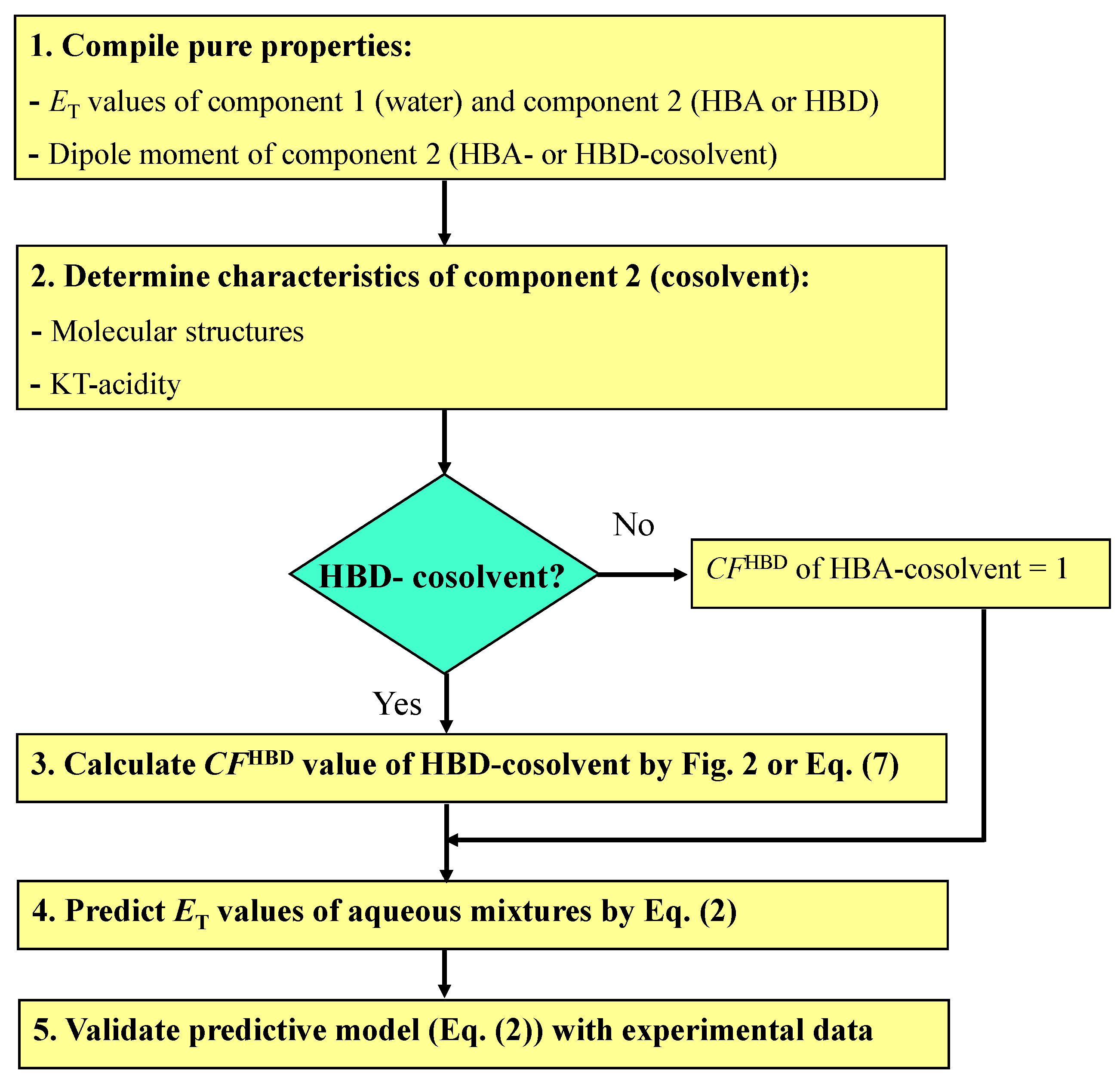
2.2. Predictive Model

A predictive model was originally proposed for estimating Kamlet–Taft dipolarity/polarizability (KT-π*) [22] of binary nonpolar-polar mixtures with an assumption that the gas-phase dipole moment (µ) of the polar component can quantify a trend of mixture KT-π* values at a fixed mole composition. Due to a linear relationship between KT-π* and E_T values (homomorphism line, Figure 2), the predictive model for KT-π* values can directly transform into a function form for estimating E_T values for nonpolar-polar mixtures reported in our previous work [20], as shown by Equation (2). In this work, the model (Equation (2)) was used to predict the E_T values of aqueous mixtures due to similar negative deviation trends in both aqueous mixtures and nonpolar-polar mixtures as mentioned in the introduction (Figure 1).

$$\Delta E_{\mathrm{T},\mathrm{m}\mathrm{i}x}^{\mathrm{N}}={\mu }_2\left(-x_1\ln (x_1+1.981x_2)-x_2\ln (x_2+0.181x_1)\right)\times C{F}^{\mathrm{HBD}}$$

(2)

where µ₂ is the gas-phase dipole moment of component 2. The 1.981 and 0.181 values are the universal Wilson constant parameters (Λ₁₂ and Λ₂₁) for predictions and were evaluated by correlating experimental data with Wilson thermodynamic excess function [22]. The $\Delta E_{\mathrm{T},\mathrm{m}\mathrm{i}x}^{\mathrm{N}}$ is relative normalized electronic transition energy and defined by Equations (3)–(5).

$$\Delta E_{\mathrm{T},\mathrm{m}\mathrm{i}x}^{\mathrm{N},}=E_{\mathrm{T},\mathrm{m}\mathrm{i}x}^{\mathrm{N}}-(x_1{E}_{\mathrm{T},1}^{\mathrm{N}}+x_2{E}_{\mathrm{T},2}^{\mathrm{N}})=E_{\mathrm{T},\mathrm{m}\mathrm{i}x}^{\mathrm{N}}-x_2$$

(3)

$$E_{\mathrm{T},\mathrm{m}\mathrm{i}x}^{\mathrm{N}}=\frac{E_{\mathrm{T},\mathrm{m}\mathrm{i}x}-E_{\mathrm{T},1}^0}{E_{\mathrm{T},2}^0-E_{\mathrm{T},1}^0}$$

(4)

$$E_{\mathrm{T}}(\mathrm{kcal}\cdot {\mathrm{mol}}^{-1})=28591/{\lambda }_{\max }(\mathrm{nm})$$

(5)

where λ_max (nm) is the maximum absorption of the wavelength of a solvatochromic indicator (Reichardt indicator) obtained from UV-Vis spectroscopy. The $E_{\mathrm{T},\mathrm{m}\mathrm{i}x}$ and $E_{\mathrm{T},\mathrm{m}\mathrm{i}x}^{\mathrm{N}}$ are the electronic transition energy and the normalized electronic transition energy of the binary mixtures. To apply the predictive model (Equation (2)) to aqueous systems studied in this work, component 1 refers to water and component 2 refers to cosolvent (HBA or HBD). According to normalization (Equation (4)), the $E_{\mathrm{T},1}^{\mathrm{N}}$ and $E_{\mathrm{T},2}^{\mathrm{N}}$ of pure components 1 and 2 in Equation (3) are set equal to zero and unity, respectively.

The CF^HBD parameter in Equation (2) is the HBD contribution factor and the parameter is only applied to an aqueous mixture of HBD cosolvents due to specific interaction of HBD solvent with indicator [20] that causes a deviation in the pure $E_{\mathrm{T},2}^0$ value (HBD solvent) from the homomorphism line (Figure 2). The CF^HBD values in Equation (6) can be estimated by a deviation of the actual E_T value of pure HBD cosolvent ($E_{\mathrm{T},2}^0$) from the homomorphism line in Figure 2 as shown in Equation (6).

$$C{F}^{\mathrm{HBD}}=E_T^{0,\mathrm{Non}}-E_{\mathrm{T},2}^0$$

(6)

where $E_T^{0,\mathrm{Non}}$ is a non-HBD bonding E_T value of pure HBD cosolvents defined as a linear function of dipolarity/polarizability (KT-π*), that is the homomorphism linear line in Figure 2. The linear relationships of $E_T^{0,\mathrm{Non}}$ were given in detail in our previous work [20], and the CF^HBD values of nine HBD cosolvents studied in this work are given in

Table 1. Pure properties of hydrogen bond donor (HBD) at 25 °C showing Kamlet–Taft acidity (KT-α) [27,28] and HBD contribution factor (CF^HBD) evaluated from three indicators (Ind.) ^a.

Entry	HBD Solvents	KT-α	Actual CFHBD (-) b				Calculated CFHBD (-) c
(Symbol)	(Abbreviation)	(-)	Ind. 1	Ind. 2	Ind. 3	Avg	(Equation (7))
1 ( )	Methanol (MeOH)	1.00	3.65	2.32	2.34	2.77	2.75
2 ( )	Ethanol (EtOH)	0.89	3.05	2.21	2.21	2.49	2.45
3 ( )	1-Propanol (PrOH)	0.84	2.79	1.96	2.51	2.42	2.31
4 ( )	2-Propanol (iPrOH)	0.76	2.44	1.72	2.17	2.11	2.09
5 ( )	1-Butanol (BuOH)	0.84	2.65	2.04	3.04	2.58	2.31
6 ( )	Tert-Butanol (T-BuOH)	-	2.65	-	-	2.65	-
7 ( )	Ethylene glycol (ETG)	0.90	3.01	-	1.59	2.30	2.48
8 ( )	Acetic acid (AcOH)	1.12	4.34	1.83	2.78	2.98	3.09
9 ( )	Formamide (FA)	0.63	2.09	1.27	1.32	1.56	1.73

^a Indicators: Ind. 1 = 2,6-diphenyl-4-(2,4,6-triphenyl-1-pyridinio) phenolate indicator; Ind. 2 = phenol blue and Ind. 3 = Nile red. ^b Actual CF^HBD values are evaluated from Figure 2. ^c Calculated CF^HBD values are obtained from Equation (7).

along with their Kamlet–Taft acidity (α).

An average CF^HBD value from three indicators (Table 1) was used in predictions (Equation (2)) for nine aqueous mixtures of HBD cosolvents. To extend to other HBD cosolvents, a linear relationship of CF^HBD with Kamlet–Taft acidity (α) was proposed in Equation (7) and Figure 3, because the α values of HBD cosolvents are widely available in the literature [27,28].

$$C{F}^{\mathrm{HBD}}=2.766\alpha -0.0115,({\mathrm{R}}^2=0.89)$$

(7)

Figure 4 shows a flow chart developed in this work for predicting E_T values of aqueous mixtures that is divided into five steps. In step 1, pure properties of electronic transition energy ($E_{\mathrm{T},\mathrm{i}}^0$) and gas-phase dipole moment (µ₂) of components 1 and 2 are compiled from the literature. In step 2, solvent characteristics of component 2 (cosolvent) are determined to check HBD ability by considering their molecular structures and KT-acidity. For example, HBD cosolvents are able to donate a proton so that their KT-acidity values are relatively high (Table 1). On the other hand, HBA cosolvents lack proton donor groups and, thus, the CF^HBD value of HBA cosolvent is equal to unity. In step 3, CF^HBD values of HBD cosolvent are calculated by either Figure 2 or Equation (7). In steps 4 and 5, the predictive model (Equation (2)) was used to estimate the E_T values of aqueous mixtures and was validated, respectively. To validate the predictive model in step 5, nine aqueous mixtures of HBA cosolvents and nine aqueous mixtures of HBD cosolvents (

Table 2. Comparison between electronic transition (E_T, kcal·mol⁻¹) values calculated with the predictive model (Equation (2)) and ideal model (Equation (1)) for nine aqueous mixtures of hydrogen bond acceptor (HBA) cosolvents and nine aqueous mixtures of hydrogen bond donor (HBD) cosolvents at 25 °C that were obtained with Reichardt indicator. Average relative deviations (ARD) were calculated with Equation (8) along with dipole moment of component 2 (µ₂), HBD contribution factor (CF^HBD), Hunter basicity (β^H) of component 2, pure properties of electronic transition energy ($E_{\mathrm{T},\mathrm{i}}^0$ ) and the number of data used (N). Gray-shaded rows indicate the ARD results estimated from the calculated CF^HBD (Equation (7)).

Entry	Component 2	µ2	CFHBD	βH	${\mathit{E}}_{\mathbf{T}}^0$		ARD (%)		N	Ref.
(Symbol)		D	(-)	(-)	(1)	(2)	Predict	Ideal
Water (1)—HBA cosolvent (2)
1 (■)	ACN	3.92	1.00	4.7	63.10	46.00	6.64	3.36	11	[15]
2 (■)	THF	1.63	1.00	5.3	63.10	37.50	4.36	4.97	11	[15]
3 (●)	GBL	3.82	1.00	5.3	63.00	44.62	3.45	4.42	12	[23]
4 (●)	GVL	5.30	1.00	5.3	63.00	47.85	2.61	6.27	12	[23]
5 (●)	PYR	3.10	1.00	8.3	63.00	47.90	1.49	5.24	11	[24]
6 (●)	NMP	4.09	1.00	8.3	63.00	42.20	1.85	9.85	10	[24]
7 (●)	DMF	3.86	1.00	8.3	63.10	43.80	1.37	4.77	11	[15]
8 (■)	DMSO	3.96	1.00	8.9	63.10	45.00	0.75	5.29	11	[15]
9 (■)	Pyridine	2.19	1.00	7.0	63.10	40.30	1.29	4.77	11	[15]
		Overall (aqueous HBA mixtures)						2.65	5.44
Water (1)—HBD cosolvent (2)
10 ( )	MeOH	1.70	2.77	5.8	63.10	55.70	0.23	2.40	11	[15]
			2.75				0.23
11 ( )	EtOH	1.69	2.49	5.8	63.10	51.70	0.34	3.92	11	[15]
			2.45				0.38
12 ( )	PrOH	1.66	2.42	5.8	63.10	50.60	1.42	5.14	11	[15]
			2.31				1.53
13 ( )	iPrOH	1.66	2.11	5.8	63.10	48.70	2.64	6.73	11	[15]
			2.09				2.67
14 ( )	BuOH	1.66	2.58	5.8	63.10	43.90	2.58	4.28	10	[15]
			2.31				2.19
15 ( )	T-BuOH	1.67	2.65	5.8	63.10	43.30	4.67	12.54	11	[25]
16 ( )	ETG	2.31	2.30	-	63.10	56.24	0.50	2.44	10	[15]
			2.48				0.69
17 ( )	AcOH	1.74	2.98	5.3	63.10	55.00	1.03	2.10	11	[15]
			3.09				1.12
18 ( )	FA	3.73	1.56	5.8	63.10	53.74	0.97	3.22	11	[15]
			1.73				1.32
		Overall (aqueous HBD mixtures)						1.60	4.75
	Overall (both HBA and HBD mixtures)							2.12	5.10	197

The µ₂ values for all solvents are taken from handbook [29], except for GVL [32]. The overall average relative deviation (ARD) values are calculated without considering the values in the gray-shaded rows. Solvent abbreviations for HBD cosolvent are given in Table 1. Solvent abbreviations for HBA cosolvent: ACN = acetonitrile; THF = tetrahydrofuran; GBL = gamma butyrolactone; GVL = gamma valerolactone; PYR = 2-pyrrolidinone; NMP = N-methyl-2-pyrrolidone; DMF = dimethylformamide and DMSO = dimethyl sulfoxide.

) were used and discussed in Section 3. Table 2 tabulates the $E_{\mathrm{T},\mathrm{i}}^0$, µ₂ [29], Hunter basicity (β^H) of component 2 [30,31] and CF^HBD values of solvents used in the predictions.

2.3. Evaluation of the Frameworks

Average relative deviation (ARD) was used to evaluate a deviation between experimental ($E_{\mathrm{T}}^{\mathrm{Exp}}$) and calculated ($E_{\mathrm{T}}^{\mathrm{Cal}}$) data as shown in Equation (8):

$$\mathrm{ARD}(\%)=(1/N){\displaystyle \sum \left|(E_{\mathrm{T}}^{\mathrm{Cal}}-E_{\mathrm{T}}^{\mathrm{Exp}})/E_{\mathrm{T}}^{\mathrm{Exp}}\right|}\times 100$$

(8)

3. Results and Discussion

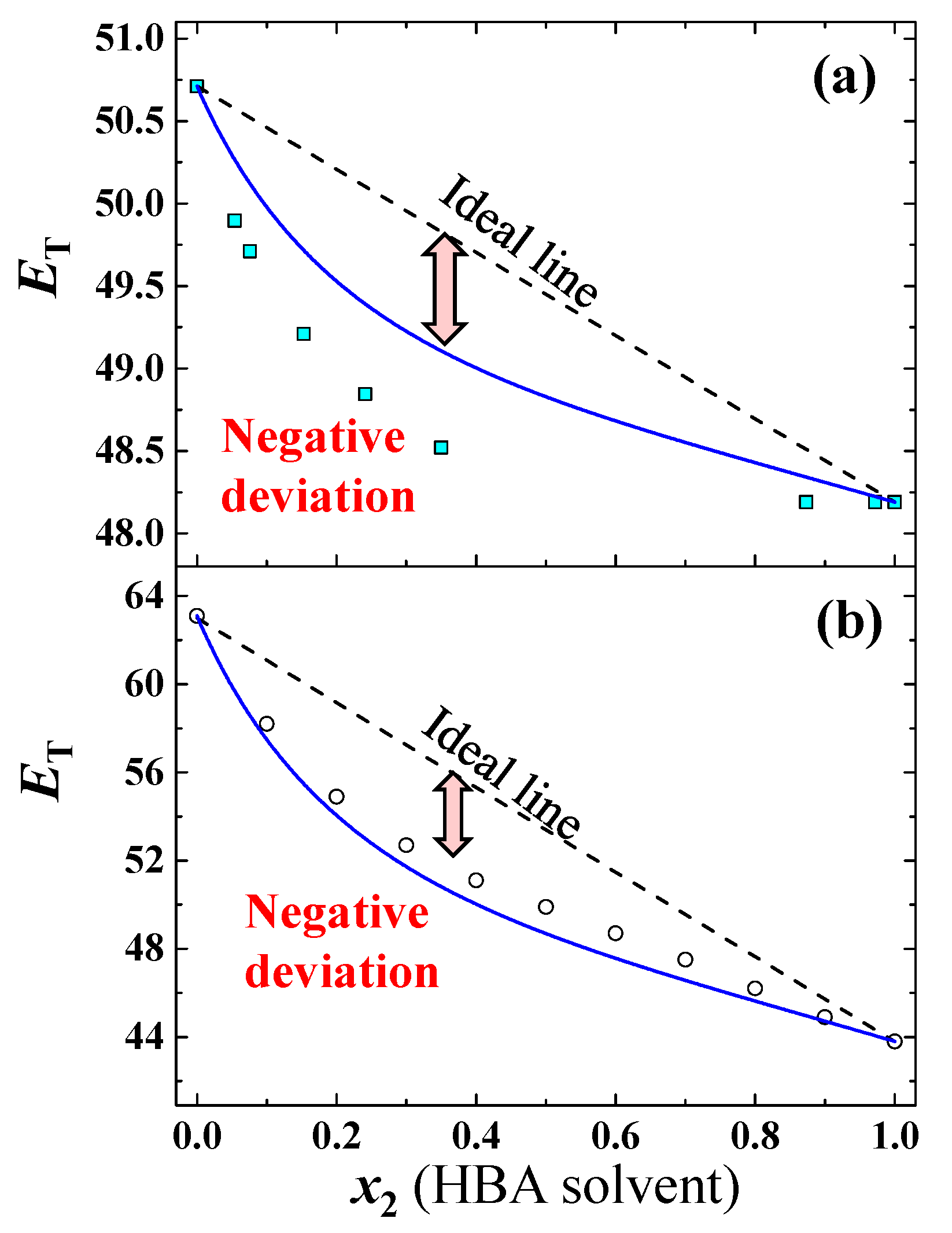
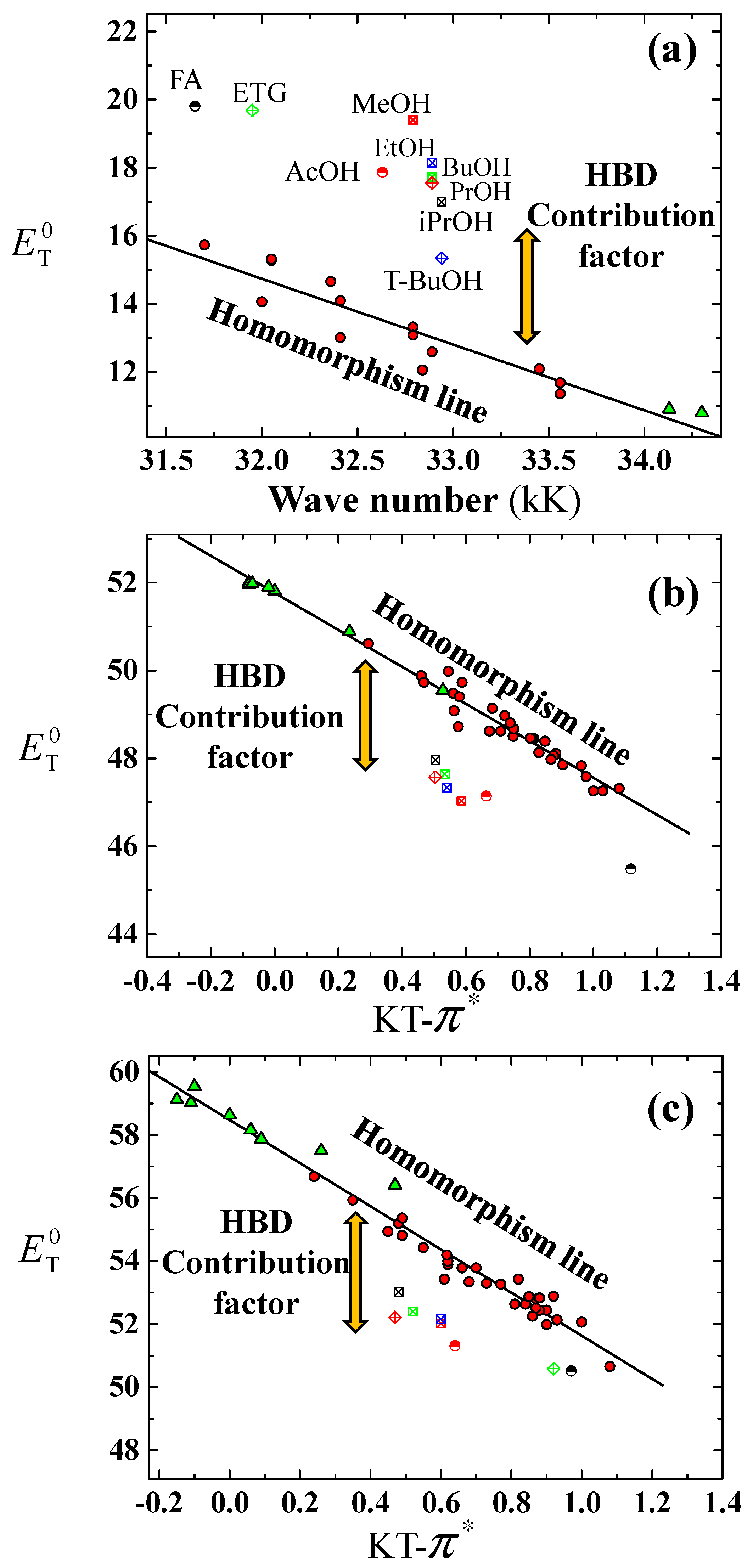
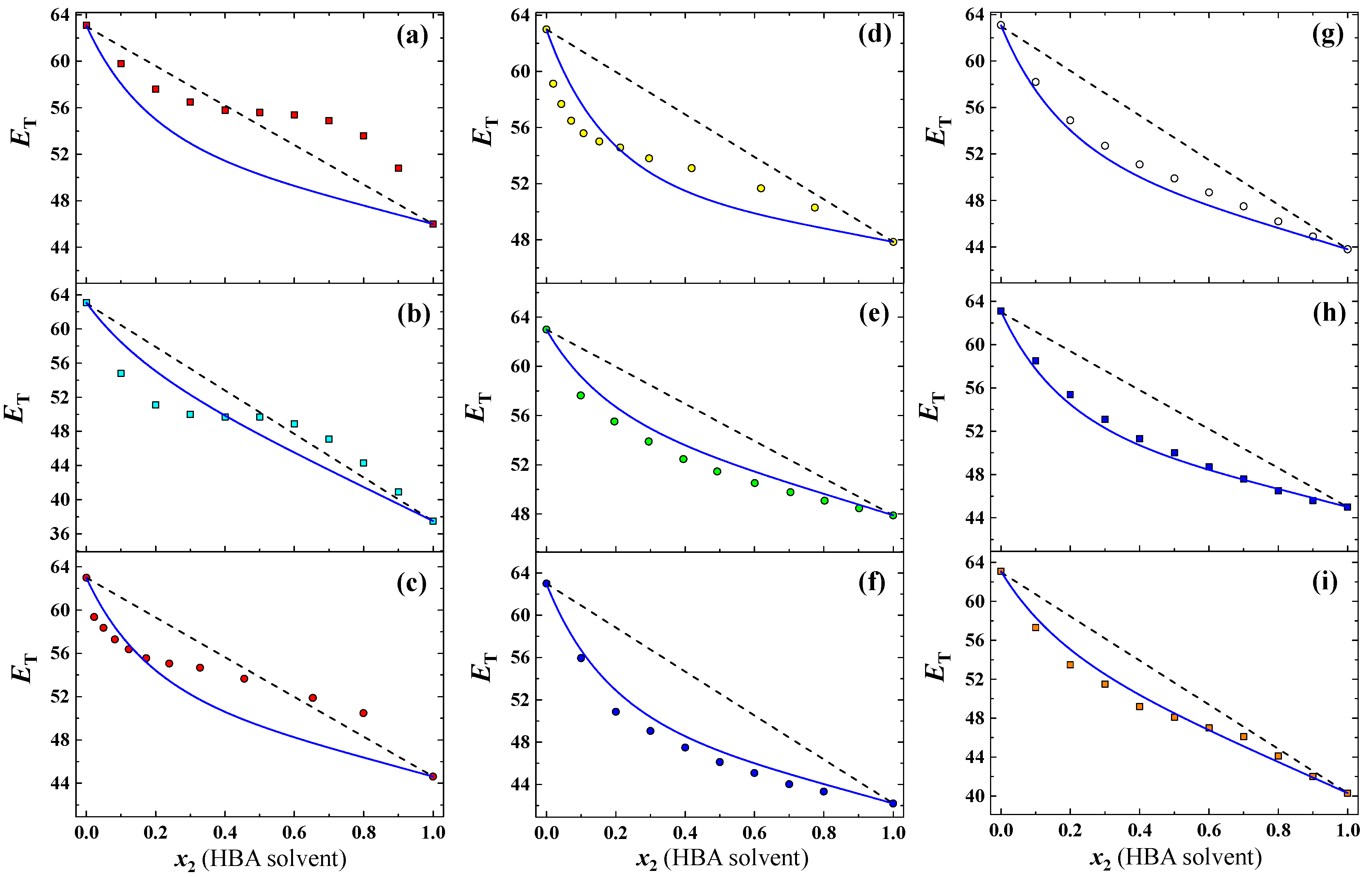
3.1. Prediction for Aqueous Mixtures of HBA Cosolvents

Figure 5 shows the E_T values of nine aqueous mixtures of water (1)—HBA cosolvent (2) as a function of component 2 (HBA cosolvent). The E_T values of all aqueous mixtures (Figure 5) exhibited a negative deviation from the ideality (dashed lines, Figure 5), except for the aqueous mixtures of acetonitrile (ACN), tetrahydrofuran (THF) and gamma-butyrolactone (GBL) that showed a sigmoid function (Figure 5a–c). Blue solid lines (Figure 5) show predicted E_T values of the aqueous mixture using Equation (2) without CF^HBD value (CF^HBD = 1) that generally tended toward the experimental data (symbols, Figure 5).

Table 2 shows a comparison of ARD values obtained between the ideal model (Equation (1)) and predictive model (Equation (2)) for the aqueous mixtures of HBA cosolvents (entries 1–9, Table 2) and HBD cosolvent (entries 10–18, Table 2). The predictive model (Equation (2)) generally provided a lower ARD value (2.7%, entries 1–9, Table 2) than that estimated from the ideal model (5.4%). However, the model gave a relatively high ARD value (entries 1–3, Table 2) for the aqueous mixtures that showed the sigmoid functions (Figure 5a–c). These results inferred a limitation of the predictive model and were discussed later in Section 3.4. The predictive results of aqueous mixtures of HBD cosolvents were discussed in the following section.

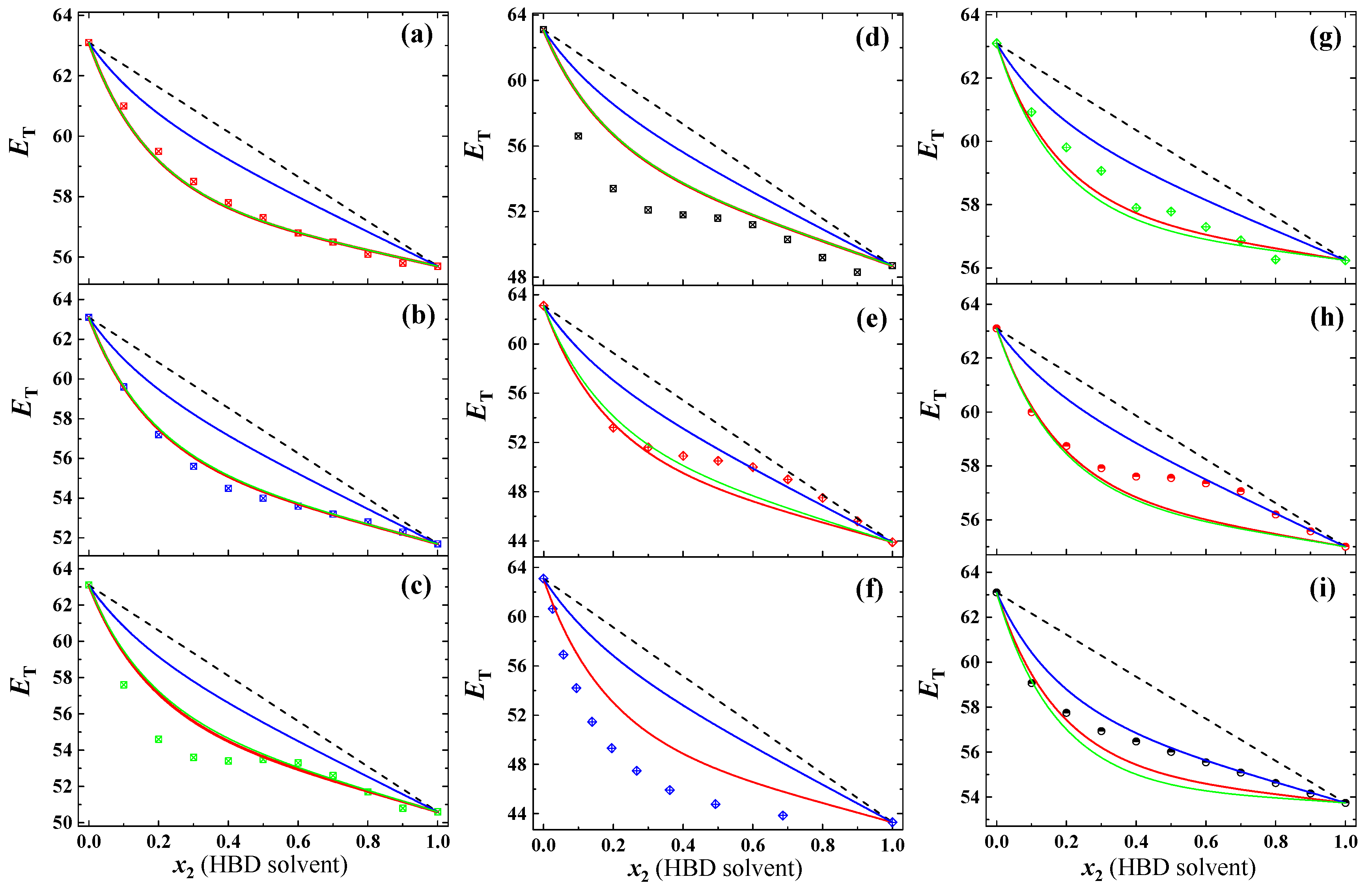
3.2. Prediction for Aqueous Mixtures of HBD Cosolvents

Figure 6 shows the E_T values of nine aqueous mixtures of water (1)—HBD solvent (2) as a function of component 2 (HBD solvent) that also exhibited a negative deviation from the ideality. A comparison in predictive model (Equation (2)) with considering CF^HBD value (Table 1) and without considering CF^HBD value (CF^HBD = 1). Red solid lines in Figure 6 show predictions with considering CF^HBD value, while the blue ones are the predictions without considering CF^HBD value.

The predictive model with the addition of CF^HBD values (red solid lines, Figure 6) could provide a better result in the calculated E_T value that followed the experimental data than the result without the CF^HBD value (blue solid lines, Figure 6). The ARD values obtained from the predictive model (Equation (2)) with considering CF^HBD value (1.6%, entries 10–18, Table 2) are lower than those estimated from the ideal model (4.8%). Figure 7 shows parity plots of calculated E_T values that are estimated from the predictive model (Figure 7a) and the ideal model (Figure 7b). The estimated E_T values from the predictive model (R² = 0.91, Figure 7a) are less scattered than those obtained from the ideal model (R² = 0.81, Figure 7b).

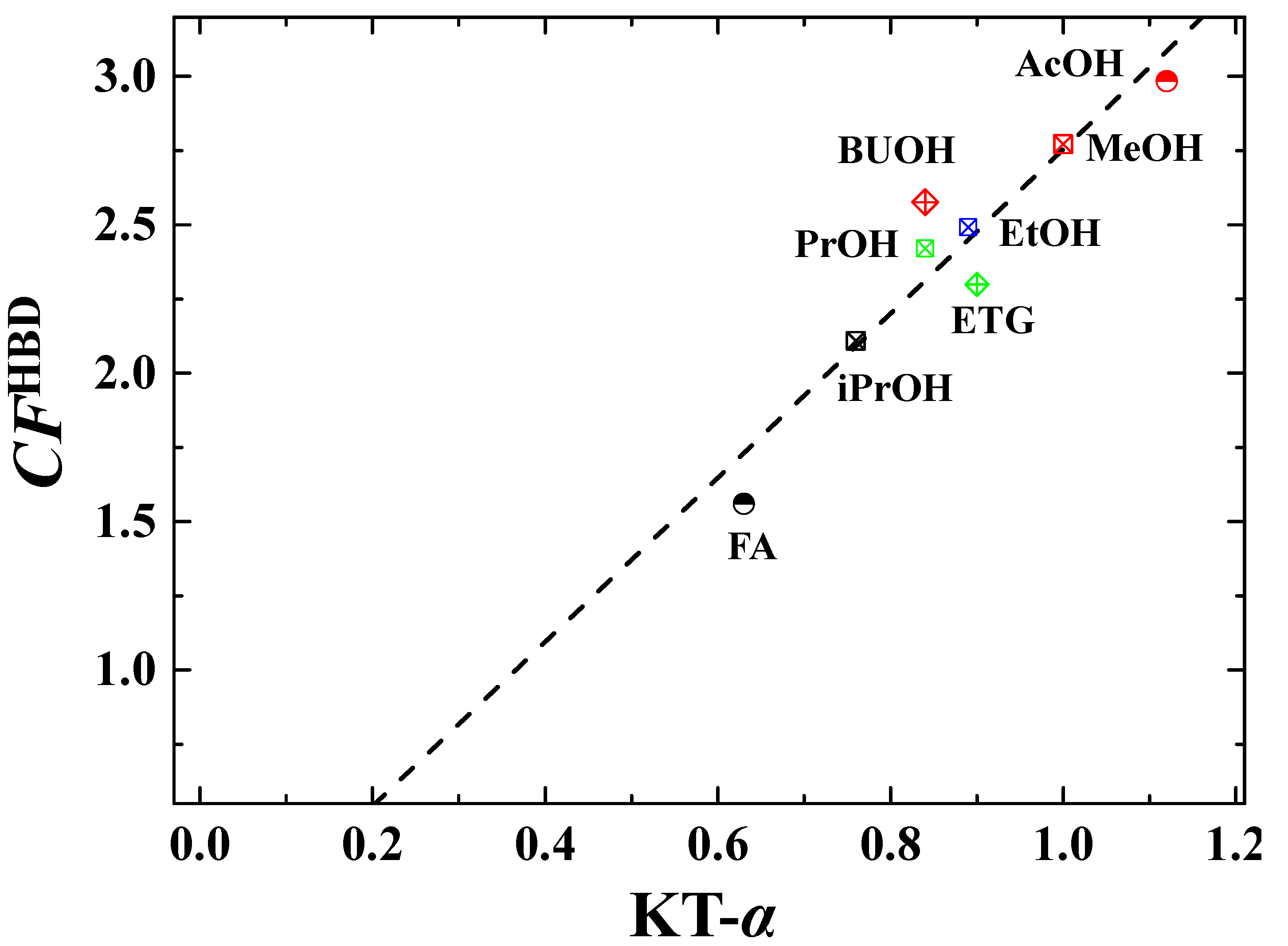
3.3. Evaluation of CF^HBD Methods for Predictions

In Section 3.2, the predicted E_T values of aqueous mixtures of HBD cosolvents were estimated based on the actual CF^HBD values evaluated from Figure 2 and Table 1. In the section, a comparison in evaluated E_T values between actual data (Table 1) and calculations with KT-acidity (Equation (7)) was made for predictions. Red solid lines (Figure 6) show predicted E_T values of the mixtures with actual CF^HBD values, while the green solid lines (Figure 6) show predictions using calculated CF^HBD values from the correlation (Equation (7)). The predictive model with the calculated CF^HBD values provided a similar trend in predictions with the actual CF^HBD values (Figure 6), in which the ARD values from the calculated CF^HBD (gray-shaded rows, Table 2) are comparable to those estimated from the actual ones (entries 10–18, Table 2).

3.4. Limitation of the Predictive Model

According to predictive results in Section 3.1, the model (Equation (2)) provided a high ARD value for aqueous mixtures having a sigmoid function (entries 1–3, Table 2). Marcus reported [33,34] that the sigmoid trends were found in aqueous mixtures when microheterogeneity occurred. It is expected that the microheterogeneity phenomenon caused a high error in predictions because this phenomenon was not considered in the development of the model as mentioned in Section 2.2. Hunter basicity of HBA solvents (β^H, Table 2) can quantify the hydration shell strength in aqueous mixtures [35]. It was found that the sigmoid behaviors occurred in the aqueous mixtures that have low β^H values (β^H ≤ 5.3, entries 1–3, Table 2). Thus, the model (Equation (2)) is effective for predicting the aqueous mixtures having high β^H values (β^H ≥ 5.3).

4. Conclusions

In this work, a predictive model is proposed for estimating the solvatochromic polarity of electronic transition energy (E_T) for aqueous mixtures. The function form for E_T values for aqueous mixtures can be adopted from the previous model for nonpolar-polar mixtures due to similar interactions and trends in the mixture E_T values in both systems. The predictive model was validated by eighteen aqueous mixtures and was found to give a reliable E_T value with an overall deviation of 2.1%. Three properties of pure components are basically needed for predictions: (i) E_T values, (ii) gas-phase dipole moment and (iii) Kamlet–Taft acidity.

References

1. Guo, H.; Duereh, A.; Su, Y.; Hensen, E.J.M.; Qi, X.; Smith, R.L. Mechanistic role of protonated polar additives in ethanol for selective transformation of biomass-related compounds. Appl. Catal. B 2020, 264, 118509. [Google Scholar] [CrossRef]
2. Ghatta, A.A.; Wilton-Ely, J.D.E.T.; Hallett, J.P. Rapid, High-Yield Fructose Dehydration to 5-Hydroxymethylfurfural in Mixtures of Water and the Noncoordinating Ionic Liquid [bmim][OTf]. ChemSusChem 2019, 12, 4452–4460. [Google Scholar] [CrossRef]
3. Pingali, S.V.; Smith, M.D.; Liu, S.H.; Rawal, T.B.; Pu, Y.; Shah, R.; Evans, B.R.; Urban, V.S.; Davison, B.H.; Cai, C.M.; et al. Deconstruction of biomass enabled by local demixing of cosolvents at cellulose and lignin surfaces. Proc. Natl. Acad. Sci. USA 2020, 107, 16776–16781. [Google Scholar] [CrossRef]
4. Farajtabar, A.; Zhao, H. Equilibrium solubility of 7-amino-4-methylcoumarin in several aqueous co-solvent mixtures revisited: Transfer property, solute-solvent and solvent-solvent interactions and preferential solvation. J. Mol. Liq. 2020, 320, 114407. [Google Scholar] [CrossRef]
5. Zheng, M.; Farajtabar, A.; Zhao, H. Solubility of 4-amino-2,6-dimethoxypyrimidine in aqueous co-solvent mixtures revisited: Solvent effect, transfer property and preferential solvation analysis. J. Mol. Liq. 2019, 288, 111033. [Google Scholar] [CrossRef]
6. Zhu, C.; Farajtabar, A.; Wu, J.; Zhao, H. 5,7-Dibromo-8-hydroxyquinoline dissolved in binary aqueous co-solvent mixtures of isopropanol, N,N-dimethylformamide, 1,4-dioxane and N-methyl-2-pyrrolidone: Solubility modeling, solvent effect and preferential solvation. J. Chem. Thermodyn. 2020, 148, 106138. [Google Scholar] [CrossRef]
7. Piccione, P.M.; Baumeister, J.; Salvesen, T.; Grosjean, C.; Flores, Y.; Groelly, E.; Murudi, V.; Shyadligeri, A.; Lobanova, O.; Lothschütz, C. Solvent Selection Methods and Tool. Org. Process Res. Dev. 2019, 23, 998–1016. [Google Scholar] [CrossRef]
8. Byrne, F.P.; Forier, B.; Bossaert, G.; Hoebers, C.; Farmer, T.J.; Hunt, A.J. A methodical selection process for the development of ketones and esters as bio-based replacements for traditional hydrocarbon solvents. Green Chem. 2018, 20, 4003–4011. [Google Scholar] [CrossRef] [Green Version]
9. Jin, S.; Byrne, F.; McElroy, C.R.; Sherwood, J.; Clark, J.H.; Hunt, A.J. Challenges in the development of bio-based solvents: A case study on methyl(2,2-dimethyl-1,3-dioxolan-4-yl)methyl carbonate as an alternative aprotic solvent. Faraday Discuss. 2017, 202, 157–173. [Google Scholar] [CrossRef] [Green Version]
10. Duereh, A.; Sato, Y.; Smith, R.L.; Inomata, H. Methodology for Replacing Dipolar Aprotic Solvents Used in API Processing with Safe Hydrogen-Bond Donor and Acceptor Solvent-Pair Mixtures. Org. Process Res. Dev. 2017, 21, 114–124. [Google Scholar] [CrossRef] [Green Version]
11. Song, B.; Yu, Y.; Wu, H. Solvent effect of gamma-valerolactone (GVL) on cellulose and biomass hydrolysis in hot-compressed GVL/water mixtures. Fuel 2018, 232, 317–322. [Google Scholar] [CrossRef]
12. Katritzky, A.R.; Fara, D.C.; Yang, H.; Tämm, K.; Tamm, T.; Karelson, M. Quantitative Measures of Solvent Polarity. Chem. Rev. 2004, 104, 175–198. [Google Scholar] [CrossRef] [PubMed]
13. Pires, P.A.R.; El Seoud, O.A.; Machado, V.G.; de Jesus, J.C.; de Melo, C.E.A.; Buske, J.L.O.; Cardozo, A.P. Understanding Solvation: Comparison of Reichardt’s Solvatochromic Probe and Related Molecular “Core” Structures. J. Chem. Eng. Data 2019, 64, 2213–2220. [Google Scholar] [CrossRef]
14. Reichardt, C. Solvatochromic Dyes as Solvent Polarity Indicators. Chem. Rev. 1994, 94, 2319–2358. [Google Scholar] [CrossRef]
15. Marcus, Y. The use of chemical probes for the characterization of solvent mixtures. Part 2. Aqueous mixtures. J. Chem. Soc. Perkin Trans. 1994, 2, 1751–1758. [Google Scholar] [CrossRef]
16. Roses, M.; Buhvestov, U.; Rafols, C.; Rived, F.; Bosch, E. Solute-solvent and solvent-solvent interactions in binary solvent mixtures. Part 6. A quantitative measurement of the enhancement of the water structure in 2-methylpropan-2-ol-water and propan-2-ol-water mixtures by solvatochromic indicators. J. Chem. Soc. Perkin Trans. 1997, 2, 1341–1348. [Google Scholar] [CrossRef]
17. Duereh, A.; Sato, Y.; Smith, R.L.; Inomata, H. Correspondence between spectral-derived and viscosity-derived local composition in binary liquid mixtures having specific interactions with preferential solvation theory. JPC B 2018, 122, 10894–10906. [Google Scholar] [CrossRef]
18. Duereh, A.; Guo, H.; Honma, T.; Hiraga, Y.; Sato, Y.; Lee Smith, R.; Inomata, H. Solvent polarity of cyclic ketone (cyclopentanone, cyclohexanone): Alcohol (methanol, ethanol) renewable mixed-solvent systems for applications in pharmaceutical and chemical processing. Ind. Eng. Chem. Res. 2018, 57, 7331–7344. [Google Scholar] [CrossRef]
19. Jouyban, A.A.G.; Khoub Nasab Jafari, M.; Eugen Acree, W., Jr. Modeling the solvatochromic parameter (e) of mixed solvents with respect to solvent composition and temperature using the jouyban-acree model. Daru J. Pharm. Sci. 2006, 14, 22–25. [Google Scholar]
20. Duereh, A.; Inomata, H. Prediction of solvatochromic parameters of electronic transition energy for characterizing dipolarity/polarizability and hydrogen bonding donor interactions in binary solvent systems of liquid nonpolar-polar mixtures, CO2-expanded liquids and supercritical carbon dioxide with cosolvent. J. Mol. Liq. 2020, 320, 114394. [Google Scholar]
21. Duereh, A.; Sugimoto, Y.; Ota, M.; Sato, Y.; Inomata, H. Kamlet–Taft dipolarity/polarizability of binary mixtures of supercritical carbon dioxide with cosolvents: Measurement, prediction, and applications in separation processes. Ind. Eng. Chem. Res. 2020, 59, 12319–12330. [Google Scholar] [CrossRef]
22. Duereh, A.; Guo, H.; Sato, Y.; Smith, R.L.; Inomata, H. Predictive framework for estimating dipolarity/polarizability of binary nonpolar–polar mixtures with relative normalized absorption wavelength and gas-phase dipole moment. Ind. Eng. Chem. Res. 2019, 58, 18986–18996. [Google Scholar] [CrossRef]
23. Duereh, A.; Sato, Y.; Smith, R.L.; Inomata, H. Analysis of the Cybotactic Region of Two Renewable Lactone–Water Mixed-Solvent Systems that Exhibit Synergistic Kamlet–Taft Basicity. JPC B 2016, 120, 4467–4481. [Google Scholar] [CrossRef]
24. García, B.; Aparicio, S.; Alcalde, R.; Ruiz, R.; Dávila, M.J.; Leal, J.M. Characterization of Lactam-Containing Binary Solvents by Solvatochromic Indicators. JPC B 2004, 108, 3024–3029. [Google Scholar] [CrossRef]
25. Sindreu, R.; Moyá, M.; Sánchez Burgos, F.; González, A.G. Kamlet-Taft solvatochromic parameters of aqueous binary mixtures oftert-butyl alcohol and ethyleneglycol. J. Solut. Chem. 1996, 25, 289–293. [Google Scholar] [CrossRef]
26. Mellein, B.R.; Aki, S.N.V.K.; Ladewski, R.L.; Brennecke, J.F. Solvatochromic studies of ionic liquid/organic mixtures. JPC B 2007, 111, 131–138. [Google Scholar] [CrossRef] [PubMed]
27. Taft, R.W.; Kamlet, M.J. The solvatochromic comparison method. 2. The alpha-scale of solvent hydrogen-bond donor (HBD) acidities. J. Am. Chem. Soc. 1976, 98, 2886–2894. [Google Scholar] [CrossRef]
28. Kamlet, M.J.; Abboud, J.L.M.; Abraham, M.H.; Taft, R.W. Linear solvation energy relationships. 23. A comprehensive collection of the solvatochromic parameters, .pi.*, .alpha., and .beta., and some methods for simplifying the generalized solvatochromic equation. J. Org. Chem. 1983, 48, 2877–2887. [Google Scholar] [CrossRef]
29. Yaws, C. Chemical Properties Handbook: Physical, Thermodynamics, Environmental Transport, Safety and Health Related Properties for Organic and Inorganic Chemicals; McGraw-Hill Education: New York, NY, USA, 1999. [Google Scholar]
30. Hunter, C.A. Quantifying intermolecular interactions: Guidelines for the molecular recognition toolbox. Angew. Chem. 2004, 43, 5310–5324. [Google Scholar] [CrossRef] [PubMed]
31. Duereh, A.; Smith, R.L. Strategies for using hydrogen-bond donor/acceptor solvent pairs in developing green chemical processes with supercritical fluids. J. Supercrit. Fluids 2018, 141, 182–197. [Google Scholar] [CrossRef]
32. He, J.; Liu, M.; Huang, K.; Walker, T.W.; Maravelias, C.T.; Dumesic, J.A.; Huber, G.W. Production of levoglucosenone and 5-hydroxymethylfurfural from cellulose in polar aprotic solvent-water mixtures. Green Chem. 2017, 19, 3642–3653. [Google Scholar] [CrossRef]
33. Migron, Y.; Marcus, Y. Polarity and hydrogen-bonding ability of some binary aqueous-organic mixtures. J. Chem. Soc. Faraday Trans. 1991, 87, 1339–1343. [Google Scholar] [CrossRef]
34. Marcus, Y.; Migron, Y. Polarity, hydrogen bonding, and structure of mixtures of water and cyanomethane. JPC 1991, 95, 400–406. [Google Scholar] [CrossRef]
35. Duereh, A.; Sato, Y.; Smith, R.L.; Inomata, H.; Pichierri, F. Does Synergism in Microscopic Polarity Correlate with Extrema in Macroscopic Properties for Aqueous Mixtures of Dipolar Aprotic Solvents? JPC B 2017, 121, 6033–6041. [Google Scholar] [CrossRef] [PubMed]
Figure 1. Comparison in electronic transition (ET, kcal·mol−1) for (a) nonpolar-polar systems of carbon tetrachloride (1)—dimethylformamide (2) and (b) aqueous systems of water (1)—dimethylformamide (2) as a function of mole composition of component 2 (x2) at 25 °C. Black dashed lines show calculations from the ideal model (Equation (1)). Blue solid lines show predictions with the predictive model (Equation (2)) without considering hydrogen bond donor (HBD) contribution factor (CFHBD = 1). The ET values in part (a) were collected from the phenol blue indicator [26]. The ET values in part (b) were obtained from the Reichardt indicator [15].
Applsci 10 08480 g001
Figure 2. Plot of Kamlet–Taft dipolarity/polarizability (KT-π*) and electronic transition ( E T 0 , kcal·mol−1) of three indicators as (a) Reichardt indicator, (b) phenol blue indicator and (c) Nile red indicator in () pure nonpolar solvent, () pure hydrogen bond acceptor (HBA) solvent and pure polar hydrogen bond donor (HBD) solvent. Symbols of HBD solvents are given in Table 1. Solid line shows a linear relationship (reference homomorphism line) of KT-π* values and ET values of pure nonpolar solvents and pure HBA solvents. The deviation of ET values of pure HBD solvents from the linear line is due to HBD contribution. Data are given in detail in our previous work [20].
Applsci 10 08480 g002
Figure 3. Relationship of HBD contribution factor (CFHBD) with Kamlet–Taft acidity (KT-α) of hydrogen bond donor (HBD) cosolvents at 25 °C. The CFHBD and KT-α data are given in Table 1. Dashed line represents Equation (7). Symbols of HBD solvents are given in Table 1.
Applsci 10 08480 g003
Figure 4. Flow chart for predicting electronic transition (ET) of aqueous mixture with five steps.
Applsci 10 08480 g004
Figure 5. Electronic transition of (ET (30), kcal·mol−1) of nine aqueous mixtures of water (1)—hydrogen bond acceptor (HBA, 2) as a function of mole composition of component 2 (x2) at 25 °C. Symbols (ai) and reference sources are given in Table 2 (entries 1–9). Black dashed lines show calculations from the ideal model (Equation (1)). Blue solid lines show predictions with the predictive model (Equation (2)) without considering HBD contribution factor (CFHBD = 1).
Applsci 10 08480 g005
Figure 6. Electronic transition of (ET (30), kcal·mol−1) of nine aqueous mixtures of water (1)—hydrogen bond donor (HBD, 2) as a function of mole composition of component 2 (x2) at 25 °C. Symbols (ai) and reference sources are given in Table 2 (entries 10–18). Black dashed lines show calculations from the ideal model (Equation (1)). Blue solid lines show predictions with the predictive model (Equation (2)) without considering HBD contribution factor (CFHBD = 1). Red solid lines show prediction with the predictive model (Equation (2)) with considering actual CFHBD values in Table 1. Green solid lines show prediction with the predictive model (Equation (2)) with considering calculated CFHBD values using Equation (7).
Applsci 10 08480 g006
Figure 7. Parity plots of electronic transition (ET) in eighteen aqueous mixtures obtained from (a) the predictive model (Equation (2), R2 = 0.91) and (b) the ideal model (Equation (1), R2 = 0.81). Symbols and conditions are defined in Table 2.
Applsci 10 08480 g007