Abstract
Prognostic techniques play a critical role in predicting upcoming faults and failures in machinery or a system by monitoring any deviation in the operation. This paper presents a novel method to analyze multidimensional sensory data and use its characteristics in bearing health prognostics. Firstly, detrended fluctuation analysis (DFA) is exploited to evaluate the long-range correlations in ball bearing vibration data. The results reveal the existence of the crossover phenomenon in vibration data with two scaling exponents at the short-range and long-range scales. Among several data sets, applying the DFA method to vibration signals shows a consistent increase in the short-range scaling exponent toward bearing failure. Finally, Kendall’s tau is used as a ranking coefficient to quantify the trend in the scaling exponent. It was found that the Kendall’s tau coefficient of the vibration scaling exponent could provide an early warning signal (EWS) for bearing failure.
1. Introduction
Rolling element bearings (REBs) are one of the essential elements in rotary machinery, such as pumps, compressors, gearboxes, and electric motors. Usually, REBs are susceptible to catastrophic failures when they are operating under abnormal conditions, including heavier loading, corrosion, overheating, etc. As a result of frequent wear and friction, they will experience a gradual degradation and functionality loss during their operation. Evidently, REBs go through different stages (mild, moderate, and serious) of functionality loss before their failure.
Prognostics and diagnostics have been active research areas in recent years [1,2]. Diagnostic techniques evaluate the fault severity during operation to help in planning immediate reactive maintenance and avoiding any future failure. Usually, once a bearing fault has been detected, the time remaining before bearing failure is relatively very short. So, reactive maintenance often cannot be completed before the failure. On the other hand, prognostic techniques provide an early warning for bearing breakdown to plan the needed maintenance ahead of time. That permits a continuous and reliable operation of the mechanical system while enabling proactive maintenance.
The prognostic techniques can be classified into three categories: physics-based models (PbMs), data-driven model (DDMs), and hybrid models. The PbM approach depends on the mechanical component models to determine its deterioration over time. Moreover, the hybrid model approach is a combination of the PbM and DDM approaches. The main challenge in these two approaches is the difficulty of deriving the mathematical models accurately. On the other hand, the DDM approach extracts the features in the data collected from the mechanical component to determine its proximity to a failure. It is considered a trusted approach in predicting future failures. In general, the DDM approach has two subcategories: the machine-learning approach [3,4,5] and the statistical-based approach.
The statistical-based approach is based on several techniques in the time and frequency domains. In the time domain, the root mean square (RMS) is used to detect the starting point of bearing fault from its vibration data [6]. Furthermore, advanced statistical features, such as kurtosis [7], are applied to predict the remaining useful life (RUL) of bearings. On the other hand, novel frequency-domain statistical parameters, such as envelope spectrum and spectral kurtosis (SK) [8,9], are proposed to detect bearing fault features.
Medjaher et al. have studied the correlation between nominal and degraded vibration signals to estimate the RUL of bearings [10]. Li et al. have used an improved exponential model and a particle filter (PF) to predict bearing failure [11]. The adoption of one statistical model does not explain the discrepancy between the different degradation rates in the vibration data. Wang et al. have developed a multi-mode PF to track the different stages of bearing performance degradation [12]. Ahmad et al. have proposed adaptive predictive models to understand the trend in the vibration data and predict bearing failure [13]. Singleton et al. have estimated the extended Kalman filter parameters to predict bearing failure under different operating conditions [14]. Soualhi et al. have used Hilbert–Huang transform to monitor ball bearings and track their degradation [15].
The statistical techniques have different approaches to predict bearing failure up to a certain level. However, the used statistical features in these approaches have no clear trend of degradation or monotonic change over time before bearing failure. Moreover, despite signal denoising, the statistical parameters keep fluctuating over time and sometimes go through a sudden spike when bearings near their end of life. From the prognostics point of view, these drawbacks limit the usage of these statistical methods in practical applications. In this paper, using detrended fluctuation analysis (DFA), we propose a new health indicator (scaling exponent) to anticipate bearing degradation.
DFA has been used extensively in diagnostic techniques to identify and classify faults. As vibration signals are known to be non-stationary, DFA is one of the reliable methods to study the long-range correlations in these signals. Hu et al. have used DFA and variational model decomposition (VMD) to diagnose and classify the acquired vibration signals at different fault severities [16]. Wang et al. have applied DFA to gear vibrational signals for fault diagnostic purposes and concluded that DFA is capable of identifying gear faults to a reasonable extent [17]. Lin et al. have applied DFA to roller bearing fault data to diagnose the faults and showed that DFA delivers excellent extraction of features of non-stationary and nonlinear data [18].
The main contributions of this paper can be summarized in three main points. Firstly, the DFA method combined with Kendall’s tau introduce a novel health indictor of bearing degradation. The proposed indicator is corroborated using vibration signals collected from 17 bearings under different operating conditions. Secondly, the novel combined approach shows evidence of critical slowing down in the bearing vibration signals. The existence of the critical slowing down could provide a universal EWS for the failure of bearings and other components in rotary machinery. Finally, most of the classical health indicators used in the prognostics have shown a fluctuating trend toward bearing failure; however, the proposed method reveals a persistent trend in the scaling exponent of the vibration signals at an early stage of bearing degradation.
The rest of the paper is organized as follows. Section 2 provides a description of the testing platform and the vibration data sets. In Section 3, the DFA method and the Kendall’s tau coefficient are explained. Section 4 summarizes the results and the proposed approach. Finally, Section 5 presents the conclusions of the paper.
2. Experimental Platform and Vibration Data Sets
2.1. Experimental Configuration
The experimental platform PRONOSTIA is a test bed used in the IEEE PHM 2012 prognostic challenge to collect real data from ball bearings under accelerated degradation tests [19]. These tests provide real experimental data sets that characterize the degradation of the complete operational life in only a few hours. Under different operating conditions, vibration data are collected from several ball bearings before their failure. In the experiment, the ball bearings (NSK 6804DD) are examined throughout the different tests. As shown in Figure 1, the experimental platform PRONOSTIA consists of three main parts: a rotating module, a loading module, and a measurement module. The three modules are summarized below:
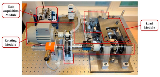
Figure 1.
Main modules of the experimental platform.
- The rotating module: it is composed of an asynchronous motor, a primary shaft, a speed reducer (gearbox), and a secondary shaft with a speed sensor. The asynchronous motor has a rated power of 250 W and an output speed of 2830 rpm. The gearbox consists of two pulleys connected by a timing belt. The main function of the gearbox is maintaining the speed of the secondary shaft at less than 2000 rpm while delivering a rated torque.
- The loading module: this has a pneumatic jack that generates a force acting on a lever arm. Then, the lever arm amplifies this force and transmits it as a radial force to the ball bearing under test. Adjusting the lever arm can help create different loading conditions on the bearing.
- The measurement module: different types of sensors are used to measure the radial force applied on the bearing, the rotation speed of the secondary shaft holding the bearing, and the torque delivered to the bearing. In addition, two high-frequency accelerometers (DYTRAN 3035B) are mounted perpendicularly to measure the horizontal and the vertical accelerations during the degradation test. In the measurement system, the temperature of the tested bearing is measured via one temperature sensor (PT100).
The main components in the experimental platform are shown in Figure 2. In the experiment, the ball bearings (NSK 6804DD) are deep groove, radial, and double rubber sealed. As shown in Figure 2, the dimensions of the bearings are . In addition, all the technical data of the ball bearing are shown in Table 1.
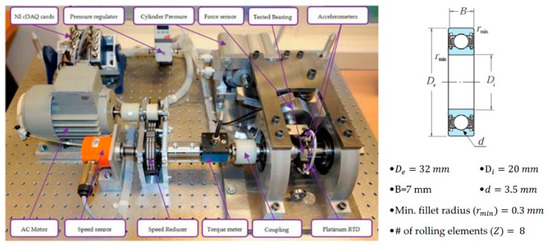
Figure 2.
Detailed labeling of the experimental platform and the ball bearing dimensions.

Table 1.
Technical data of the ball bearings.
2.2. Vibration Data Sets
In this work, accelerated degradation tests were conducted on 17 ball bearings running in the experimental platform PRONOSTIA. There are several conditions that may cause a failure in a bearing, including high running speed and excessive dynamic loading. In these tests, several loads greater than or equal to the maximum dynamic load (4000 N) were applied to different bearings. All the operating conditions of the bearings are shown in Table 2. Since the experimental data are extracted from the laboratory tests instead of the real-life field, the need for different considerations (de-noising, time synchronous averaging, and order tracking) is minimal.
Table 2.
Operating conditions of the different data sets.
All the bearings were running under a radial load greater than or equal to the maximum dynamic load (4000 N) to accelerate the degradation process. Even though several other factors (lubricant degradation, wear debris, high temperature, etc.) may play a role in bearing degradation, especially at the final stage before the failure, the dynamic overloading of the bearing is the dominant factor in the degradation. During these tests, the vibration data of the bearing were only monitored via the horizontal and vertical accelerometers. In the future, it would be interesting to monitor other factors, such as subsurface stresses and lubricant condition [20,21,22], and study their effect on the vibration data.
The vibration data of a rolling bearing can be measured via displacement, velocity, or acceleration sensors. In this paper, the vibration data sets were measured using an accelerometer (DYTRAN 3035B). The sampling rate of the accelerometer was 25.6 kHz and the data were measured for 0.1 s duration every 10 s. The accelerometer is a device capable of measuring bearing vibration using acceleration. The main advantages of the accelerometer are its lightweight and compact design, and wide-range frequency response. However, it is known to have higher sensitivity at high frequencies compared to low frequencies. On the other hand, the anderometer measures bearing vibration using a velocity sensor [23]. It can overcome the accelerometer’s disadvantages by working at low signal magnification and measuring at low frequencies up to 30 Hz [24].
3. Materials and Methods
3.1. DFA Method
Long-range correlation has been proven to exist in various systems from different research fields, including physics [25,26], engineering [27], economy [28], medicine [29], etc. The long-range correlated data possess unique statistical characteristics compared to short-range correlated and uncorrelated data. One of the main features of these data is an autocorrelation function that decays hyperbolically with time. The slow decay of the autocorrelation function shows a significant correlation between the data samples as the lag increases.
Several methods and techniques have been derived to quantify the level of long-range memory in stationary and non-stationary time series. One of the robust methods for non-stationary time series is the DFA method. In [30], the method was first introduced to study the existence of long-range correlations in DNA nucleotides. DFA evaluates the strength of long-range correlations by calculating the scaling exponent (). The steps to compute the scaling exponent () of a time series, , with samples are summarized below:
- Subtract the mean of the time series and compute the integrated time series, , as shown in Equation (1).
- Divide the integrated series into equally spaced boxes, . Inside each box, detrend the series segment by subtracting it from its best linear fit, . Repeat this step for different box sizes ().
- Compute the fluctuation function (), as shown in Equation (2), by finding the RMS value of the detrended time series:
- Plot the fluctuation function (F(n)) versus the box size (n) on log–log scale. The scaling exponent () represents the slope of the best linear fit.
All the steps of the DFA method are shown in Figure 3. The DFA is applied on a simulated series with a scaling exponent equal to 0.6, as shown in Figure 3a. The integrated and detrended time series at a box size of 100 samples are shown in Figure 3b,c. In Figure 3d, the estimated scaling exponent represents the slope of the best linear fit of the fluctuation function versus the box size on a log–log scale. The estimated scaling exponent () is within the accepted margin of error.
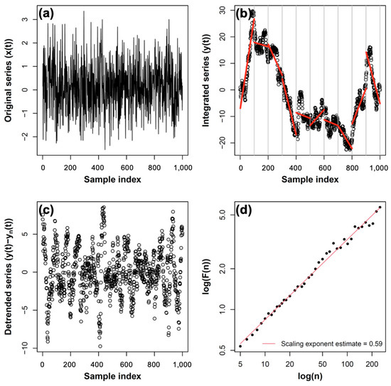
Figure 3.
The steps of the detrended fluctuation analysis (DFA) method: (a) a long-range correlated series (); (b) the integrated series and its best linear fits at samples; (c) the detrended series at samples; (d) the fluctuation function versus the box size.
The scaling exponent () provides a quantitative measure of the degree of long-range correlation in the time series. The long-range correlated time series has a scaling exponent between and . The increases in these series are likely to be followed by further increases and the decreases are likely to be followed by further decreases. For , the time series is called anticorrelated with a decrease expected to follow the increases, and vice versa. The uncorrelated time series has a scaling exponent of 0.5.
3.2. Kendall’s Tau Coefficient
The Kendall’s tau () is a rank correlation coefficient that measures the statistical association between ranked variables. The ranked variables should have ordered and numbered data samples. It is a non-parametric test as it does not rely on any assumptions with respect to the distributions of variables.
For any two variables () and (), the calculation of the coefficient is carried out by counting the number of concordant and discordant pairs, , out of all the possible pair combinations, . A pair is concordant if () and () or () and (). On the other hand, a discordant pair has either () and () or () and (). Any pairs with () or () are not considered in calculating the coefficient. The Kendall’s tau coefficient can be computed using Equation (3).
The Kendall’s tau values vary between −1 and . The positive value (0 < τ < 1) of the coefficient indicates a simultaneous increase in the rank of both variables. The negatively signed coefficients refer to a rank increase in one variable and rank decrease in the other one. A Kendall’s tau close to zero shows no association between the two variables. Three time series with their calculated Kendall’s tau coefficients are shown in Figure 4.
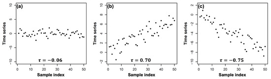
Figure 4.
Three time series with different Kendall’s tau coefficients: (a) ; (b) ; (c) .
4. Results and Discussion
In this paper, a novel approach is proposed to extract the hidden statistical characteristics of the vibration measurements of bearings. As part of the run-to-failure experiment on several bearings, several data sets of horizontal and vertical vibrations signals were collected. DFA can help in understanding the statistical and fractal characteristics of the vibration signals by calculating their scaling exponents (). It is argued that the dynamics of the scaling exponent could provide an early warning for bearing failure.
Evidently, bearing vibrations are non-stationary under normal and faulty operating conditions [31]. The non-stationarity in the time series manifests itself in a time-varying mean and variance over different segments of the series. Since DFA is one of the robust methods to evaluate the long-range correlation in non-stationary data, it was applied to two segments of the vibration signals (horizontal and vertical), as shown in Figure 5. The fluctuation functions in Figure 5b,d have two linear regions with different slopes at the short-range (10–50 samples) and long-range (100–500 samples) scales. This behavior of the fluctuation function is known as the crossover phenomenon [32]. It may result from the sinusoidal trends in the vibrations signals. Moreover, these trends could be the culprit of the proven non-stationarity in the vibration measurements.

Figure 5.
The 2560-sample bearing vibration signals (data set 1_1) and their corresponding fluctuation functions: (a) the bearing vibration signal (2560 samples or 100 ms) on the horizontal axis; (b) the fluctuation function () vs. the box size (n) for the vibration signal on the horizontal axis; (c) the bearing vibration signal (2560 samples or 100 ms) on the vertical axis; (d) the fluctuation Figure 6. smaller time series consisting of 500 segments (5000 s) each, except the last one, which had 300 segments. Then, the scaling exponents ( and ) were estimated for each segment inside these series. The average fluctuation functions inside each of these 6 smaller time series are shown in Figure 6b and Figure 7b. In both figures, the results show a persistent increase in the average scaling exponents () at the short range by moving from the first time series (pink) to the last one (green). Although the average scaling exponents () show a decreasing trend, it will be shown later that the scaling exponent () behaves differently in other data sets.
In the horizontal vibration signal, the scaling exponents at the short range () and long range () were 0.72 and 0.42, respectively. The calculated scaling exponents show that the horizontal signal possessed long-range correlation at the short range, and it was anti-correlated at the long-range scale. On the other hand, the vertical vibration signal had scaling exponents of 0.41 and 0.27 at the short-range and long-range scales, respectively. This signal had anti-correlated behavior on both scales. Even though all the scaling exponents were below 1, similar to the stationary time series (), it is evident that the vibrations signals were non-stationary as a result of the existing trends and the clear crossover phenomenon.
After examining the long-range correlations in the two segments (2560 samples each) of the horizontal and vertical vibration signals, it is important to study the long-range correlations in the complete run-to-failure vibration signals. It would be interesting to see how the evolution of different stages of bearing failure was reflected in scaling exponent dynamics. To that end, the scaling exponents were computed in the complete horizontal and vertical run-to-failure vibration signals from data set 1_1, as shown in Figure 6a and Figure 7a. Each signal consisted of 2800 segments (2560 samples) and total duration of 7.77 h (28,000 s).
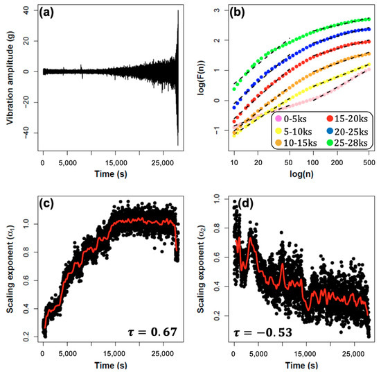
Figure 6.
The horizontal bearing vibration signal (data set 1_1) and its corresponding fluctuation functions and scaling exponents: (a) the horizontal vibration signal; (b) the average fluctuation Figure 1. inside 2560-sample windows of the horizontal vibration signal toward the bearing failure; (d) the scaling exponents ( inside 2560-sample windows of the horizontal vibration signal toward the bearing failure.
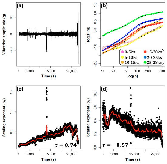
Figure 7.
The vertical bearing vibration signal (data set 1_1) and its corresponding fluctuation functions and scaling exponents: (a) the vertical vibration signal; (b) the average fluctuation function vs. the box size over several segments of the vertical vibration signal; (c) the scaling exponents () inside 2560-sample windows of the vertical vibration signal toward the bearing failure; (d) the scaling exponents () inside 2560-sample windows of the vertical vibration signal toward the bearing failure.
For the horizontal and vertical vibration signals, the means and standard deviations of the scaling exponents ( and ) are shown in Table 3. In the horizontal vibration signal, the average scaling exponent () changed from 0.43 (anticorrelated) at the beginning of the experiment to 0.98 (long-range correlated) before the bearing failure. The change in the scaling exponent () at the short range could be related to a shift in the mechanical system dynamics as part of the run-to-failure experiment. Similarly, in the vertical vibration signal, the average scaling exponent () had a gradual increase with time, starting from 0.18 in the first time series and increasing up to 0.47 in the last time series.
Table 3.
The mean and standard deviation of scaling exponents of the bearing vibration signals (data set 1_1) toward the bearing failure.
In Figure 6c,d and Figure 7c,d, the plots show all the scaling exponents ( and ) over time toward bearing failure for the horizontal and vertical vibration signals. The increase in the scaling exponent () is clear in scaling exponent samples and its smoothed version (red-color line). Using the Kendall’s tau () coefficient, the trend in the scaling exponent () can be quantified by analyzing the statistical association between the scaling exponent and time. The calculated Kendall’s tau coefficients of the scaling exponent () were 0.67 and 0.74 in the horizontal and vertical vibration signals, respectively. Based on the significant values of the Kendall’s tau before bearing failure, it appears that this rise was related to accelerated failure conditions and the proximity to bearing failure. Tracking the Kendall’s tau over time could be an efficient tool in the preventative maintenance field.
Usually, complex and dynamic systems undergo hidden changes as they approach a major critical transition. These changes are known as the critical slowing down phenomenon where the system requires more time to recover from any small disturbance [33]. The slower recovery can be examined in the system state by calculating the lag-1 autocorrelation or the scaling exponent. As the system is approaching the critical transition, it shows a persistent and gradual increase in the autocorrelation and the scaling exponent [34,35]. The critical slowing down could be the culprit of the change in the scaling exponent () before bearing failure. Therefore, the Kendall’s tau of the scaling exponent at the short-range scale could provide a reliable measure of the proximity to bearing failure.
To validate the proposed method, DFA was applied on several vibration signals from 17 data sets to calculate the scaling exponents over all the segments. Then, the trend in the scaling exponent for each vibration signal was examined by calculating the Kendall’s tau coefficient. Table 4 illustrates the Kendall’s tau of the scaling exponents ( and ) for the 17 data sets with a total of 34 horizontal and vertical vibration signals. In addition, the plots of the scaling exponent () for the data sets are shown in Figure 8, Figure 9 and Figure 10.
Table 4.
Kendall’s tau of the scaling exponents ( and ) for several bearing vibration signals toward their failure.
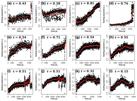
Figure 8.
The scaling exponents () of non-overlapping 2560-sample segments of the vibration signals toward bearing failure: (a) data set 1_2 (horizontal); (b) data set 1_2 (vertical); (c) data set 1_3 (horizontal); (d) data set 1_3 (vertical); (e) data set 1_4 (horizontal); (f) data set 1_4 (vertical); (g) data set 1_5 (horizontal); (h) data set 1_5 (vertical); (i) data set 1_6 (horizontal); (j) data set 1_6 (vertical); (k) data set 1_7 (horizontal); (l) data set 1_7 (vertical).
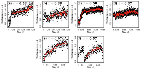
Figure 9.
The scaling exponents () of non-overlapping 2560-sample segments of the vibration signals toward bearing failure: (a) data set 3_1 (horizontal); (b) data set 3_1 (vertical); (c) data set 3_2 (horizontal); (d) data set 3_2 (vertical); (e) data set 3_3 (horizontal); (f) data set 3_3 (vertical).
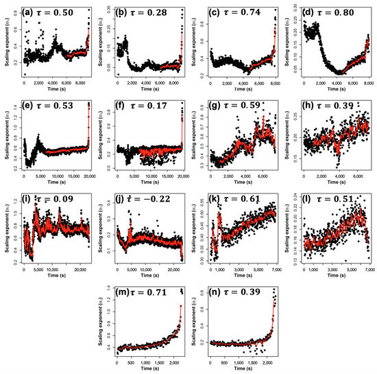
Figure 10.
The scaling exponents () of non-overlapping 2560-sample segments of the vibration signals toward bearing failure: (a) data set 2_1 (horizontal); (b) data set 2_1 (vertical); (c) data set 2_2 (horizontal); (d) data set 2_2 (vertical); (e) data set 2_3 (horizontal); (f) data set 2_3 (vertical); (g) data set 2_4 (horizontal); (h) data set 2_4 (vertical); (i) data set 2_5 (horizontal); (j) data set 2_5 (vertical); (k) data set 2_6 (horizontal); (l) data set 2_6 (vertical); (m) data set 2_7 (horizontal); (n) data set 2_7 (vertical).
The increase in the scaling exponent () is clear from the positive Kendall’s tau coefficients ( for 33 out of the 34 vibration signals. Moreover, 22 vibration signals had a significant rise in the Kendall’s tau coefficient with . That provides strong evidence for the existence of critical slowing down in the vibration signals toward their failure. On the other hand, as mentioned earlier, the scaling exponents () at the long range do not possess a consistent behavior among the different data sets. Some vibration signals have an increasing trend and other signals have a decreasing trend.
Practically, a large portion of machine breakdowns originates from bearing failures; therefore, it is of great importance to monitor bearing condition. The main goals of bearing monitoring are decreasing maintenance cost and maintaining a smooth and continuous running of the system. As part of predictive maintenance, the proposed method can be integrated as a new detection technique in bearing condition monitoring through its vibration measurements.
Moreover, ball bearings are mostly used in low- and medium-speed applications, such as industry, automotive, agriculture, etc. So, the proposed method has the potential to be used in different rotating equipment in the industrial sector (electric motors, pumps, compressors, assembly lines, and elevators) and the automotive sector (engines, steering wheel, driveshaft, driveline, and gearboxes).
5. Conclusions
Using DFA, it was shown that long-range correlations exist in bearing vibration signals before their failure. DFA is a reliable method to quantify the long-range correlations in long time series with a linear fluctuation function at different time scales. In several data sets of bearing vibration signals, the crossover phenomenon emerged with two scaling exponents at the short and long ranges. The estimated short-range scaling exponents showed a persistent and gradual increase toward failure among the different data sets. Then, the Kendall’s tau coefficient was used to measure the trend in the scaling exponents. The results call for adoption of the Kendall’s tau of the scaling exponent as a novel health indicator of the bearings. Furthermore, the proposed method has the potential to be integrated as a new detection technique of bearing failure in condition monitoring systems.
In the future, the effect of other abnormal conditions (lubricant degradation, wear debris, high temperature, etc.) on the vibration signal dynamics will be examined. In addition, it would be interesting to investigate the vibration signals of other elements in mechanical systems using the proposed approach.
Author Contributions
Conceptualization, A.A.; data curation, A.A.; formal analysis, A.A. and L.S.; investigation, A.A.; methodology, L.S.; supervision, L.S.; validation, A.A. and L.S.; writing—original draft, A.A. and L.S.; writing—review and editing, A.A. and L.S. All authors have read and agreed to the published version of the manuscript.
Funding
This research received no external funding.
Acknowledgments
This work is supported by the deanship of scientific research at the German Jordanian University.
Conflicts of Interest
The authors declare no conflict of interest.
Nomenclature
| DFA | Detrended fluctuation analysis |
| EWS | Early warning signal |
| REB | Rolling element bearing |
| PbM | Physics-based model |
| DDM | Data-driven model |
| RMS | Root mean square |
| RUL | Remaining useful life |
| SK | Spectral kurtosis |
| PF | Particle filter |
| VMD | Variational model decomposition |
| Diameter of the outer race | |
| Diameter of the inner race | |
| Number of rolling elements | |
| Diameter of rolling elements | |
| Minimum fillet radius | |
| B | Bearing width |
| Box size | |
| Integrated time series | |
| Best linear fit of time series inside a box of size n | |
| Fluctuation function | |
| Scaling exponent | |
| Short-range scaling exponent | |
| Long-range scaling exponent | |
| Kendall’s tau coefficient |
References
- Atamuradov, V.; Medjaher, K.; Camci, F.; Zerhouni, N.; Dersin, P.; Lamoureux, B. Machine health indicator construction framework for failure diagnostics and prognostics. J. Signal Process. Syst. 2020, 92, 591–609. [Google Scholar] [CrossRef]
- Rezamand, M.; Kordestani, M.; Carriveau, R.; Ting, D.S.-K.; Orchard, M.E.; Saif, M. Critical wind turbine components prognostics: A comprehensive review. IEEE Trans. Instrum. Meas. 2020, 69, 9306–9328. [Google Scholar] [CrossRef]
- Li, X.; Ding, Q.; Sun, J.-Q. Remaining useful life estimation in prognostics using deep convolution neural networks. Reliab. Eng. Syst. Saf. 2018, 172, 1–11. [Google Scholar] [CrossRef]
- Diez-Olivan, A.; del Ser, J.; Galar, D.; Sierra, B. Data fusion and machine learning for industrial prognosis: Trends and perspectives towards Industry 4.0. Inf. Fusion 2019, 50, 92–111. [Google Scholar] [CrossRef]
- Wang, J.; Wen, G.; Yang, S.; Liu, Y. Remaining useful life estimation in prognostics using deep bidirectional LSTM neural network. In Proceedings of the 2018 Prognostics and System Health Management Conference (PHM-Chongqing), Chongqing, China, 26–28 October 2018; pp. 1037–1042. [Google Scholar]
- Yadav, O.P.; Pahuja, G.L. Bearing health assessment using time domain analysis of vibration signal. Int. J. Image Graph. Signal Process. (IJIGSP) 2020, 12, 27–40. [Google Scholar]
- Wang, D.; Tsui, K.; Miao, Q. Prognostics and health management: A review of vibration based bearing and gear health indicators. IEEE Access 2018, 6, 665–676. [Google Scholar] [CrossRef]
- Bao, W.; Tu, X.; Hu, Y.; Li, F. Envelope spectrum L-Kurtosis and its application for fault detection of rolling element bearings. IEEE Trans. Instrum. Meas. 2020, 69, 1993–2002. [Google Scholar] [CrossRef]
- Bastami, A.R.; Bashari, A. Rolling element bearing diagnosis using spectral kurtosis based on optimized impulse response wavelet. J. Vib. Control 2019, 26, 175–185. [Google Scholar] [CrossRef]
- Medjaher, K.; Zerhouni, N.; Baklouti, J. Data-driven prognostics based on health indicator construction: Application to PRONOSTIA’s data. In Proceedings of the 2013 European Control Conference (ECC), Zurich, Switzerland, 17–19 July 2013; pp. 1451–1456. [Google Scholar]
- Li, N.; Lei, Y.; Lin, J.; Ding, S.X. An improved exponential model for predicting remaining useful life of rolling element bearings. IEEE Trans. Ind. Electron. 2015, 62, 7762–7773. [Google Scholar] [CrossRef]
- Wang, P.; Yan, R.; Gao, R.X. Multi-mode particle filter for bearing remaining life prediction. In Proceedings of the International Manufacturing Science and Engineering Conference, College Station, TX, USA, 18–22 June 2018. [Google Scholar]
- Ahmad, W.; Khan, S.; Kim, J.-M. A hybrid prognostics technique for rolling element bearings using adaptive predictive models. IEEE Trans. Ind. Electron. 2018, 65, 1577–1584. [Google Scholar] [CrossRef]
- Singleton, R.K.; Strangas, E.G.; Aviyente, S. Extended Kalman filtering for remaining-useful-life estimation of bearings. IEEE Trans. Ind. Electron. 2015, 62, 1781–1790. [Google Scholar] [CrossRef]
- Soualhi, A.; Medjaher, K.; Zerhouni, N. Bearing health monitoring based on Hilbert-Huang transform, support vector machine and regression. IEEE Trans. Instrum. Meas. 2015, 64, 52–62. [Google Scholar] [CrossRef]
- Hu, S.; Xiao, H.; Yi, C. A novel detrended fluctuation analysis method for gear fault diagnosis based on variational mode decomposition. Shock Vib. 2018, 2018, 1–11. [Google Scholar] [CrossRef]
- Wang, J.; Xiao, H.; Lv, Y.; Wang, T.; Xu, Z. Detrended fluctuation analysis and hough transform based self-adaptation double-scale feature extraction of gear vibration signals. Shock Vib. 2016, 2016, 1–9. [Google Scholar] [CrossRef]
- Lin, J.; Chen, Q. A novel method for feature extraction using crossover characteristics of nonlinear data and its application to fault diagnosis of rotary machinery. Mech. Syst. Signal Process. 2014, 48, 174–187. [Google Scholar] [CrossRef]
- Nectoux, P.; Gouriveau, R.; Medjaher, K.; Ramasso, E.; Chebel-Morello, B.; Zerhouni, N.; Varnier, C. PRONOSTIA: An experimental platform for bearings accelerated degradation tests. In Proceedings of the 2012 IEEE international conference on Prognostics and Health Management, Denver, CO, USA, 18–21 June 2012; pp. 1–8. [Google Scholar]
- Johns-Rahnejat, P.M.; Dolatabadi, N.; Rahnejat, H. Analytical elastostatic contact mechanics of highly-loaded contacts of varying conformity. Lubricants 2020, 8, 89. [Google Scholar] [CrossRef]
- Okamoto, Y.; Kitahara, K.; Ushijima, K.; Aoyama, S.; Xu, H.; Jones, G.J. A study for wear and fatigue on engine bearings by using EHL analysis. JSAE Rev. 2000, 21, 189–196. [Google Scholar] [CrossRef]
- Gabelli, A.; Morales-Espejel, G.E.; Ioannides, E. Particle damage in Hertzian contacts and life ratings of rolling bearings. Tribol. Trans. 2008, 51, 428–445. [Google Scholar] [CrossRef]
- Adamczak, S.; Zmarzły, P. Research of the influence of the 2D and 3D surface roughness parameters of bearing raceways on the vibration level. J. Phys. Conf. Ser. 2019, 1183, 1–10. [Google Scholar] [CrossRef]
- Adamczak, S.; Zmarzły, P. Influence of raceway waviness on the level of vibration in rolling-element bearings. Bull. Polish Acad. Sci. Tech. Sci. 2017, 65, 541–551. [Google Scholar] [CrossRef]
- Xia, H.; Tang, G.; Lan, Y. Long-range temporal correlations in kinetic roughening. J. Stat. Phys. 2020, 178, 800–813. [Google Scholar] [CrossRef]
- Martin-Montoya, L.A.; Aranda-Camachob, N.M.; Quimbay, C.J. Long-range correlations and trends in Colombian seismic time series. Phys. A Stat. Mech. Appl. 2015, 421, 124–133. [Google Scholar] [CrossRef]
- Shalalfeh, L.; Bogdan, P.; Jonckheere, E. Evidence of long-range dependence in power grid. In Proceedings of the IEEE Power and Energy Society General Meeting (PESGM), Boston, MA, USA, 17–21 July 2016; pp. 1–5. [Google Scholar]
- Mariani, M.C.; Asante, P.; Bhuiyan, M.A.M.; Beccar-Varela, M.P.; Sebastian, J.; Tweneboah, O.K. Long-range correlations and characterization of financial and volcanic time series. Mathematics 2020, 8, 441. [Google Scholar] [CrossRef]
- Nakata, A.; Kaneko, M.; Evans, N.; Shigematsu, T.; Kiyono, K. Long-range cross-correlation between heart rate and physical activity in daily life. In Proceedings of the 11th Conference of the European Study Group on Cardiovascular Oscillations (ESGCO), Pisa, Italy, 15 July 2020; pp. 1–2. [Google Scholar]
- Peng, C.-K.; Buldyrev, S.V.; Havlin, S.; Simons, M.; Stanley, H.; Goldberger, A.L. Mosaic organization of DNA nucleotides. Phys. Rev. E 1994, 49, 1685–1689. [Google Scholar] [CrossRef]
- Gao, R.; Yan, R. Non-stationary signal processing for bearing health monitoring. Int. J. Manuf. Res. 2006, 1, 18–40. [Google Scholar] [CrossRef]
- Hu, K.; Ivanov, P.; Chen, Z.; Carpena, P.; Stanley, H. Effect of Trends on Detrended Fluctuation Analysis. Phys. Rev. E Stat. Nonlinear Soft Matter Phys. 2001, 64, 011114. [Google Scholar] [CrossRef]
- Nes, E.; Scheffer, M. Slow Recovery from Perturbations as a Generic Indicator of a Nearby Catastrophic Shift. Am. Nat. 2007, 169, 738–747. [Google Scholar]
- Held, H.; Kleinen, T. Detection of climate system bifurcations by degenerate fingerprinting. Geophys. Res. Lett. 2004, 31, L23207. [Google Scholar] [CrossRef]
- Shalalfeh, L.; Bogdan, P.; Jonckheere, E. Kendall’s tau of frequency Hurst exponent as blackout proximity Margin. In Proceedings of the 2016 IEEE International Conference on Smart Grid Communications (SmartGridComm), Sydney, Australia, 6–9 November 2016; pp. 466–471. [Google Scholar]


Publisher’s Note: MDPI stays neutral with regard to jurisdictional claims in published maps and institutional affiliations. |
© 2020 by the authors. Licensee MDPI, Basel, Switzerland. This article is an open access article distributed under the terms and conditions of the Creative Commons Attribution (CC BY) license (http://creativecommons.org/licenses/by/4.0/).