Estimating Cycling Aerodynamic Performance Using Anthropometric Measures

 , ,
, ,
Abstract
:1. Introduction
2. Materials and Methods
2.1. Participants
2.2. Optical Mocap
2.3. Inertial Mocap
2.4. Protocol
- Static protocol, where the instruction was to maintain three poses (Figure 3) for at least five seconds each, with the right leg extended to the bottom of the pedal stroke:
- Time Trial (TT): race pose with arms resting horizontally on the clip-on handlebars;
- Hoods: relaxed pose with hands on the hoods of the handlebar; and
- Drops: race pose with hands on the dropped handlebars.
- 2.
- Dynamic protocol, which lasted roughly two minutes per participant. The cyclists were instructed to pedal at a cadence of roughly 1 Hz and position their hands on the handlebar hoods and:
- bend their back from the highest possible to lowest possible inclination and back over 30 s;
- pronate knees from closest to farthest from top tube and back over 30 s;
- extend neck from lowest possible to highest possible angle and back over 30 s; and
- proceed to perform 30 s of comfortable cycling.
2.5. Procedure
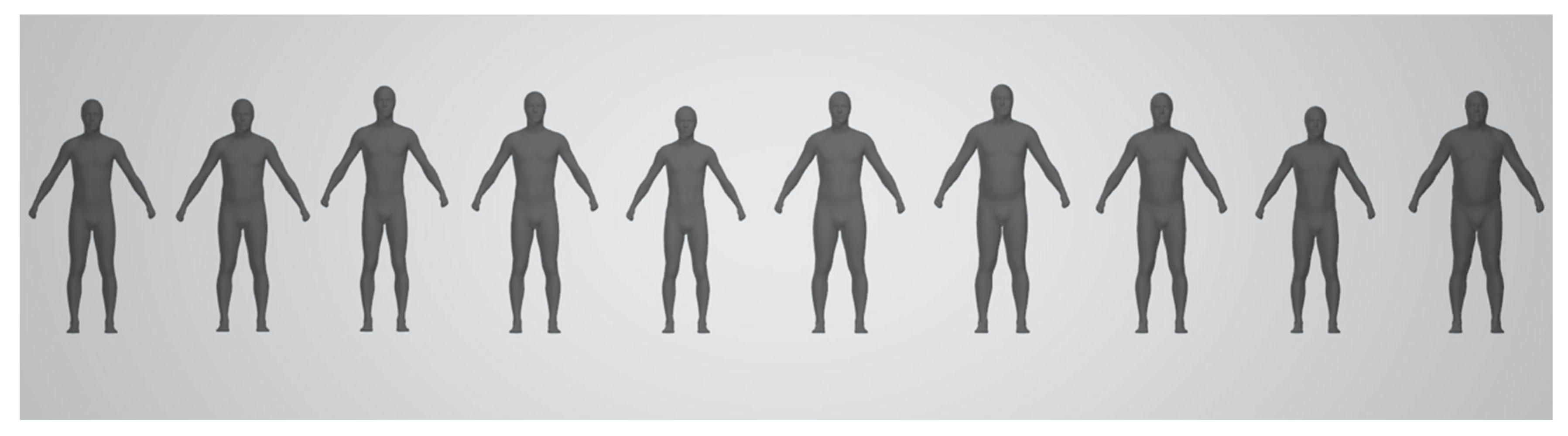
2.5.1. 3D Models
2.5.2. Computational Fluid Dynamics (CFD) Analysis
2.5.3. Regression Analyses
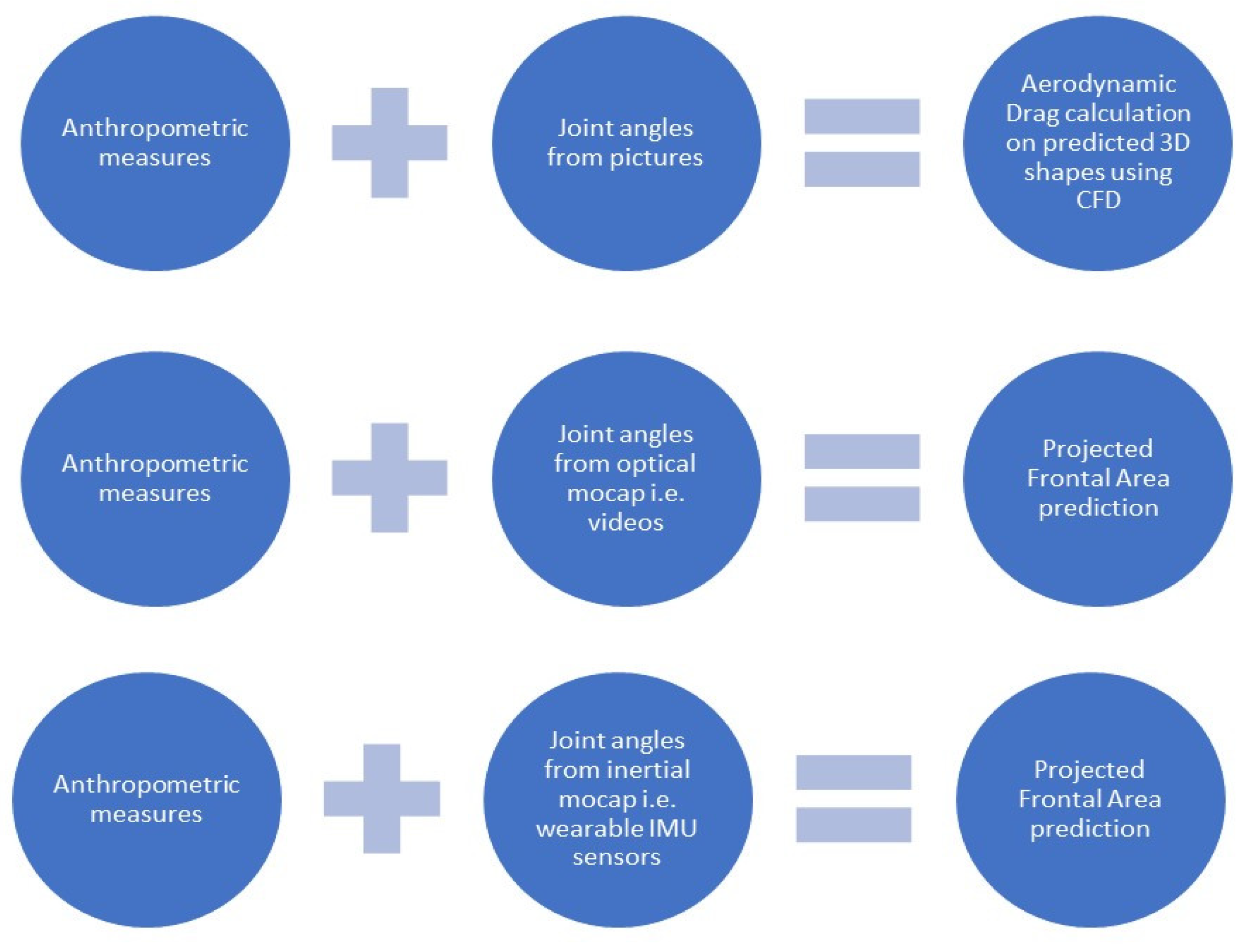
- (1)
- (2)
- anthropometric data and joint angles from the inertial mocap system (Table 1).
3. Results
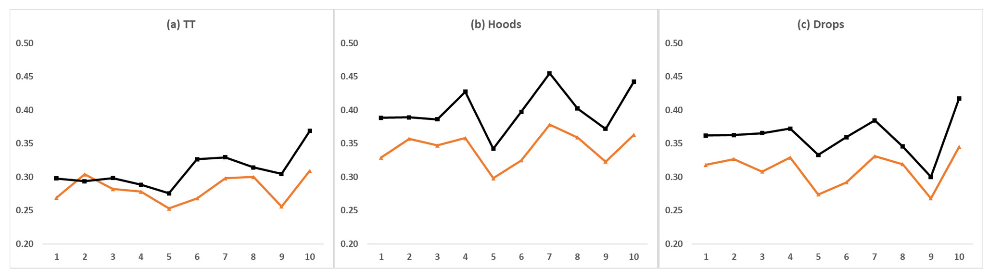
3.1. Drag Force versus Projected Frontal Area
3.2. Projected Frontal Area Prediction Based on Anthropometrics and Joint Angles
4. Discussion
4.1. Drag Force versus Projected Frontal Area
4.2. Projected Frontal Area Prediction Based on Anthropometrics and Joint Angles
5. Conclusions
Author Contributions
Funding
Conflicts of Interest
References
- Blocken, B.; van Druenen, T.; Toparlar, Y.; Andrianne, T. Aerodynamic analysis of different cyclist hill descent positions. J. Wind Eng. Ind. Aerodyn. 2018, 181, 27–45. [Google Scholar] [CrossRef]
- Ainegren, M.; Jonsson, P. Drag Area, Frontal Area and Drag Coefficient in Cross-Country Skiing Techniques. Proceedings 2018, 2, 313. [Google Scholar] [CrossRef] [Green Version]
- Martin, J.C.; Milliken, D.L.; Cobb, J.E.; McFadden, K.L.; Coggan, A.R. Validation of a mathematical model for road cycling power. J. Appl. Biomech. 1998, 14, 276–291. [Google Scholar] [CrossRef] [Green Version]
- Merkes, P.F.J.; Menaspà, P.; Abbiss, C.R. Validity of the Velocomp powerpod compared with the verve cycling infocrank power meter. Int. J. Sports Physiol. Perform. 2019, 14, 1382–1387. [Google Scholar] [CrossRef]
- Valenzuela, P.L.; Alcalde, Y.; Gil-Cabrera, J.; Talavera, E.; Lucia, A.; Barranco-Gil, D. Validity of a novel device for real-time analysis of cyclists’ drag area. J. Sci. Med. Sport 2020, 23, 421–425. [Google Scholar] [CrossRef]
- Íñiguez-De-La Torre, A.; Íñiguez, J. Aerodynamics of a cycling team in a time trial: Does the cyclist at the front benefit? Eur. J. Phys. 2009, 30, 1365–1369. [Google Scholar] [CrossRef]
- Fintelman, D.M.; Hemida, H.; Sterling, M.; Li, F.X. CFD simulations of the flow around a cyclist subjected to crosswinds. J. Wind Eng. Ind. Aerodyn. 2015, 144, 31–41. [Google Scholar] [CrossRef] [Green Version]
- Defraeye, T.; Blocken, B.; Koninckx, E.; Hespel, P.; Carmeliet, J. Computational fluid dynamics analysis of cyclist aerodynamics: Performance of different turbulence-modelling and boundary-layer modelling approaches. J. Biomech. 2010, 43, 2281–2287. [Google Scholar] [CrossRef] [PubMed] [Green Version]
- Godo, M.; Corson, M.; Legensky, S. An Aerodynamic Study of Bicycle Wheel Performance Using CFD. In Proceedings of the 47th AIAA Aerospace Sciences Meeting Including the New Horizons Forum and Aerospace Exposition, Orlando, FL, USA, 5–8 January 2009. [Google Scholar] [CrossRef] [Green Version]
- Godo, M.; Corson, D.; Legensky, S. A Comparative Aerodynamic Study of Commercial Bicycle Wheels Using CFD. In Proceedings of the 48th AIAA Aerospace Sciences Meeting Including the New Horizons Forum and Aerospace Exposition, Orlando, FL, USA, 4–7 January 2010. [Google Scholar] [CrossRef] [Green Version]
- Blocken, B.; Toparlar, Y. A following car influences cyclist drag: CFD simulations and wind tunnel measurements. J. Wind Eng. Ind. Aerodyn. 2015, 145, 178–186. [Google Scholar] [CrossRef] [Green Version]
- Blocken, B.; van Druenen, T.; Toparlar, Y.; Malizia, F.; Mannion, P.; Andrianne, T.; Marchal, T.; Maas, G.J.; Diepens, J. Aerodynamic drag in cycling pelotons: New insights by CFD simulation and wind tunnel testing. J. Wind Eng. Ind. Aerodyn. 2018, 179, 319–337. [Google Scholar] [CrossRef]
- Blocken, B.; Toparlar, Y.; Andrianne, T. Aerodynamic benefit for a cyclist by a following motorcycle. J. Wind Eng. Ind. Aerodyn. 2016, 155, 1–10. [Google Scholar] [CrossRef] [Green Version]
- Huysmans, T.; Goto, L.; Molenbroek, J.; Goossens, R. DINED Mannequin. Tijdschr. Voor Hum. Factors 2020, 45, 4–7. [Google Scholar]
- Ballester, A.I.; Piérola, A.; Parrilla, E.; Uriel, J.; Ruescas, A.V.; Perez, C.; Durá, J.V.; Alemany, S. 3D Human Models from 1D, 2D and 3D Inputs: Reliability and Compatibility of Body Measurements. In Proceedings of the 9th International Conference on 3D Body Scanning Technologies, Lugano, Switzerland, 16–17 October 2018. [Google Scholar] [CrossRef] [Green Version]
- Ballester, A.; Parrilla, E.; Vivas, J.A.; Pierola, A.; Uriel, J.; Puigcerver, S.A.; Piqueras, P.; Solve, C.; Rodriguez, M.; Gonzalez, J.C.; et al. Low-cost data-driven 3D reconstruction and its applications. In Proceedings of the 6th International Conference on 3D Body Scanning Technologies, Lugano, Switzerland, 27–28 October 2015. [Google Scholar] [CrossRef] [Green Version]
- Allen, B.; Curless, B.; Popović, Z. Exploring the Space of Human Body Shapes: Data-driven Synthesis under Anthropometric Control. Sae Int. 2004. [Google Scholar] [CrossRef] [Green Version]
- Stave, D.Å. Cyclist Posture Optimisation Using CFD. 2018. Available online: https://brage.bibsys.no/xmlui/handle/11250/2562590?platform=hootsuite (accessed on 27 November 2020).
- Garimella, R.; Beyers, K.; Huysmans, T.; Verwulgen, S. Rigging and Re-posing a Human Model from Standing to Cycling Configuration. In International Conference on Applied Human Factors and Ergonomics; Springer: Cham, Switzerland; Washington, DC, USA, 2019; pp. 525–532. [Google Scholar] [CrossRef]
- Defraeye, T.; Blocken, B.; Koninckx, E.; Hespel, P.; Carmeliet, J. Aerodynamic study of different cyclist positions: CFD analysis and full-scale wind-tunnel tests. J. Biomech. 2010, 43, 1262–1268. [Google Scholar] [CrossRef] [Green Version]
- Debraux, P.; Grappe, F.; Manolova, A.V.; Bertucci, W. Aerodynamic drag in cycling: Methods of assessment. Sport. Biomech. 2011, 10, 197–218. [Google Scholar] [CrossRef]
- Heil, D.P. Body mass scaling of projected frontal area in competitive cyclists. Eur. J. Appl. Physiol. 2001, 85, 358–366. [Google Scholar] [CrossRef]
- Olds, T.; Olive, S. Methodological considerations in the determination of projected frontal area in cyclists. J. Sports Sci. 1999, 17, 335–345. [Google Scholar] [CrossRef]
- Debraux, P.; Bertucci, W.; Manolova, A.V.; Rogier, S.; Lodini, A. New method to estimate the cycling frontal area. Int. J. Sports Med. 2009, 30, 266–272. [Google Scholar] [CrossRef]
- Barelle, C.; Chabroux, V.; Favier, D. Modeling of the time trial cyclist projected frontal area incorporating anthropometric, postural and helmet characteristics. Sport Eng. 2010, 12, 199–206. [Google Scholar] [CrossRef]
- Danckaers, F.; Huysmans, F.; Lacko, D.; Sijbers, J. Evaluation of 3D Body Shape Predictions Based on Features. In Proceedings of the Proceedings of the 6th International Conference on 3D Body Scanning Technologies, Lugano, Switzerland, 27–28 October 2015; pp. 258–265. [Google Scholar] [CrossRef] [Green Version]
- Garimella, R.; Peeters, T.; Beyers, K.; Truijen, S.; Huysmans, T.; Verwulgen, S. Capturing Joint Angles of the Off-Site Human Body; IEEE: New Delhi, India, 2018; pp. 1244–1247. [Google Scholar] [CrossRef]
- Smith, M.F.; Davison, R.C.R.; Balmer, J.; Bird, S.R. Reliability of mean power recorded during indoor and outdoor self-paced 40 km cycling time-trials. Int. J. Sports Med. 2001, 22, 270–274. [Google Scholar] [CrossRef]
- Griffith, M.D.; Crouch, T.; Thompson, M.C.; Burton, D.; Sheridan, J.; Brown, N.A.T. Computational Fluid Dynamics Study of the Effect of Leg Position on Cyclist Aerodynamic Drag. J. Fluids Eng. 2014, 136, 101105. [Google Scholar] [CrossRef] [Green Version]
- Celis, B.; Ubbens, H.H. Design and Construction of an Open-circuit Wind Tunnel with Specific Measurement Equipment for Cycling. Procedia Eng. 2016, 147, 98–103. [Google Scholar] [CrossRef] [Green Version]
- Weir, J. Quantifying test-retest reliability using the intraclass correlation coefficient and the SEM. J. Strength Cond Res. 2005, 19, 231–240. [Google Scholar]
- Hawkins, D.M.; Basak, S.C.; Mills, D. Assessing Model Fit by Cross-Validation. J. Chem. Inf. Model. 2003, 43, 579–586. [Google Scholar] [CrossRef]
- Barry, N.; Burton, D.; Sheridan, J.; Thompson, M.; Brown, N.A.T. Aerodynamic performance and riding posture in road cycling and triathlon. J. Spors Eng. Technol. 2015, 229, 28–38. [Google Scholar] [CrossRef]
- Bogo, F.; Kanazawa, A.; Lassner, C.; Gehler, P.; Romero, J.; Black, M.J. Keep it SMPL: Automatic estimation of 3D human pose and shape from a single image. In European Conference on Computer Vision; Springer: Amsterdam, The Netherlands; Cham, Switzerland, 2016; Volume 9909, pp. 561–578. [Google Scholar] [CrossRef] [Green Version]
- Black, M.J. Estimating Human Motion: Past, Present, and Future. Talk. October 2018. Available online: https://www.youtube.com/watch?v=5jU9rIqBz7M (accessed on 27 November 2020).
- Bogo, F.; Romero, J.; Loper, M.; Black, M.J. FAUST: Dataset and evaluation for 3D mesh registration. In Proceedings of the IEEE Conference on Computer Vision and Pattern Recognition, Columbus, OH, USA, 23–28 June 2014; pp. 3794–3801. [Google Scholar] [CrossRef] [Green Version]
- Pons-Moll, G.; Romero, J.; Mahmood, N.; Black, M.J. Dyna: A model of dynamic human shape in motion. ACM Trans. Graph. 2015, 34, 4. [Google Scholar] [CrossRef]
- Peeters, T.; Garimella, R.; Francken, E.; Henderieckx, S.; van Nunen, L.; Verwulgen, S. The Correlation between Frontal Area and Joint Angles During Cycling. Adv. Intell. Syst. Comput. 2020, 1206, 251–258. [Google Scholar] [CrossRef]
- Fintelman, D.M.; Sterling, M.; Hemida, H.; Li, F.X. Optimal cycling time trial position models: Aerodynamics versus power output and metabolic energy. J. Biomech. 2014, 47, 1894–1898. [Google Scholar] [CrossRef] [PubMed]
- Smurthwaite, J. How to Be More Aero on Your Road Bike (Video), Cycling Weekly. 2015. Available online: https://www.cyclingweekly.com/videos/fitness/be-faster-by-being-more-aero (accessed on 25 November 2020).
- Airshaper—Aerodynamics Made Easy. Available online: www.airshaper.com (accessed on 27 November 2020).
- Bioracer Aero. Available online: https://bioracermotion.com/en/bioracer-aero (accessed on 10 May 2020).


| Anthropometric Data (cm) | 2D Joint Angles Optical Mocap (°) | 3D Joint Angles Inertial Mocap (°) | |
|---|---|---|---|
| Body Height | Shoulder Breadth (acromion) | Left Knee | Left Knee |
| Chest Circumference | Hip Breadth (standing) | Left Elbow | Left Shoulder |
| Under-Bust Circumference | Chest Circumference (scye) | Left Hip | Left Elbow |
| Waist Circumference (minimum) | Hip Circumference | Back | Right Knee |
| Waist Circumference (trousers) | Arm Circumference (scye) | Head | Right Shoulder |
| Neck Circumference (shirt) | Shoulder Breadth (bideltoid) | Left Shoulder | Right Elbow |
| Neck Circumference (tight, hull) | Hip Breadth (sitting) | Neck (2D) | |
| Lower Arm Circumference (mid, Hull) | Upper Arm Length | Left Hip | |
| Biceps Circumference Hull | Lower Arm Length | Right Hip | |
| Spine-Shoulder Length | Sternum to Femur Length | Pelvis | |
| Arm Length | Upper Leg Length | Left Wrist | |
| Back Length (shirt) | Lower Leg Length | Right Wrist | |
| Torso Length (shirt) | Body Mass (kg) | Chest | |
| Age (years) | Gender (m/f) | ||
| Parameter | Value |
|---|---|
| Air Viscosity | 1.81 × 10⁻⁵ Pa∙s |
| Inlet Velocity/ Air Speed U∞ (free stream) | 16.7 m/s = 60 km/h |
| Outlet Pressure | 0 Pa (static) |
| Temperature | 295.3 K |
| Relative Humidity | 39.9 % |
| Atmospheric Pressure | 100,480 Pa |
| Saturation Vapor Pressure | 269,225.2 Pa |
| Air Density | 1.181 kg/m³ |
| Turbulence Model | Shear Stress Transport (SST) k-ω |
| Meshers | Polyhedral |
| Surface Remesher | |
| Prism Layer Mesher | |
| Base Cell Size | 0.15 m |
| Prism Layers | 5 |
| Reynolds number Re | 1.33 × 10⁶ |
| L (dimension of object) | <1 m |
| C, f (skin friction coefficient) | 3.46 × 10⁻³ |
| Wall Shear Stress τ | 2.84 × 10⁻¹ m/s |
| U* (dimensionless velocity) | 4.91 × 10⁻¹ m/s |
| Y (first layer cell height) | 0.00281304 m |
| Y+ | 90 |
| δ (prism layer height) | 0.039 m |
| Participant | 1 | 2 | 3 | 4 | 5 | 6 | 7 | 8 | 9 | 10 | |
|---|---|---|---|---|---|---|---|---|---|---|---|
| TT | Drag (N) | 28.79 | 26.81 | 27.49 | 26.94 | 26.84 | 29.59 | 31.30 | 28.71 | 29.86 | 35.71 |
| CD | 0.70 | 0.58 | 0.64 | 0.63 | 0.69 | 0.72 | 0.69 | 0.63 | 0.76 | 0.76 | |
| Hoods | Drag (N) | 37.43 | 35.99 | 37.31 | 44.23 | 31.80 | 39.07 | 45.03 | 36.13 | 35.97 | 41.67 |
| CD | 0.74 | 0.66 | 0.70 | 0.81 | 0.70 | 0.79 | 0.78 | 0.66 | 0.73 | 0.75 | |
| Drops | Drag (N) | 32.29 | 33.15 | 32.40 | 32.56 | 30.07 | 33.99 | 35.08 | 31.32 | 25.99 | 40.01 |
| CD | 0.66 | 0.66 | 0.69 | 0.65 | 0.72 | 0.76 | 0.69 | 0.64 | 0.63 | 0.76 |
| Optical Regression | Inertial Regression | ||
|---|---|---|---|
| Variable | Beta coefficient | Variable | Beta coefficient |
| Back angle | 0.19 | Neck circumference (tight) | 0.79 |
| Score 6 | 0.49 | Chest anterior tilt | −0.80 |
| Upper arm length | 0.31 | Neck flexion | −0.31 |
| Left elbow flexion | 0.23 | shoulder breadth (acromion) | 0.18 |
| Neck circumference (tight) | 0.12 | Lower arm length | 0.31 |
| Head flexion | −0.12 | Chest lateral tilt | 0.44 |
| Hip Breadth (while sitting) | −0.31 | Upper leg length | 0.66 |
| Left hip flexion | 0.36 | Left elbow flexion | 0.32 |
| Left knee flexion | 0.17 | Right knee flexion | −0.20 |
| Lower arm length | −0.13 | Left knee flexion | −0.30 |
| Left shoulder flexion | 0.09 | Back length | −0.52 |
| Chest rotation | 0.35 | ||
| Right shoulder flexion | −0.27 | ||
| Right elbow supination | 0.34 | ||
| Neck circumference (shirt) | 0.13 | ||
| Left shoulder internal rotation | 0.16 | ||
| Right shoulder internal rotation | 0.09 | ||
| Optical Regression | Inertial Regression | |
|---|---|---|
| ICC | 0.43 (p < 0.001) | 0.51 (p < 0.001) |
| RMSE (m2) | 0.037 | 0.032 |
| Relative error (%) | −0.18 ± 9.98 | 1.70 ± 8.72 |
Publisher’s Note: MDPI stays neutral with regard to jurisdictional claims in published maps and institutional affiliations. |
© 2020 by the authors. Licensee MDPI, Basel, Switzerland. This article is an open access article distributed under the terms and conditions of the Creative Commons Attribution (CC BY) license (http://creativecommons.org/licenses/by/4.0/).
Share and Cite
Garimella, R.; Peeters, T.; Parrilla, E.; Uriel, J.; Sels, S.; Huysmans, T.; Verwulgen, S. Estimating Cycling Aerodynamic Performance Using Anthropometric Measures. Appl. Sci. 2020, 10, 8635. https://doi.org/10.3390/app10238635
Garimella R, Peeters T, Parrilla E, Uriel J, Sels S, Huysmans T, Verwulgen S. Estimating Cycling Aerodynamic Performance Using Anthropometric Measures. Applied Sciences. 2020; 10(23):8635. https://doi.org/10.3390/app10238635
Chicago/Turabian StyleGarimella, Raman, Thomas Peeters, Eduardo Parrilla, Jordi Uriel, Seppe Sels, Toon Huysmans, and Stijn Verwulgen. 2020. "Estimating Cycling Aerodynamic Performance Using Anthropometric Measures" Applied Sciences 10, no. 23: 8635. https://doi.org/10.3390/app10238635
APA StyleGarimella, R., Peeters, T., Parrilla, E., Uriel, J., Sels, S., Huysmans, T., & Verwulgen, S. (2020). Estimating Cycling Aerodynamic Performance Using Anthropometric Measures. Applied Sciences, 10(23), 8635. https://doi.org/10.3390/app10238635