A New Big Data Benchmark for OLAP Cube Design Using Data Pre-Aggregation Techniques

Abstract

In recent years, several new technologies have enabled OLAP processing over Big Data sources. Among these technologies, we highlight those that allow data pre-aggregation because of their demonstrated performance in data querying. This is the case of Apache Kylin, a Hadoop based technology that supports sub-second queries over fact tables with billions of rows combined with ultra high cardinality dimensions. However, taking advantage of data pre-aggregation techniques to designing analytic models for Big Data OLAP is not a trivial task. It requires very advanced knowledge of the underlying technologies and user querying patterns. A wrong design of the OLAP cube alters significantly several key performance metrics, including: (i) the analytic capabilities of the cube (time and ability to provide an answer to a query), (ii) size of the OLAP cube, and (iii) time required to build the OLAP cube. Therefore, in this paper we (i) propose a benchmark to aid Big Data OLAP designers to choose the most suitable cube design for their goals, (ii) we identify and describe the main requirements and trade-offs for effectively designing a Big Data OLAP cube taking advantage of data pre-aggregation techniques, and (iii) we validate our benchmark in a case study.

1. Introduction

Nowadays there is a large number of technologies that enables effective processing of Big Data, i.e., huge data volumes (terabytes), from a diversity of data sources (relational and not relational data) and that are increasingly acquired and processed in real-time. Among the Big Data applications we can implement with these Big Data technologies, Business Intelligence (BI) applications are the most demanded by enterprises. With BI applications we can extract useful insights from the data that can be used for improving decisions processes. Due to this fact, BI systems are often very profitable for organizations.

The main BI applications are report generation, dashboarding, and multidimensional views. However, these applications often require very low query latency, from milliseconds to a few seconds of execution in order to retrieve results from the analytic model. This low query latency is necessary to support interactive BI applications, that promote the discovery of insights by decision makers and data analysts. These kind of interactive BI applications are also known as On-Line Analytical Processing (OLAP). In order to implement OLAP systems, we use the consolidated Data Warehousing techniques [1] that are based on the division of the problem domain in facts (measures for analysis) and dimensions (analysis contexts) around which the analysis of the data is structured.

Nonetheless, in Big Data scenarios where fact tables can have up to billions of rows, the relational database management systems (RDBMS) are not capable of processing them, much less maintaining sub-second query latency. For these cases, distributed storage and processing typically found in Big Data approaches are better suited. Due to this fact, in recent years, Big Data OLAP applications have been gaining attention in the scientific community as it is demonstrated by a number of presented approaches [2,3,4,5,6,7,8]. Among the different OLAP approaches that use Big Data technology for its implementation, we can highlight those that enable data pre-aggregation or indexing to significantly improve performance in data querying. This is the case of Apache Kylin [2,3] and Druid [6], two of the most consolidated Big Data OLAP approaches. Both approaches are based on data pre-aggregation for OLAP cube generation and, thanks to this approach, are able to handle fact tables with up to tens of billions of rows, ultra high cardinality dimensions (more than 300,000 instances of dimensions) and OLAP scenarios both in batch and (near) real-time. While Kylin allows the implementation of very rich multidimensional (MD) analytical models composed of multiple tables (e.g., star or snowflake schemas), Druid does not, as it requires that all data be combined and stored into a single table. However, because the Druid architecture supports data indexing in addition to data pre-aggregation, it is faster than Kylin in real-time scenarios and also for running queries that apply filtering. However, we can also integrate [9] Kylin and Druid, using Druid as an alternative storage to HBase, the default storage for Kylin cubes. As demonstrated in a real case [9], this integration allows for complex schemas and SQL queries (Kylin), while improving the performance of these queries and data loading processes (Druid). In addition to Kylin and Druid, there are other Big Data OLAP tools that support pre-aggregation (e.g., Vertica, Clickhouse, Google Big Query) or indexing (e.g., Elasticsearch, Clickhouse), but are not as efficient in query execution [4,7,8], or do not support very complex data models [5].

Despite the advances in Big Data OLAP technology applying data pre-aggregation, one of the main problems when using any of the above approaches is how to effectively design and implement the analytical data models, also called OLAP cubes. The OLAP cube design requires very advanced knowledge of the underlying technologies. For example, in the case of Apache Kylin, we require advanced knowledge about cube building engine and cube query engine, but also of the underlying Hadoop technologies: Map Reduce, Hive, HBase and, recently added, Spark and Kafka. A wrong cube design can affect some important design goals, such as OLAP cube size, building time or query latency. Due to the importance of these variables, in this paper we propose a benchmark to aid Big Data OLAP designers to choose the most suitable cube design for their goals, also taking advantage of the data pre-aggregation techniques. Moreover, in order to demonstrate the utility of the proposed benchmark, we applied it for Apache Kylin cube design, one of the most powerful and consolidated Big Data OLAP approaches.

In the next section, we review the Big Data approaches for OLAP analytics and discuss various previous benchmarking efforts, that have contributed to our current understanding of Big Data and OLAP benchmarking. In Section 3, we present our proposed benchmark for Big Data OLAP systems and cube design fundamentals for its application to Apache Kylin. Then, in Section 4, we execute the benchmark for the Apache Kylin case. Next, in Section 5, we analyze the execution results. Using the insights extracted from them, we propose a guideline for the effective design of the OLAP cubes. Moreover, we discuss the applicability of our proposed benchmark to other Big Data OLAP approaches and summarize the contributions of our proposal. We conclude in Section 6 after summarizing future work.

2. Related Work

Big Data OLAP techniques [2,3,4,5,6] has become a rich field of study in recent years due to increase of Big Data scenarios and limitations of using RDBMS for fact tables with up to tens of billions of rows. One of the most consolidated and powerful technologies for OLAP with Big Data sources is Apache Kylin [2,3]. It is based on the use of pre-aggregation techniques for reducing query latency over up to billions of rows fact tables, generating a pre-aggregated data structure also called OLAP cube that can be queried with Standard Query Language (SQL). However, in cases where we can tolerate a higher querying latency or have a lower data volume in the fact table, Vertica, Clickhouse or Big Query [4,7,8] are also a good choice. Like Kylin, these approaches implement a distributed and columnar approach and support pre-aggregation techniques. However, the pre-aggregations techniques that they allow are less aggressive than those used by Kylin. This is because data pre-aggregation is not applied by default to most of the data model, but rather the user has to consciously implement and use pre-aggregation at table level. The OLAP cubes generated are usually much smaller than those generated using Kylin, because it is not necessary to store all the possible aggregations and combinations between the facts and the dimension columns. However, thanks the extensive application of data pre-aggregation in the data model, the query execution performance in Kylin is much higher than the other approaches. Another point to consider, is that approaches such as Vertica or Clickhouse require a deeper knowledge of the underlying columnar approach, while Kylin generates the OLAP cube based on a simplified metadata design, abstracting the user from the underlying column storage in Apache HBase. Other Big Data OLAP approaches are Druid [6] and Elasticsearch [5]. Druid supports OLAP analytics over real-time data just in milliseconds after it is acquired, thanks to a distributed architecture that combines memory and disk. Elascticsearch is a consolidated search engine based on a distributed document index. While Kylin cube building process take at least few minutes, in these approaches real-time data are ready for OLAP queries just in millisecond. However, Druid and Elascticsearch have less flexibility than Kylin or Vertica to implement complex analytics models, e.g., using dimensions composed by more than one concept at different level of aggregation, a typical scenario in most OLAP applications. For the above reasons, we consider Apache Kylin the most powerful and flexible Big Data OLAP approach, thus we decided to use it (i) to analyze OLAP cube design process, and (ii) to implement our proposed benchmark.

Regarding the benchmarking approaches for Big Data OLAP systems, in [10], the author proposes a benchmark based on TPC-H Benchmark [11], a consolidated Data Warehousing systems benchmark. The proposed benchmark is executed over Big Data OLAP architecture based on the use of Apache Pig, a Hadoop tool that uses Map Reduce. Despite this approach contribution, we found that the proposed benchmark architecture is not best suited for Big Data OLAP, due to the high latency of Map Reduce processing. Moreover, TPC-H benchmark is only aimed to benchmark query latency over a fixed schema design. We consider this provided schema could be optimal for one database but not for all, especially in case of Big Data OLAP where the data structures supported differ a lot between approaches. Another disadvantage of the TPC-H benchmark is that the proposed data model is fully normalized (3FN), a standardized form for transactional systems and less suitable to implement analytical systems due to its performance penalization.

For this reason, later benchmarks such as SSB [12], TPC-DS [13] and TPCx-BB [14] propose the use of star or snowflake schemes, more suitable [1] for systems that support OLAP applications. In [15], the authors apply the SSB benchmark on Apache Druid [6], where they test different implementations of the data model proposed by SSB. Later in [16] the same authors apply SSB to compare Apache Druid with the Apache Hive and Presto tools, selecting for each case the optimal and supported implementation of the data model these systems from the results of their previous research [15,17]. This highlights the need for Big Data OLAP benchmarks that support the capability of benchmarking on different implementations of the same data model, in order to find the best design and make the comparison between Big Data OLAP systems more objective. However, despite the advantages of SSB in these studies, those papers that apply the SSB benchmark do not consider the possibility that this benchmark is not suited for Big Data or whether the data model is complete enough for this purpose.

Regarding TPC-DS benchmark [13], it is an evolution of TPC-H that proposes a much more complete and suitable schema for analytical systems. Despite its advantages, this benchmark results too complex and restrictive in its application, restricted as in other cases to the proposed data model. Finally, the most recent of the benchmarks of the TPC family is TPCx-BB [14], also known as Big Bench. Unlike TPC-H and TPC-DS, this benchmark adds support for different kinds of processing: OLAP, raw data exploration (semi and unstructured) and machine learning processes. Thus TPCx-BB is focused on benchmarking of general purpose Big Data systems, giving a reduced weight to OLAP features, and making it impossible to fully implement in OLAP systems that do not support other types of Big Data processing. Therefore, despite its advantages, the TPCx-BB benchmark is not suitable for benchmarking Big Data OLAP tools.

In [18], the author proposes another approach for performance analysis of general purpose Big Data systems. In addition to analyzing the characteristics of the workload, i.e., data sources and user queries, this proposal takes into account the infrastructure used to implement the benchmark, identifying I/O, CPU and memory usage as key variables for benchmarking Big Data applications. In spite of its advantages, the proposal does not consider aspects related to data model and implementation, which we cover in this paper. Another different approach is [19], where a complete benchmark is proposed for any Big Data analysis system, including several metrics and benchmark execution over a real Big Data scenario of Marketing analytics. This benchmark could be applied to Big Data OLAP systems. However, compared to our proposed benchmark, this research does not provide details about the key performance metrics to monitor and guide the process, thus making harder to use its results as a useful input for improving and selecting the most adequate Big Data OLAP designs.

3. Method

In this section, we present our proposed method for benchmarking Big Data OLAP systems. The proposed benchmark consists of a set of benchmarking metrics, a data model and a set of 30 SQL queries. In addition, for its application in Apache Kylin, we identify the key design considerations for the OLAP cube and then implement the proposed benchmark.

3.1. Benchmarking Design Goals

Based on our experience developing traditional and Big Data OLAP systems, we have identified the benchmarking goals for OLAP Big Data applications. These benchmarking goals can be extracted from common requirements for OLAP Big Data applications. In our previous work [20] we identified three kinds of non-functional requirements for Big Data applications:

• Opportunity: Time since data are acquired until we can query it.
• Query Latency: Time since data are queried until response is given by the query engine.
• Data Quality: Any aspect of data quality

These requirements depend on the task to support. In our case the main focus is On-Line Analytical Processing (OLAP), i.e., sub-second analytic queries for data resume or aggregation over data with Big Data features (Volume, Variety and Velocity). Although requirements identified in [20] are not specific for OLAP applications, we can instantiate two of them, opportunity and query latency, in order identify our benchmarking goals. Furthermore, Data Quality is an important requirement, but is out of the scope for this research since it is mainly addressed during Extract, Transformation, and Load (ETL) processes. Therefore, we assume data quality is ensured by the source previously to build the OLAP cube.

In addition to the aforementioned requirements, we have identified two additional non-functional requirements directly related to them:

• Scalability: We can define the scalability as the ability to meet the opportunity and query latency requirements, by improving hardware (vertical scaling) or increasing hosts (horizontal scaling). Big Data OLAP systems are usually distinguished from traditional OLAP systems due to their support for distributed processing and storage, i.e., they support horizontal scaling besides vertical scaling.
• Maintainability: It can be defined as the capability to execute the data loading and updating processes within the time required by the opportunity. Only a few Big Data OLAP systems support row level updating, thus data reloads have to update larger data blocks or, in the worst case, the entire data set, thus increasing the computation required and also the complexity of the data loading processes.

Due to their relationship with the requirements of opportunity and query latency, we have also considered scalability and maintainability requirements to define the goals for benchmarking Big Data OLAP systems. However, to properly evaluate the scalability of a Big Data OLAP system, it would be necessary to set up a set of vertical and horizontal scaling tests that are out of the scope of this research.

We show our proposed benchmark goals and its related metrics in

Table 1. The benchmarking goals its related key performance measures.

Goal	Desc.	Measure	Desc.
Building Time	The time since data is available in source until the OLAP cube is available for querying it	Time	Time in hours for a full load
Building Success	If the OLAP cube building process finishes with success.	Ending	If cube building proccess end
		OOM Errors	Presence of Out Of Memory errors during cube building: (Yes, No)
Cube Size	Size of the generated cube on disk or memory	Cube Size	Size in GB
		Expansion Rate	Number of times OLAP cube is bigger than sources.
Query Latency	Time since data are queried until response is given by the query engine	Query Latency	Average time of query latency over a set of analytics queries measured in seconds
		% Queries > 3 s	Number of queries resolved in more than 3 s.
Model Coverage	Coverage of the aimed analytical model by the OLAP cube.	% Coverage	Percentage of queries resulting OLAP cube can answer over a set of analytics queries.

. In [20], opportunity is defined as the time since data are acquired until we can query it. In a Big Data OLAP applications this requirement is related with two processes: (i) data acquisition, and (ii) OLAP cube building. Regarding the acquisition of data, the main requirement is the ability of the Big Data OLAP system to capture the data at the required arrival speed. We can differentiate between real-time or batch acquisition. In real-time OLAP system the data must be available for processing in a few seconds or even minutes (near real-time) as they arrive. On the other hand, in batch data capturing processes the data sources are historical data previously stored on our system. Moreover, we assume that this historical data are maintained on a Data Warehouse using the techniques successfully used by the industry over the years [1]. Once data are stored in memory or disk, the next step is processing it to build an OLAP cube. As occurs in acquisition processes, cube building requirement about opportunity can vary: real-time (milisecond, seconds), near real-time (few minutes) or batch (minutes, hours, daily, weekly, etc.). This is really important since usually there is a time window restriction to load data in the OLAP Cube, e.g., daily between 00:00 and 05:00 a.m., when the potential users use less the analytics platform. Therefore, we identified OLAP Cube Building Time (measured in hours) as one of our benchmarking metrics.

Moreover there are scenarios where the volume of the big data repository used to build the OLAP cube surpasses the capabilities of the Big Data cluster infrastructure. In these cases, the cube building process can lead to Out of Memory (OOM) errors, causing it to fail. For example, in Kylin a high number of dimension tables and ultra high cardinality dimensions (UHC), could exponentially increase the combinations between dimensions in order to generate and store the pre agreggation of the result, i.e., the OLAP cube. This approach using data pre-aggregation improves query latency, but needs a lots hardware resources, such as a very large data storage as well as high amounts of RAM memory and computing power. Therefore, we identified Cube Building Success as another of our benchmarking goals.

Furthermore, related to hardware resources is the size on disk occupied by resulting OLAP Cube. Often cube building processes generate data structures bigger than the original data sources. As we saw on Section 2, Big Data OLAP approaches [2,4,5,6] usually implement pre-aggregation, pre-join and indexing techniques for cube building process with the aim of reduce query latency. These pre-aggregated structures joined with non-preaggrated data usually occupy much more disk space than data sources. For example, a Kylin OLAP cube with a lot of dimensions could size much more than the Data Warehouse used as a source and stored on Hive (that also relies on HDFS). Moreover, a very big OLAP Cube could penalize query latency due to the amount of data the OLAP queries have to scan. In addition to cube size as logical measure of this benchmarking goal, we also consider appropriated to measure the increased size from the data sources used to build the OLAP cube. For example, in the case of Kylin, we measure the increased size from the Data Warehouse stored on Apache Hive or the Kafka topic(s) sizes used as a sources. We called this measure Expansion Rate, calculated as the number of times the resulting OLAP cube is bigger (or smaller) than the data source.

One of most important goals for our proposed benchmarking, is reducing Query Latency. As we define in [20], query latency is the time since data are queried until response is given by the query engine. Achieving an OLAP cube with a very low query latency is one of the most important OLAP goals that we have identified. In OLAP applications users expect to perform interactive aggregation (roll-up) and de-agreggation (drill-down to detail) queries and also applying filtering (slicing). In other words, the main aim of OLAP cube design is to have sub-second latency. Big Data OLAP approaches such as reviewed on Section 2 promise sub-second latency over billions of rows [4,5,6] and up to tens of billions of rows [2,3]. However the reality is that resolving all queries under the sub-second latency limit is hardly achievable, thus query latency may vary significantly across queries. Therefore, in order to benchmark query latency, we identified two measures: (i) average latency time of the most usual queries over analytic model, and (ii) the percentage of queries with a latency time over 3 s. Based on our experience, queries resolved under three seconds are enough to maintain the user interactive, even more taking in to account that we are querying a huge volume of data compared to traditional OLAP systems. Moreover, in order to implement query latency measures, we must define a set of analytical queries that reflect the nature of any OLAP model.

Finally, in order to improve some of the previous benchmarking goals, we can divide our cube design in two or more OLAP cubes. However, this technique can lead to scenarios where not all the potential queries over the analytic model aimed can be executed. Therefore, we identified OLAP model coverage as other of our benchmarking goals. Moreover, given a set of potential queries to be executed by cube end-users, we can measure OLAP Model Coverage as the percentage of the total queries that the OLAP cube (i.e., the implemented data model) is able to answer.

3.2. Proposed Data Model and Workload

In this section, we describe the data model and workload, two essential components of our proposed benchmark. This data model source is an Apache Hive data warehouse that stores and supports analytics over academic data generated last 15 years in a large university. The fact table described in

Table 2. Data Warehouse fact table used for benchmark execution.

Fact.	Name	Rows	Measures (Facts)	Aggregation Operators
F1	Academic Performance	1,500,000,000	Credits Approved	SUM, AVG, MAX, MIN

, has more than 1,500,000,000 rows with one measure of the academic performance: Academic Credits Approved. Credits can be aggregated by the operations SUM, AVG, MAX and MIN in combination with context of analysis, i.e., the dimensions tables described in

Table 3. Data Warehouse dimensions used for benchmark execution.

Dim.	Name	Rows	High Cardinality (Rows > 1000)	Dim. Columns	Distinct Values	Rel. to SK	Hierarchical Rel.
DI1	Student	500,000	Yes (UHC)	STUDENT_ID	500,000	1/1	ID_NUMBER_SUB3 → ID_NUMBER
				ID_NUMBER	500,000	1/1
				ID_NUMBER_SUB3	1000	1/1000
DI2	Subject	21,028	Yes (HC)	SUBJECT_ID	21,028	1/1	SUBJECT_TYPE → SUBJECT
				SUBJECT_DES	21,028	1/1
				SUBJECT_TYPE_ID	17	1/17
				SUBJECT_TYPE_DESC	17	1/17
DI3	Degree	678	No	DEGREE_PLAN_ID	678	1/1	KNOWLEDGE_AREA → DEGREE → DEGREE_PLAN
				DEGREE_PLAN_DESC	678	1/1
				DEGREE_ID	404	1/404
				DEGREE_DESC	404	1/404
				KNOWLEDGE_AREA_ID	6	1/6
				KNOWLEDGE_AREA_DESC	6	1/6
DI4	Academic Year	16	No	ACADEMIC_YEAR_ID	16	1/1
				ACADEMIC_YEAR_DESC	16	1/1
DI5	Gender	4	No	GENDER_ID	4	1/4
				GENDER_DESC	4	1/4

: Academic Year, Student, Gender, Degree and Subject. Moreover, Student is an example of Ultra High Cardinality (UHC) Dimension since it has 500,000 different instances. Furthermore, there are 21,028 different Subjects, thus also Subject dimension has a High Cardinality (HC). The remaining dimensions are not HC dimensions. Such cardinality numbers make this analytic model hardly implementable with a traditional OLAP approach using an RDBMS, thus we consider this scenario more suited to be treated with the reviewed Big Data OLAP approaches [2,3,4,5,6,7,8].

Moreover, the logical data model is based on an Star Schema, one of the most used data schemas for data warehousing [1] due to its demonstrated benefits in reducing query latency. In complex dimensions tables data are de-normalized, i.e., allowing duplicates also as another technique to reduce the number of joins that would involve distributing the information of the dimension in several tables as other schemas such as Snowflake do. Therefore, we assume this data source schema design is a good design, since we are focusing on benchmarking OLAP cubes, and this dataset is suitable to generate a variety of them.

Moreover, in order to implement query latency measures, we must define a set of analytical queries over the above proposed data model. These queries should reflect the nature of any OLAP model.To address it, we propose to define a set of queries composed by three groups that implement the following three common patterns we found in OLAP analytics:

• High level Aggregation: Queries that involve dimensions with few instances, thus the data at this level is very aggregated.
• Drill Down: Queries that involve dimensions with a lot of instances. These queries shows more detailed data than High Level Aggregation queries, thus computation needed during query execution time will be higher. We exclude UHC dimensions (dimensions over 300,000 instances).
• Drill Down UHC: They are as Drill Down queries but including UHC dimensions. Due to UHC dimensions are less frequently used in analytics models, we propose to isolate this scenario.

Applying the above criteria, we have generated a set of 30 SQL queries for the proposed data model. As an example the proposed queries, in Figure 1 we show a query that includes aggregation and filtering operations on an UHC dimension column (Student).

3.3. The Apache Kylin Case

In order to validate our proposed benchmark, we have implemented it for Apache Kylin. Thus, in this subsection, we first present the architecture of Apache Kylin and its cube design fundamentals. Then, we use this knowledge to instantiate our proposed benchmark for Apache Kylin.

3.3.1. Cube Design for Apache Kylin

As we shown in Section 2, Apache Kylin [2,3] is one of the most powerful and consolidated approaches to implement any kind of OLAP applications with Big Data. Kylin is the only approach that allows OLAP with fact tables up to tens of billions of rows on the fact table, while other systems such as Vertica do not allow as low query latency with those large volumes of data. Moreover, Kylin fully supports the Star and Snowflake schemas, the de facto standard for designing Data Warehouses [1] as the source for most OLAP applications. Other systems such as Druid or Elasticsearch have very limited support for this type of Star or Snowflake data schemas. For all these reasons, we consider Kylin is best suited to be used as the implementation in this paper of our proposed benchmark.

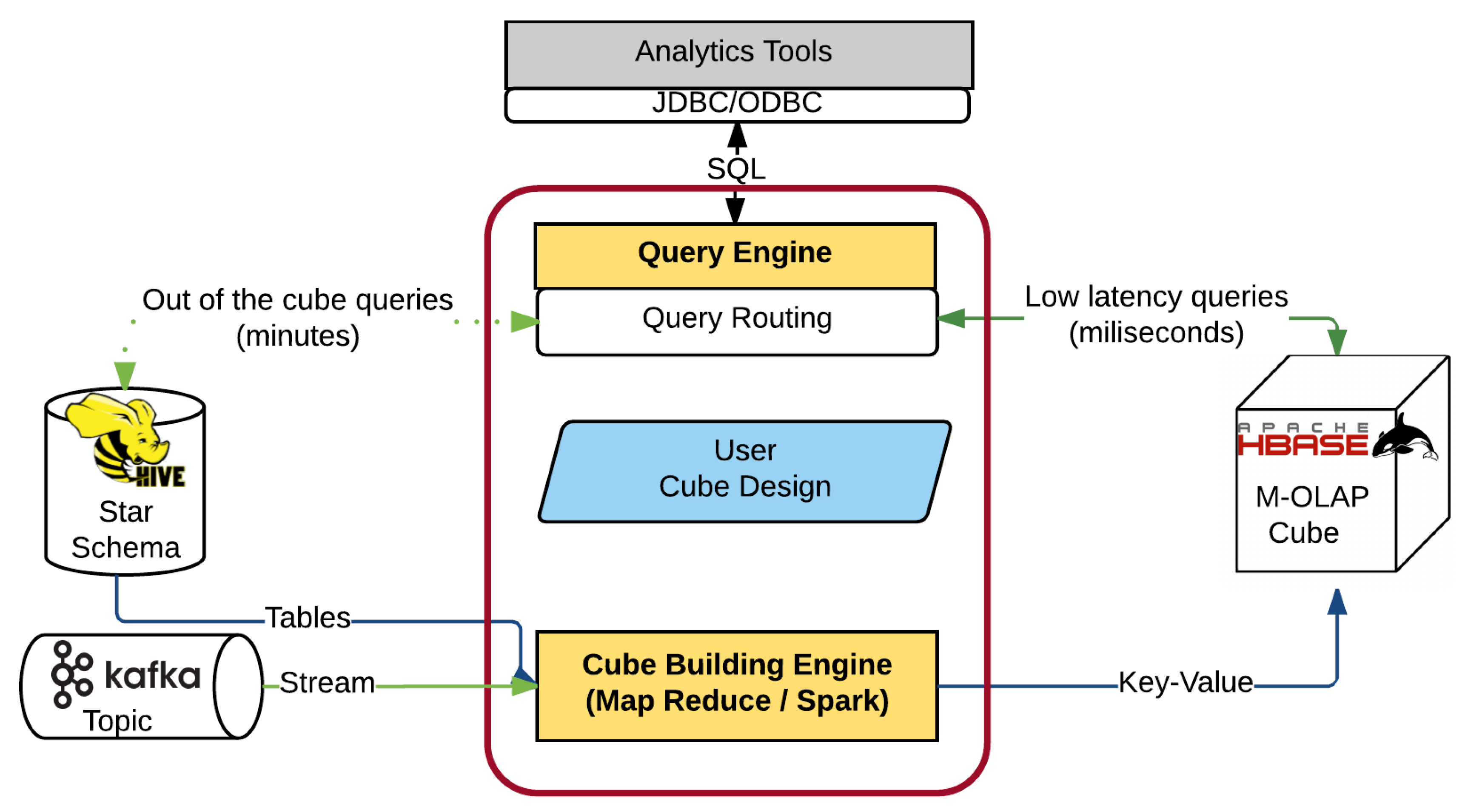
For designing the OLAP cube, Apache Kylin provides a Web UI with step based design. However, despite this aid, designing an OLAP cube with Kylin is not a trivial task. It requires very advanced knowledge of the underlying Hadoop technologies which are part of the Kylin architecture as shown in Figure 2. An example of this required knowledge, is that the user must choose between the two cube building engines that Kylin supports, Map Reduce or Spark, and also provide their configuration. Although Spark is faster than Map Reduce, it is not always recommended or even possible to make use of Spark, since its use is limited to the available RAM memory in the nodes of the cluster. Therefore, Spark could lead to Out Of Memory (OOM) errors that prevent building the OLAP cube successfully, while Map Reduce is a more reliable but slower option. Moreover, the use of the default configuration for the chosen engine is not recommended if we want to take advantage of the full power of the system.

To define the OLAP cube, Kylin can use as data source (i), a Data Warehouse (DW) stored on Hive [21] for batch applications, or (ii), a Kafka topic for real-time OLAP applications. Then the user has to define a cube design including facts, dimensions and their mapping with the data sources along with others parameters, such as dimensions optimizations, algorithm selection or the cube engine used. Using this metadata, the cube building process takes advantage of the distributed processing of Map Reduce [22] or Spark [23]. As a result of this process, an OLAP cube with the aggregated data are generated and stored on Hbase [24]. At this moment, data users can perform analytic queries over the OLAP cube using the Standard Query Languaje (SQL).

As Kylin generates the OLAP cube using a design provided by the user, a wrong design alters significantly several metrics such as the identified for our proposed benchmark in Section 3.1. The design decisions affect the most the goals we have previously identified are those related with dimensions, i.e., contexts of analysis. This is due to Kylin Cube implementation is based on the applications of data pre-aggregation techniques, thus suffering of Curse of Dimensionality issue [25]: The more dimensions, the greater will be the number of combinations between dimensions for which pre-aggregation has to be generated. While this pre-aggregation usually improves query latency over the generated cube, cube building success, time, and cube size metrics are heavily affected. Moreover, a very big cube size could affect the time needed to scan the HBase table, thus increasing query latency. In order to minimize Curse of Dimensionality effects, Kylin implements design techniques that can reduce the number of combinations between dimensions. These design techniques can be grouped in (i), Dimension Types, and (ii), Aggregation Groups.

The Dimension Type determines if the dimension data will be pre-aggregated with other dimensions and facts on building process, otherwise dimension aggregations will be calculated at query time. Kylin supports two dimensions types:

• Normal: A dimension that will be combinated with the other “Normal” dimensions and facts in order to generate data pre-aggregation. These dimensions fully contribute to the Curse of Dimensionality. For example, the measure Credits Approved, combined with the Degree (Computer Science, Maths) and Academic Year (2016, 2017) dimensions, will be pre-aggregated and stored on the OLAP cube for the combinations (Computer Science, 2016), (Computer Science, 2017), (Maths, 2016), (Maths,2017). This will reduce the aggregation needed during query execution time, thus reducing query latency. However, “Normal” dimensions must be defined carefully, as they lead to a combinatorial explosion between dimensions.
• Derived: Often dimensions are stored in tables separated from fact table, as in Star or Snowflake schemas [1]. In these cases, the dimension table columns needed to determine the relationship between this table and the fact table are called Surrogate Keys (SK) [1] and Kylin manage them as “Normal” dimensions by default. However, the remaining columns of a dimension table can be defined as “Normal” or “Derived” dimensions. If we define a dimension column as “Derived”, this dimension is not used for pre-aggregation, thus it has no effects on Curse of Dimensionality. These dimensions will be obtained from the SK of the dimension table and aggregated with other dimensions and facts during query execution time, therefore increasing query latency. However, in what degree a “Derived” dimension could impacts query latency, depends of the cardinality relationship between SK and its “Derived” dimension column, e.g., the cardinality relationship between SUBJECT_ID (SK dimension) and SUBJECT_DES (subject description) is 1 to 1, thus in execution time only is required mapping between these values, due to data are aggregated at the same level in both dimensions. However, if we define SUBJECT_TYPE as “Derived”, where the cardinality relationship with SUBJECT_ID is higher (1/16), more computation for data aggregation will be required during execution time.

In some scenarios, we have a lot “Normal” dimensions, due to (i) the presence of many different dimensions tables, having each one at least one SK treated as a “Normal” dimension, or (ii) many dimension columns with a high cardinality relationship with SK columns, thus we prefer define it as “Normal” dimensions to avoid a high computation requirements during execution time. For these scenarios with many “Normal” dimensions, Kylin provides another optimization called Aggregation Groups. This optimization allows to group “Normal” dimensions that will be pre-aggregated together, enabling cube designers to apply one the following three powerful optimizations to reduce combinations between “Normal” dimensions included on this Aggregation Group:

• Mandatory Dimensions: If a “Normal” dimension is defined as “Mandatory”, all the combinations and pre-aggregations without this dimensions are pruned, e.g., if we define Student, Subject and Academic Year as “Normal” dimensions and also we mark Student as Mandatory, all the combinations between these three dimensions will include the Student dimension.
• Dimension Hierarchies: We can define a hierarchical relationship for a group of “Normal” dimensions. Then only combinations and pre-aggregation for these dimensions in defined hierarchical order are computed during cube building, e.g., we can define the hierarchy SUBJECT_TYPE_ID→ SUBJECT_ID. This means that only the combinations (SUBJECT_TYPE_ID) and (SUBJECT_TYPE_ID, SUBJECT_ID) will be computed during cube building.
• Joint Dimensions: Sometimes we find dimensions that are queried together very often. E.g., Id and description columns are usually queried together, such as SUBJECT_ID and SUBJECT_DES in our data source, however Kylin considers them as two separated dimensions. In this case, we can define a Joint group that includes these two dimensions. Therefore, these dimensions will appear together in all possible combinations between the joint group and remaining dimensions.

Therefore “Derived” Dimensions and Aggregation Groups are powerful tools to reduce Curse of Dimensionality effects. Considering these optimizations and the complete architecture of Kylin, we summarize in the following the design steps and principles to be applied for the OLAP cube implementation:

• Source system selection: If batch processing is required, we recommend using Apache Hive due to its proved capabilities to store and maintain analytical data models for Big Data scenarios. In case of a real-time scenario, we recommend using Kafka.
• OLAP cube definition: First the user must identify the tables and the relationship between them over the data model stored in the source system chosen. Secondly, to reduce the effects of the dimensionality curse [25], it is very important to determine the optimal type for each dimension column. Finally, for those dimensions defined as “Normal”, we have to create one or more aggregation groups and apply to them the possible optimizations allowed. To this end, we recommend conducting a previous study of end-users querying patterns, to achieve a trade-off between pre-aggregation stored in the OLAP cube and the aggregation required during query execution time. Therefore, for our benchmark implementation, we have to study the set of 30 SQL queries proposed to identify such querying patterns.

3.3.2. Benchmark Implementation

In order to effectively implement our proposed benchmark, we chose Apache Kylin [2,3] Big Data OLAP approach, due its power to cope with up to tens of billions of rows fact table, ultra high cardinality dimensions and support for both batch and real-time OLAP scenarios. Moreover, using the previously stated design principles for Kylin cube design, in this section we propose eight different OLAP cube designs using as a data source the academic data model. Then, we use our proposed approach to benchmark these eight cube designs. We analyze the results obtained in order to extract useful insights that help us to improve the OLAP cube design processes for Apache Kylin.

These eight OLAP cube designs proposed are shown in

Table 4. Cube Designs for Benchmark Execution.

Design	Total Normal Dim.	Defined Normal Dim.	Max Sk Rel Derived *	Derived Dim.	Hierarchies	Mandatory	Joint
D1	12	7	1/1	5	0	0	0
D2	10	5	1/10	7	0	0	0
D3	5	0	1/n	12	0	0	0
D4	12	7	1/1	5	0	0	3 of 2 Dim.
D5	12	7	1/1	5	1 of 2 Dim. (1 UHC) 1 of 3 Dim. (2 HC) 1 of 4 Dim.	0	0
D6	12	7	1/1	5	2 of 2 Dim. (1 UHC) 1 of 4 Dim.	1 Dim. (HC)	0
D7	11	6	1/10	7	1 of 2 Dim. (1 UHC) 1 of 3 Dim. (2 HC) 1 of 4 Dim.	0	0
D8	10	5	1/10	7	1 of 2 Dim. (1 UHC) 1 of 3 Dim. (2 HC) 1 of 4 Dim.	0	0

* Maximum cardinality of all pairs (SK Dimension, Derived Dimension), understanding cardinality as the relationship between between an SK dimension and the dimension derived from this SK.

. All of them cover all the analytic model described on Section 3.2, each with design 5 dimension tables. This means each one has five SK columns that are treated by Kylin as Normal Dimensions, as we explained in Section 3.3.1. However, from these SK columns, we can define the remaining columns as “Derived” or as “Normal” dimensions. Moreover, we have identified the cardinality relationship between the SK dimension column and the remaining dimension columns, as one parameter to control the effects of defining “Derived” dimensions. In order to test the trade-off between defining more or less dimension as Derived, the designs D1, D2 y D3 has different number of Normal and Derived dimensions according to the value of cardinality between SK and Normals dimensions proposed (Max Sk Rel Derived): 1/1, 1/10 and 1/n (all as “Derived”).

In designs D4 to D8, we aim to evaluate the use of the Aggregations Groups optimizations. Thus, we define one aggregation group with different subgroups of Hierarchies, Mandatory and Joint dimensions. Using design D1 (Max SK Rel = 1/1) as a base, we defined D4, D5 and D6. In D4 we define three joint groups of two dimensions such as (SUBJECT_TYPE_ID, SUBJECT_TYPE_DES) due to description columns are very often queried together with ID columns. Design D5 is intended to evaluate the use of Hierarchies of dimensions in Aggregation Groups. Therefore, we defined three hierarchies, one of them over Student (UHC) dimension, e.g., we defined the hierarchy ID_NUMBER_SUB3→ ID_NUMBER where ID_NUMBER_SUB3 are the three first characters of an Student ID_NUMBER, thus ID_NUMBER_SUB3 can be used to resume data stored by the dimension ID_NUMBER. Then, in order to test Mandatory optimizations, in D6 we defined ID_NUMBER as mandatory, that will reduce query latency for queries that use ID_NUMBER while increasing latency for queries that do not use this dimension.

On the other hand, D7 and D8 OLAP cubes are designed using design D2 as a base. D7 and D8 designs are aimed to evaluate the combination of a balanced definition of “Derived” dimensions (Max SK Rel = 1/10) in conjunction with defining hierarchies described in Table 3 over the remaining “Normal” dimensions. Differences between these designs are about dimension types and hierarchy defined over Student UHC dimension columns. Therefore, D7 and D8 are two alternative design that applies derived dimensions in 1/10 MAX. SK Rel and hierarchies optimization.

As in D3 all not SK dimensions are defined as “Derived”, we cannot apply any of the Aggregation Groups optimizations due to the fact that they are only applicable to “Normal” dimensions.

Finally, in order to test Query Latency and % Queries > 3 s measures, we have used the proposed set of 30 different SQL queries described in Section 3.2. These queries are classified and distributed in the three groups proposed: High Level Aggregation, Drill Down and Drill Down UHC queries.

4. Results

To execute the proposed design we have used Kylin 2.6 installed on a Hadoop cluster. This Hadoop cluster uses Elastic Map Reduce 5.30 (EMR) Hadoop distribution and Amazon AWS cloud infrastructure, composed of four m4.xlarge nodes each one with 8 vCores and 16 GB RAM. We have also installed Kylin on an additional m4.xlarge machine, which makes use of the EMR cluster for cube building (Map Reduce with YARN) and storage (HBase and HDFS). We consider this cluster is enough powerful to cope with the data model and workload described on Section 3.2.

Moreover, we have used Kylin default “By Cube Layer” cube building algorithm and Map Reduce cube engine. Benchmarking Kylin algorithms (there are two) and cube engine (Map Reduce vs. Spark) are out of the scope of this paper, so we fixed it to the standard values.

Benchmarking results are showed in

Table 5. Results of Benchmark Execution.

Design	Success	OOM Errors	OLAP Cube Size (Gb)	Expansion Rate	% of Coverage	Building Time (hours)	Query Latency (AVG seg)	% Queries > 3 seg
D1	Failure	Yes	-	-	-	-	-	-
D2	Success	No	63.07	40.43×	100%	8.59	12.91	51.52%
D3	Success	No	2.31	1.48×	100%	1.38	11.34	42.42%
D4	Success	No	68.07	43.63×	100%	9.10	5.08	24.24%
D5	Success	No	23.39	14.99×	100%	4.26	4.79	24.24%
D6	Success	No	34.29	21.98×	100%	4.43	15.07	57.58%
D7	Success	No	23.31	14.94×	100%	3.76	4.05	21.21%
D8	Success	No	16.55	10.61×	100%	2.85	5.09	30.30%

. Success, OOM Errors, Cube Size and Expansion Rate are benchmark metrics related to cube building process, therefore we used information provided by Kylin and its underlying hadoop tools to fill these values. Over the generated OLAP cube, we benchmarked average query latency in seconds, as a result of executing the above described set of 30 queries. % of queries with latency over 3 s and % of model coverage are also obtained from queries execution results.

Moreover, as a result of queries execution, in Figure 3 we show average query latency in seconds grouped by query type and cube design and, in Figure 4, we show the % of queries resolved in less than 3 s.

5. Discussion

After the execution of our proposed benchmarking, we analyzed the results in order to extract useful insights to improve the OLAP cube design processes for Apache Kylin. Based on these findings, together with the analyzed principles for cube design, we have proposed a guideline to find the optimal cube design for Apache Kylin.

In Table 5, we can see that D1 cube could not be built successfully. The high number of “Normal” dimensions and the non-application of any of the Aggregation Group optimizations makes the number of combinations too high (2¹²) for computing this cube using a Hadoop cluster. This process requires a lot of memory, thus Out of Memory (OOM) errors can take place in this scenario. However, the remaining designs were built successfully, since they only used design D1 as a basis. In order to generate remaining designs over D1, we increased the number of “Derived” dimensions in designs D3, D4, D7, D8, and we applied Aggregation Group optimizations in D4, D5 and D6 cubes.

If we compare designs D3 and D2, we observe the high impact of defining all D3 dimensions columns as “Derived” has on benchmarking variables. The OLAP cube size is just 1.48 times bigger than the DW used as source (described on Section 3.2) while D2 cube size (where only some dimensions are defined as “Derived”) is 40.43 times the DW source size. Moreover, building time is dramatically reduced in D3 compared with D2 time. Surprisingly, although the computation for aggregation needed in query execution by D3 cube is much bigger than for D2 cube, the Query Latency is a little smaller in D3, about 1 s on average. This could be explained due to the huge Size of cube D3, query execution could need a lot of time to scan all the HBase table where the OLAP cube is stored.

Designs D4, D5 and D6 are based on D1 design but applying Aggregation Groups optimizations over “Normal” dimensions. If we compare this three design, we observe D5 has a smaller expansion rate (14.99×) due to the definition of 3 hierarchies over 9 “Normal” dimensions. Moreover this design has the second smallest query latency of all benchmarked designs, and a reasonable building time of 4.26 h. For design D6, we removed 3 dimensions of the hierarchies used in D5, in order to add one mandatory dimension. The query latency is 15.07 s, the highest result of the benchmark, while the rest of variables are a little bigger than D5. Due to the fact that only a little subset of the queries use the mandatory dimension defined in D6 (ID_NUMBER), query latency will be better for these queries and worse for the remaining. Finally, D4 design define two groups of two joint dimensions instead of the three hierarchies defined on D5 and D6 because Kylin currently do not allow to apply Joint and Hierarchy optimizations over the same dimensions. D4 expansion rate and building time are over 50% higher than D5 and D6 cubes, while Query Latency is good and close to the value of D5.

If we perform a further analysis of the query latency, we realize that the design D6 has the worst results in % of queries resolved in less than 3 s. Moreover, D6 obtain the worst results in Drill Down with UHC queries. As we define as a Mandatory Subject dimension, the queries that involves Student UHC dimension and do not include Subject dimensions, require a high computation to resolve the aggregation. This demonstrates the importance of analyze query patterns before to apply Aggregation Groups optimizations and how the execution of the benchmark can help us to realize of this fact.

Designs D7 and D8 are based on the D2 design with more derived dimensions (MAX SK REL = 1/10) than D1 (MAX SK REL = 1/1), but defining three hierarchies for nine “Normal” dimensions like D5 design. The difference between this design is definition of ID_NUMBER as “Normal” dimension in D7 and as “Derived” on D8. The benchmark results shows that D7 design achieves the best average query latency of benchmark execution, just 4.05 s and only 21.21% of the all queries set responded over 3 s. Compared with the other designs this is one of most balanced, achieving an Expansion Rate of 14.94× and 3.76 h of building time. D8 has slightly better results for Expansion Rate and Building Time, however query latency average is over 1 s worse.

We conclude that best balanced designs are D3 and D7. D3 obtains the best values for variables related to cube building and size, especially for cube building time. This process takes less than two hours, thus an acceptable value for a BI OLAP system with a daily window load. However its 11.34 s of query latency is a little high for an OLAP system, where 42.42% of the queries are executed over 3 s. Although, in some BI scenarios the 3.76 h of building time could be high, D7 cube latency is just 4.05 s, with only a 21.21% queries executed over 3 s, thus this design is very suited for OLAP production environments.

The execution of our benchmark has provided us results that demonstrate that to achieve a good OLAP cube design with Kylin we have to: (i) find a trade-off between the number of “Normal” and “Derived” dimensions, i.e., the trade-off between the amount of data pre-aggregated during cube building (thus stored on cube) and the aggregation needed on query execution time, and (ii) define the Aggregation Groups and its optimizations over “Normal” dimensions accordingly to the analytics data model aimed to implement and end-user query patterns. Based on these findings, together with the analyzed principles for cube design, we have proposed the following guideline for the optimal cube design for Apache Kylin:

• Identify query patterns: We must collect the query requirements from existing queries or user requirements. The aim is to identify the following elements among others: Tables, relations between these tables, most used columns, aggregations on columns, columns that are queried together, hierarchical relations or columns used as filters.
• Define the OLAP cube: Using the information collected about querying patterns.
  • Table and column selection: Include only those tables and columns that will be used. If the cube contains too many dimension columns, we should consider create multiples cubes to reduce its complexity.
  • Dimension type selection: We recommend defining as “Normal” only those dimension columns that occur frequently in the identified query patterns and their performance would be low if we defined them as a “Derived” dimensions. Based on our insights, we can establish that this low performance is often given for cardinality ratios greater than 1/10 with respect to the SK column of the dimension table to this column belongs.
  • Aggregation groups definition: We have to group the columns with dimensions defined as “normal” into aggregation groups that respond to query patterns: Columns queried together, with a hierarchical relationship or those used in all queries (e.g., a date column). Declaring these patterns will reduce the effects of the curse of dimensionality problem and therefore reduce the size and building time of the resulting cube.
• Apply the benchmark: Apply our proposed benchmark to evaluate the cube design.
  • Building the OLAP cube: In case the cube cannot be built due to OOM errors, go back to step 2 to review the cube design criteria to generate a new one.
  • Benchmark execution: In case there are no existing queries, we must design a set of SQL queries based on user requirements. Then, execute this query set and measure query latency and coverage of the model.
• Evaluate results and refine cube design: If the implemented cube does not meet the values required for the goals listed in Table 1, return to step 2 to refine the cube design. Even if the requirements are met, in order to find the most optimal cube, we recommend generating and benchmarking one or more alternative cube designs, based on those design decisions that raised some doubts.

Another important point of discussion is the applicability of our proposed benchmark. In addition to the Kylin implementation presented, we consider that the proposed benchmark is also applicable to other Big Data OLAP systems, especially those that support data pre-aggregation such as Apache Druid.

However, since Druid does not support the definition of star or snowflake models, we have to conduct some minor changes to implement on it the proposed data model. Thus, Druid requires the entire data model to be stored in a single table. This can be done by applying a technique known as data denormalization. Similarly, the 30 proposed SQL queries can be adapted to be executed on this single table. Alternatively, we can apply the supported integration [9] between Kylin and Druid. In that case, no adaptation would be required to apply our proposed benchmark.

On the other hand, for the OLAP cube implementation, we will have to apply the specific design principles of Apache Druid [6] for data pre-aggregation such as define segment and query granularities or applying rollup features for the data ingestion process.

Finally, we summarize and highlight the advantages of our proposed benchmark over other existing approaches:

• It not only allows to compare OLAP systems [11,12,13,14] but also allows OLAP cube designers to compare different OLAP cube designs on a chosen Big Data OLAP technology.
• It can be applied to any OLAP system, but it is specially recommended to be applied on Big Data OLAP systems, because it addresses the specific requirements of Big Data scenarios unlike other proposals [12]. Based on the analysis of these specific requirements, we propose a complete set of benchmarking metrics in contrast to other reviewed approaches [15,16,18,19].
• In addition, unlike other benchmark proposals for Big Data systems [14], our benchmark considers the specifics of the systems that allow for data pre-aggregation to support OLAP scenarios. This is the case of Apache Kylin, where no other cases of benchmark application can be found in the literature.
• Finally, based on the insights extracted from results of the benchmark application for Apache Kylin, we have proposed a guideline to help users find the optimal cube design for Apache Kylin.

6. Conclusions and Future Work

In this paper, we have proposed a new benchmark for Big Data OLAP, aimed at benchmarking OLAP cubes designed by taking advantage of data pre-aggregation techniques provided by any of the current Big Data OLAP appoaches [2,3,4,5,6,7,8]. As a result of our research in state-of-the-art technologies, and our experience implementing Big Data OLAP systems, we identified the main goals related to a successful OLAP cube design. In order to create a benchmark from these goals, we translated them into measures, thus being able to quantify their level of satisfaction for each benchmarked cube design.

In order to show the application of our benchmark, we required to create a specific implementation for a particular technology. We chose Apache Kylin [2,3] as our sample Big Data OLAP approach from the range of candidate technologies due to three reasons: (i) its ability to cope with up to tens of billions row-sized fact tables, (ii) the capability to deal with ultra high cardinality dimensions, and (iii) its support for both batch and real-time OLAP scenarios.

Moreover, we have identified the principles for the design of Kylin cubes and then executed our proposed benchmark across eight different Kylin cube designs. Based on the results, we proposed a guideline to aid OLAP cube designers find the most optimal cube designs for their particular scenarios.

Among the design goals proposed, we included OLAP cube building time. However, we must notice that our benchmark focuses only on the cube building time related to the OLAP engine itself. It is not aimed at including into the equation other measures covering the total amount of time taken since data are acquired, such as time required for data transformation, cleaning, etc. Given that a Big Data pipeline is often composed of many processes, all of them can be a limiting factor, and contribute to the overall time required to build the cube. Moreover, since there is a tradition for incremental loads after the first one, our benchmark metrics could be complemented or even combined with other benchmarks aimed at optimizing the Big Data pipeline. This would provide Big Data system designers an overall view of the suitability of their architected solution.

As part of our future work, we are planning on implementing and comparing the results obtained across several Big Data OLAP approaches [2,3,4,5,6,8], such as Druid (standalone or integrated with Kylin) or Clickhouse. On the other hand, we will study the specifics of Big Data cloud services such as Google Big Query [7] or Azure Synapse with the aim to implement our benchmark on these systems. Furthermore, for these cloud approaches, we propose to carry out vertical and horizontal scalability tests to study their effects on the OLAP cube performance.