In Situ Rubber-Wheel Contact on Road Surface Using Ultraviolet-Induced Fluorescence Method

Abstract

This study examines the relationship between rubber-wheel and the contact area on the road surface. Ultraviolet-induced fluorescence microscopy was used to observe and measure the contact parts with pyranine as a dye solution. The high sensitivity to U.V. light makes it easy to distinguish contact and non-contact regions on a very small scale. The experiment was conducted in static and dynamic conditions to identify its influence on the apparent contact area of rubber-wheel and road surface. The in-situ observation of the contact area was captured and recorded using a high-speed digital camera with 1-inch a CMOS (complementary metal oxide semiconductor) sensor. Additionally, the contact area between rubber-wheel and road surface was measured using an analyzing software. The results show differences in static and dynamic contact conditions based on the operating parameters.

1. Introduction

The study of contact mechanics between tire and road surface is a tribological application science in automobile. The science in which friction is produced arises from the contact between rubber tire and road surface in order to transmit the tractional force. Many studies established the effect of road-tire contact interaction on grip performance, rolling resistance, wear, fuel efficiency, and energy loss, which correlates with each other [1,2,3,4,5,6]. Fuel efficiency can be improved by reducing rolling resistance of vehicles. One way to reduce rolling resistance is by optimizing the tractional force between tire and road surface. In order to optimize the tractional force, Ilse evaluated the tire and surfacing contact stresses and depth texture [2]. Bharat and Sidharth also proved in their experiment that contact patch between tire and road affect the rolling resistance of vehicles [3]. Manfred Kluppel has produced a lot of articles related to contact mechanic of rubber material since around two decades ago. In 2008, Gert Heinrich and Manfred Kluppel had reported an article about rubber friction, tread deformation and tire traction in sliding situation [4]. Their experiment intended to contribute data for tire dynamic contact during cornering and braking for vehicles with Anti-Braking System (ABS).

In general, road-tire contact is highly affected by external factors such as the applied load and moving speed of vehicles. In rainy seasons for example, the water on the road surface significantly affects the grip performance of tire rubber. According to the Michelin corporation report, a tire’s grip performance is reduced to 50% on a wet surface when the car runs at 60 km/h. Similarly, the tire grip coefficient, which is considered as 1 on a dry surface, is reduced to 0.6 on a wet surface with 1.5 mm depth of water when the vehicle runs at 60 km/h. The grip coefficient was 0.4 when the vehicle runs at 100 km/h, showing the effect of running speed to tire grip performance of vehicles [7]. According to the Michelin report, the tire grip coefficient is highly influenced by indentation and road surface roughness. It has an undeniable relationship between tire rubber contact area and grip performance. The information regarding the contact area is significant in designing and improving the tire’s performance. Specifically, more information helps design superior tires. This is achieved when the mechanisms of tire-road contact conditions are well-understood. Moreover, a lot of data are related to the contact between tire and road surface in various conditions, including internal and external factors are needed. For that reason, it is essential to observe and analyze the contact condition between tire and road surface in various conditions.

The contact areas of tire and road surface is part of contacted-soft-material, same as rubber seal and wiper. Various approaches have been used to observe the contact condition and measure film thickness of the contacting parts, including optical interferometry [8], Raman spectroscopy [9], fluorescence microscopy [10,11], and some others [12,13]. In 1996, a group study established an experimental technique that provides high-resolution thickness measurement in the horizontal and vertical directions at 1.4 µm, and 0.5 nm, respectively [14]. This technique was called relative optical interference intensity (ROII). Bongaerts et al. [9], conducted an experiment using Raman microscopy to measure fluid film thickness between rotated and pressed polydimethylsiloxane sphere on a quartz flat disc. The results showed that the contact condition varied due to sliding speed. Fowel et al. [10] used fluorescence microscopy on soft materials to identify the central film thickness of the contact area at a different speed.

Fluorescence was first applied to tribology in the 1970s when Ford and a co-worker measured the surface film thickness of rotating cylinders and raceway using various oils [15]. The approach used depended on natural fluorescence in the oil, emitted in the visible range when excited by a mercury lamp. It was improved by replacing the mercury lamp with a He-Cd blue laser beam (441.6 nm), leading to a longer working distance and wide range of practical applications [16]. There have been reports on fluorescence in many studies. This is because it accurately measures the thickness between two surfaces through fluorescence light based on the actual amount of liquid within the gap. A thicker fluorescence fluid solution uses higher intensity of light emitted from the lubricant (fluorescence solution). This happens when using the same amount of excitation energy source and concentration of fluorescence dye. The accuracy and precision of this method depend on the amount of fluorescence liquid, dye solution, and exited sources energy [17,18].

In this study, an apparent contact area experiment was conducted to gain a better understanding of tire rubber contact. A rubber-wheel (same material as tire rubber) and road surface replica were used as contacting parts in static and dynamic conditions. The static test was conducted to provide the information regarding the rubber contact due to the effect of the applied load. The dynamic test was meant to provide rubber contact data due to moving speed dependency. The experiment was simulated under wet surface conditions. The road surface replica was covered with fluorescence liquid, while ultraviolet-induced fluorescence microscopy was used to observe the contact area using pyranine as a dye.

2. Methodology

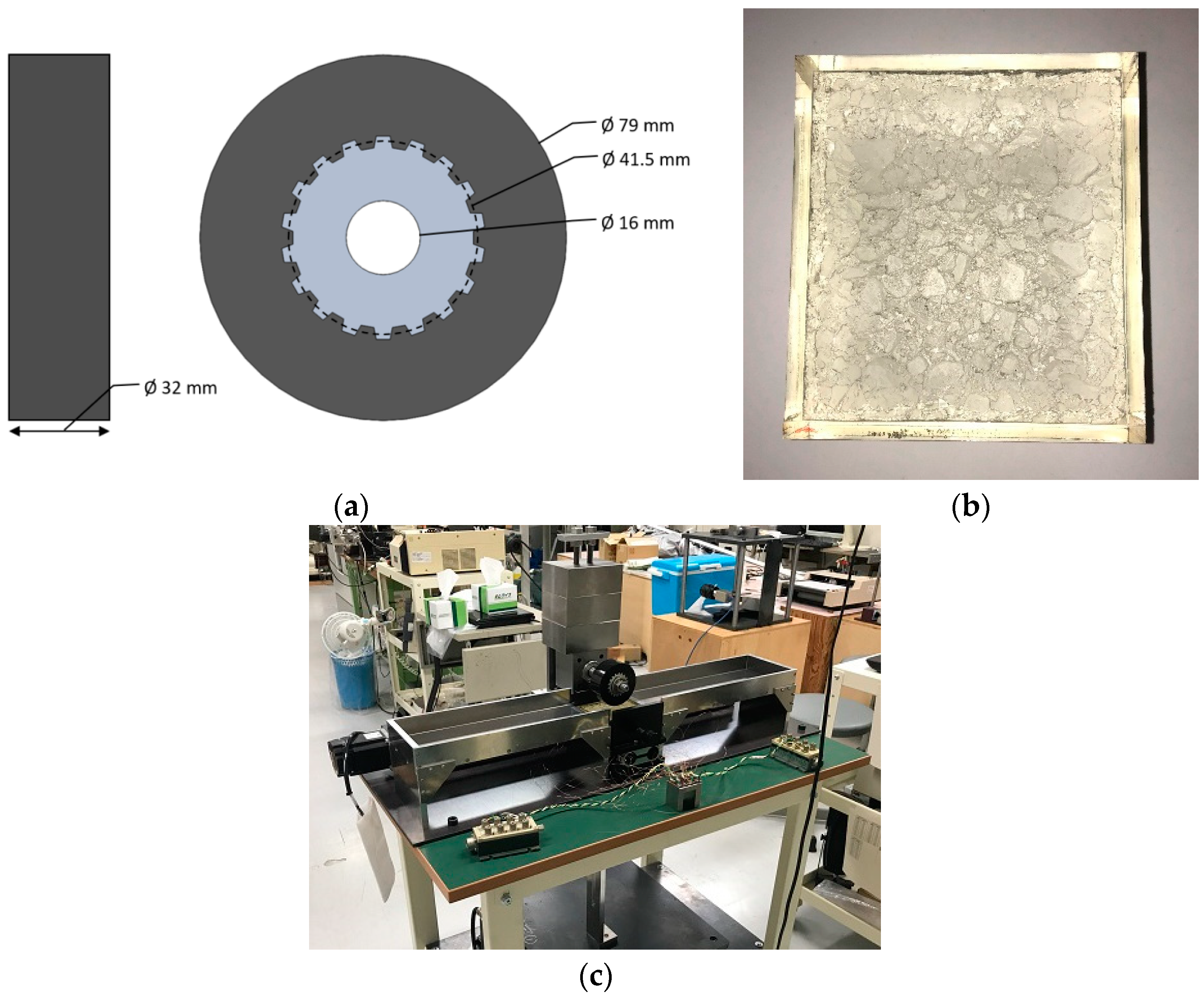
2.1. Experimental Setup

Figure 1 shows the dimensions of the rubber-wheel, road surface replica, and the assembled image of the experimental apparatus for the current study. The contact area was measured using a smooth surface of rubber-wheel and a patterned transparent urethane material copied from the actual road surface. The experiment used macro-rough and micro-rough road surface (based on Michelin report 2001), which has the best friction coefficient in damp and wet conditions [7]. The road surface replica was covered by fluorescence liquid of pyranine solution representing wet conditions in the rainy season. The rubber-wheel was cylindrical, with an outer diameter, inner diameter, and width of 79 mm, 41 mm, and 32 mm, as shown in Figure 1. The inner side of the rubber was fixed on a gear-shaped aluminum with 16 mm inner diameter. The rubber-wheel was connected to a shaft through an aluminum hole for free rotation. Also, the shaft was connected to a linear guide instrument with a vertical loading adjustment and flexible speed for dynamic condition tests. Consequently, the driving force was produced by a linear guide instrument instead of rubber-wheel rotation. Figure 1b shows the contacting part image of road surface replica made of urethane material. This is a rectangular surface of 98 mm × 108 mm in lengths and 37 mm of thickness.

Table 1. Specification of road surface replica.

Specimen	Urethan
Dimensions, mm	98 × 108 × 37
Density, g/cm3	2.51
Poisson’s ratio	0.35
Young modulus, MPa	200

and

Table 2. Specification of rubber-wheel.

Specimen	Tire Rubber
Diameter, mm	ø79
Width, mm	32
Poisson’s ratio	0.49
Young modulus, MPa	2

shows road surface replica and rubber-wheel specifications.

In this apparatus, the contact area was observed using a high-speed digital camera (HAS-U2; DITECT, Ltd., Japan) with 1-inch CMOS sensor, adjustable gain number and image size. The camera produced a maximum of 7500 frames per second (fps) for recording images of high-speed movement. The excitation light source was provided by ultraviolet (U.V.) light with a 365 nm peak of wavelength. The apparatus mechanism differed from the laser-induced fluorescence (LIF), which uses a half or dichroic mirror to reflect the light source perpendicular to the observing surface. The current experiment utilized a ring-shaped U.V. device as a light source for excitation, located beneath the road replica. The dichroic filter and high-speed camera were placed in the middle and below the U.V. light source, respectively. The high-speed camera directly captured the image of contact between rubber-wheel and road surface replica without utilizing a half-mirror or dichroic mirror. Also, the working distance of the high-speed camera and rubber-wheel contact could be modified based on a wide range of the image. The green-dichroic-filter (passing wavelength between 505 nm and 575 nm) was placed on the top of the camera to capture the only green color of fluorescence light for analysis. Hence, the apparatus enabled us to conduct an experiment for in-situ observation and measure a wide range of contact area. The captured images were then recorded to P.C. for further analysis. The detailed outline of the observation system is shown in Figure 2.

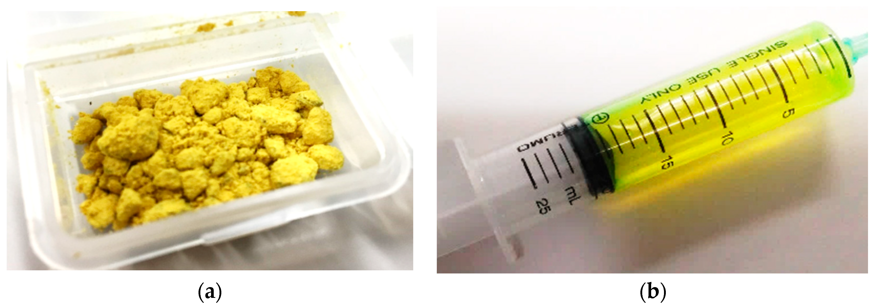
2.2. Pyranine Solution

Pyranine is one of the readily available fluorescence compounds with a chemical composition of C₁₆H₇Na₃O₁₀S₃ and 524.39 g/mol molecular weight. This study used pyranine dye because it has a large gap wavelength between the excitation light source and emitted fluorescence light, making it easy to confirm and differentiate all contact and non-contact regions by observing the pyranine solution in the contacting parts. Moreover, the invisibility of ultraviolet light makes it convenient to observe the contact condition. The pyranine solution was used for various purposes, such as a pH indicator [19] and a tracer agent. Figure 3 shows the image of pyranine dye mixed with distilled water (pyranine solution).

This study used U.V. light with a peak wavelength of 365 nm as an exciting energy source to illuminate pyranine liquid solution (mixed pyranine dye within distilled water). When the U.V. light is absorbed by pyranine solution, it releases green fluorescence light, a spectrum with a peak wavelength of 513 nm. However, the emission of fluorescence intensity depends on dye concentration, amount of liquid, excited source, salt, and P.H. [20,21,22].Therefore, the experiment was performed with the same parameters for the emission to indicate only the existence of fluorescence liquid. This helps differentiate the contact and non-contact areas easily. The selected pyranine solution concentration applied was 3200 mg/L. This is because the highest intensity is emitted for a small amount of pyranine solution.

2.3. Experimental Condition and Procedure

The rubber-wheel contact with road replica was captured using the high-speed digital camera under stationary and dynamic conditions. As shown in

Table 3. Experimental conditions for static contact.

Contact Condition	Applied Load (N)
Static contact	40.2
Static contact	50.0
Static contact	59.8
Static contact	69.7
Static contact	80.4
Static contact	90.3
Static contact	99.1
Static contact	121.6
Static contact	140.3
Static contact	159.9

, the stationary test was conducted by pressing the rubber-wheel with several variant normal loads, ranging from 40.2 N to 159.9 N. As the rubber kept deforming during pressing (called creep deformation), rubber creep experiment was conducted to obtain the selected pressing time in which the creep deformation was minimal to be ignored. Figure 4 shows the deformation of the rubber-wheel contact area caused by 40.2 N load, with over 600 s of pressing time. The result shows that the appropriate pressing time was 300 s, beyond which the deformation of the rubber-wheel contact area was minimal. The same pressing time was used by Satoru et al. when conducting a stationary test to measure the contact area [23]. Therefore, the rubber-wheel contact area of the experiment on the static test was maintained for 300 s before the image was captured. In the stationary contact experiment, the rubber-wheel was removed from the road replica for about 300 s after capturing the contact image. This was to ensure the rubber-wheel returned to its initial condition for the next load test.

The dynamic condition test used a loaded rubber-wheel, running on the top of fluorescence-liquid-covered road surface replica with a constant moving speed of 4, 8, 20, 40, and 80 mm/s. These were 5 different moving speeds, respectively, as one set. Every set of dynamic tests were performed for 3 types of applied loads of 40.2, 60.8, and 80.4 N, respectively. In this study, the speed represented free rotation which is mixed movement of rolling and sliding. The information on the applied load and moving speed in the dynamic test is shown in

Table 4. Experimental conditions for dynamic contact.

Contact Condition	Applied Load (N)	Moving Speed (mm/s)
Dynamic contact		4
Dynamic contact	40.2	8
Dynamic contact	60.8	20
Dynamic contact	80.4	40
Dynamic contact		80

. The apparent contact areas during movement were captured at 100 frames per second (fps) and a shutter speed of 1/200. The detailed information on high-speed camera specifications for every image is shown in

Table 5. Specification of the captured image.

Camera	High-Speed Camera
Field of view, mm	40 × 30
Number of pixels, pixels	1600 × 1200
Frame rate, fps	100
Shutter speed,	1/200

.

The temperature of the dye solution has an impact on fluorescence intensity [24]. Therefore, all experiments were performed in an air-conditioned room with temperature and humidity set at approximately 23 °C, and 65%, respectively. Also, the distilled water used for the pyranine solution came from the same source with constant density and P.H.

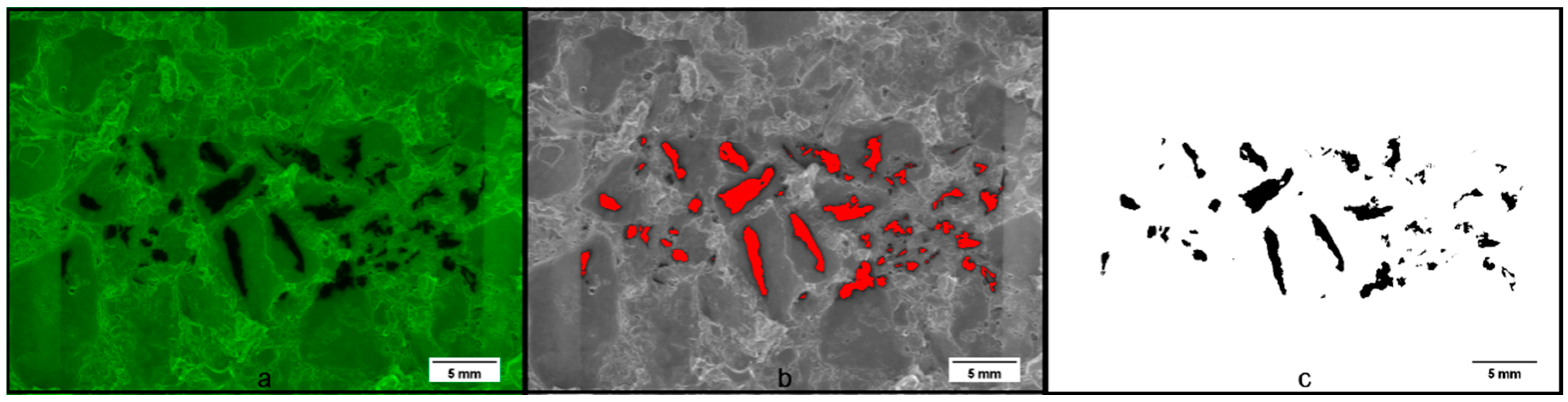
2.4. Apparent Contact Area Determination

As the current study used irregularly patterned road surface replica, the biggest problem was light reflection and scattering, as well as the impurity inside urethane material. Consequently, it was difficult to directly identify the contact region based on fluorescence intensity. There is currently no method to determine the correct boundary of the contact area other than using the thresholding number. According to studies, the Otsu thresholding method is the best in deciding the most appropriate number in image analysis. It was reported that the accuracy of the Otsu thresholding method through an experiment using the Weizmann Segmentation Database was more than 93% [25]. In line with this, the current study used the Otsu thresholding method to determine the boundary for the apparent contact area of rubber-wheel and road surface replica.

Despite its excellency in determining thresholding value, the Otsu method cannot directly be used on rubber-wheel contact on road surface replica. This is because the irregular pattern of the road surface disturbs the calculation of determining thresholding value. In the Otsu thresholding method, all image information is recognized as essential data to be calculated. It cannot be explicitly classified into intended information with many variables on the image. As shown in Figure 5, the binary image based on the Otsu thresholding method for road surface indicates the contact and other areas with no rubber-wheel contact. Therefore, the thresholding value was decided based on rubber-wheel contact on the flat surface of urethane material. The urethane material had the same properties as road surface replica. Figure 6 shows the image of rubber-wheel contact on a flat surface of urethane material and its binary image. The value produced using the Otsu thresholding method was 36. Later, this thresholding value was used to measure the apparent contact area of rubber-wheel and road surface replica. Figure 7 shows the image of rubber-wheel contact on a road surface replica. Also, it shows the binary images of the apparent contact area based on the Otsu thresholding method. The binary image in Figure 7b,c display only the contact area of rubber-wheel and road surface replica. The following experimental data of the contact area between rubber-wheel and road surface replica were measured based on a thresholding value of 36.

3. Results and Discussion

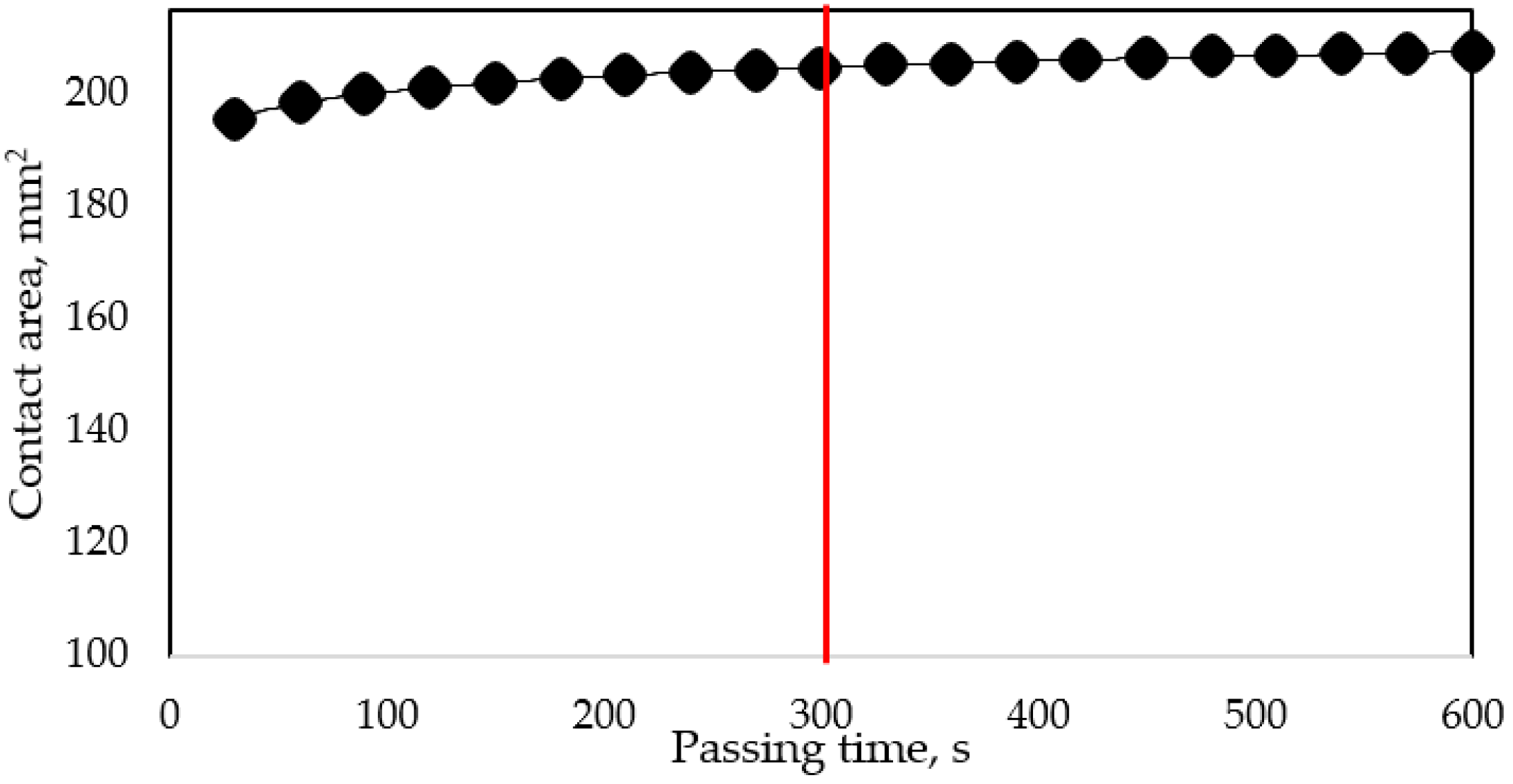
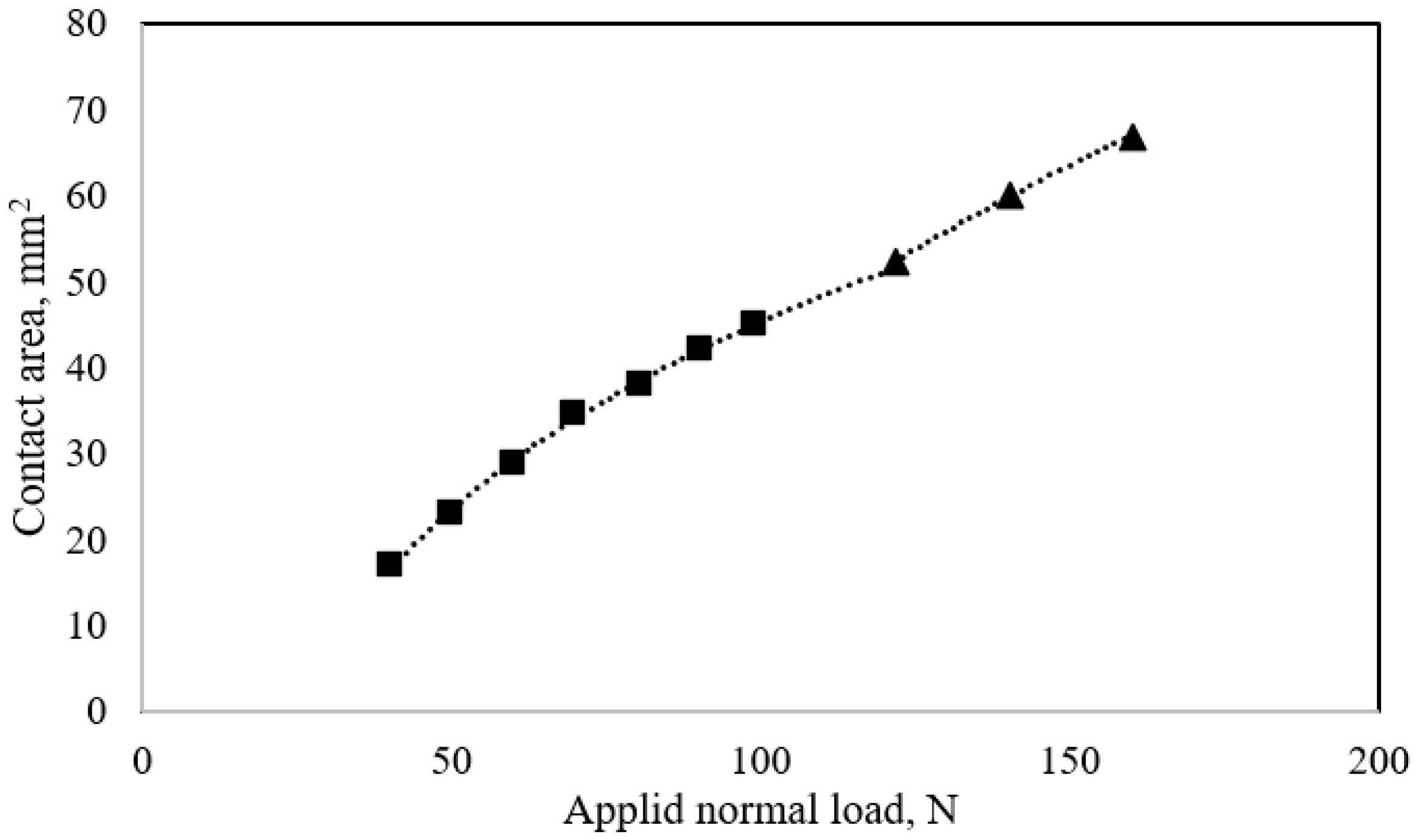
3.1. Contact Area in Static Condition

Tire rubber generates grip (coefficient of friction) caused by the indentation and the molecular adhesion stress mechanisms, respectively. Since rubber-wheel is viscoelastic, it deforms and adapts to the road surface texture when the normal load is applied to the system of the experimental device. Moreover, the contact area is formed through the molecular interaction between rubber-wheel surface and road surface, generating a coefficient of friction [26]. Figure 8 shows the red color binary image of the contact area between the cylindrical rubber-wheel and road surface replica. This represents the 10 selected normal loads of static condition test and the measured rubber-wheel apparent contact area shown in Figure 9. The red color binary was presented in Figure 8 as to make it easy to detect which part of the road surface were in contact with the rubber-wheel. It was easy to distinguish between contact and non-contact areas due to the significant color differences. The red color represented the contact area, while others indicated the non-contact area. However, it was quite challenging to measure the contact area because the loads used were based on the image colors shown in Figure 8. Therefore, the Otsu method was needed to obtain the thresholding boundary value for measuring the contact area of the images. As previously explained, the thresholding value obtained for the contact area was 36. Consequently, the intensity 36 and below was considered as apparent contact region. Similarly, the intensity above 36 was regarded as non-contact region.

Figure 8 shows that the apparent contact area between rubber-wheel and road surface replica was larger because the applied normal load increased. This means that the higher load increases the deformation of the rubber-wheel. Additionally, the rubber-wheel adapts more to the texture of the road surface, forming a larger real contact area. As presented in Figure 9, the contact area increases linearly when the applied normal load increases up to around 70 N. The high resistance within the rubber-wheel on higher applied load deteriorates the expansion of the real contact area, forming a trendline like a logarithmic pattern. The trendline of the graph seems shifted from original pattern when the applied load was 120 N. This formed two different logarithmic trendlines, from 40.2 N to 121.6 N and from 121.6 N, until 159.9 N, respectively. The reason for this was the irregular pattern of the road surface replica, causing some of its new parts to bump with rubber-wheel as applied load increased. However, looking the graph as one whole body, the contact area of rubber-wheel increased proportionally as applied loads increased. This result shows similar tendency with theoretical approach developed by B.N.J. Persson [27].

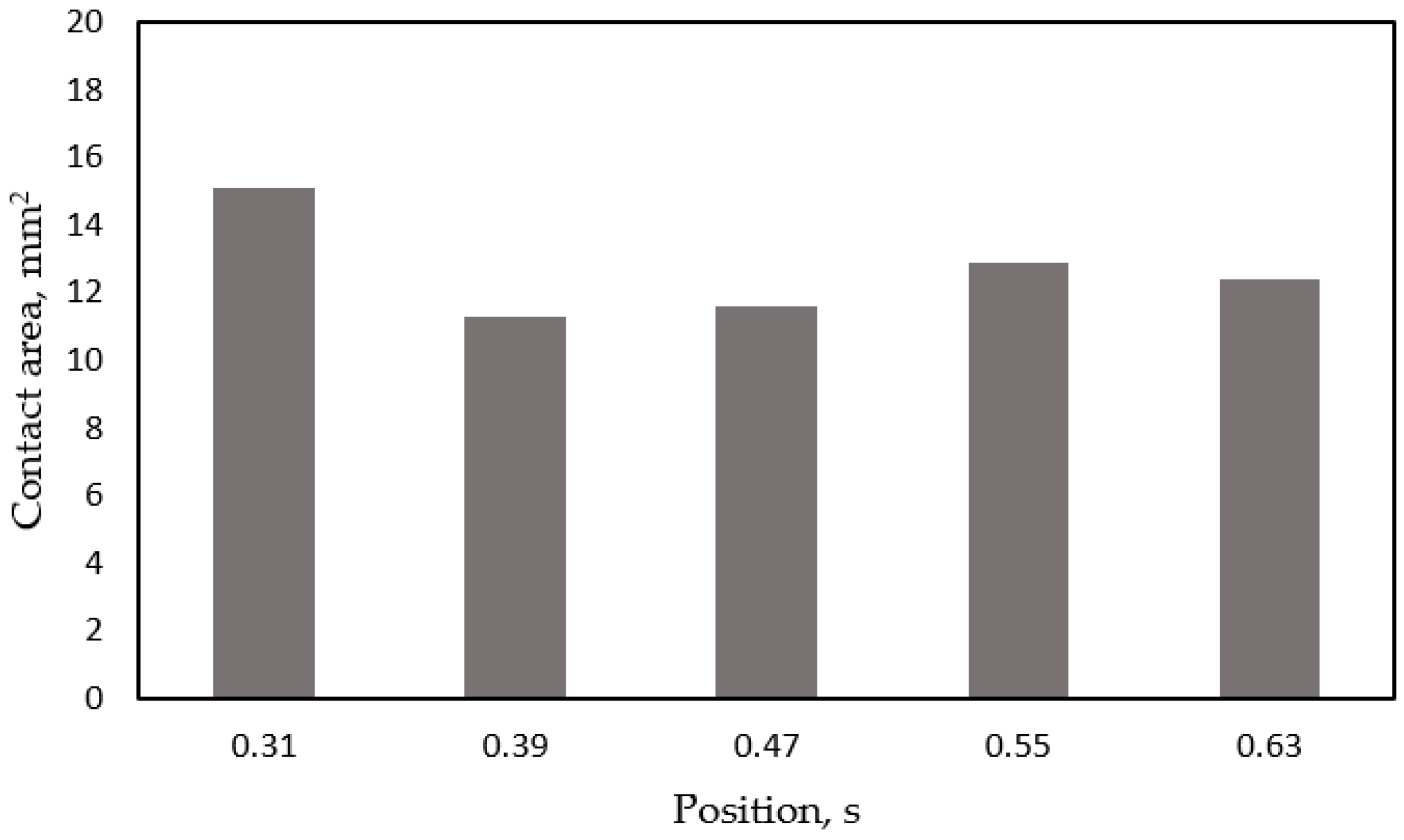
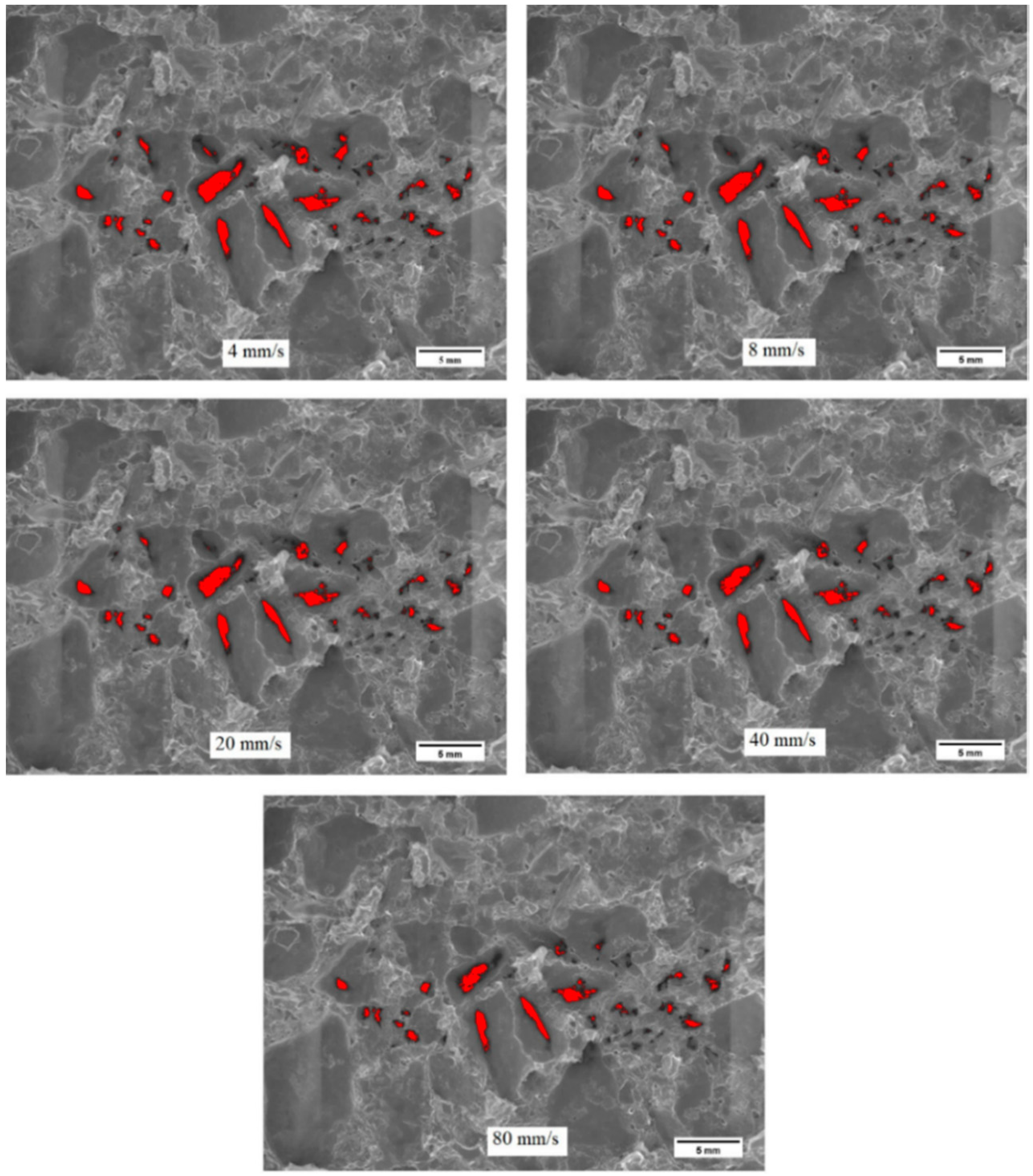
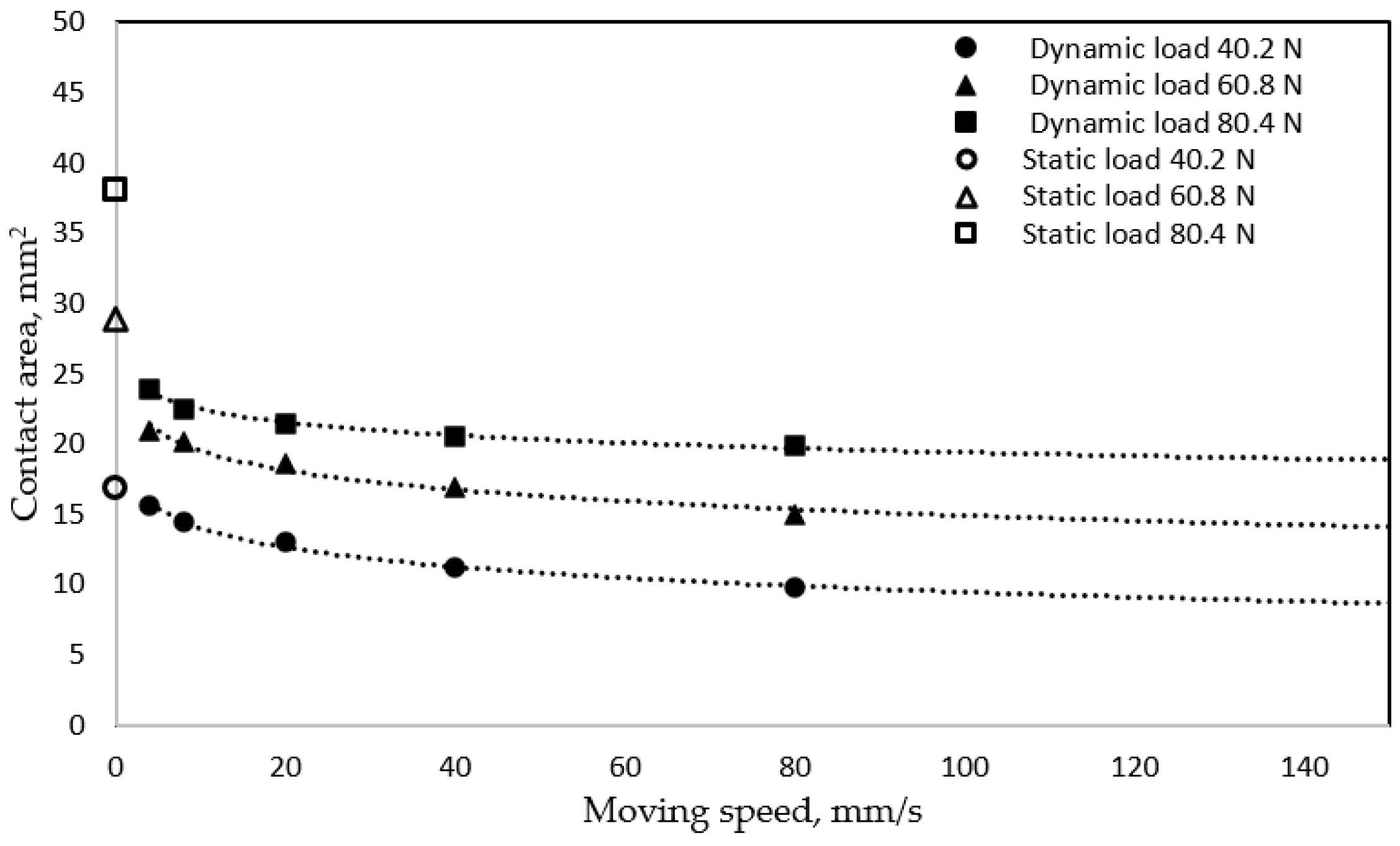
3.2. Contact Area in Dynamic Condition

The dynamic contact images shown in Figure 10 illustrate the condition between a rubber-wheel and road surface replica moving at 40 mm/s under a normal load of 40.2 N. The high-speed camera recorded the moving images along the path using 100 fps. This means it took 0.75 s to cross the camera capture area of 30 mm. Figure 10 only shows 9 out of 75 images, which sufficiently show the movement of rubber-wheel contact from one side to the other. Each position of rubber-wheel contact revealed a divergent contact footprint pattern, displaying different amounts of the real contact area. Figure 11 illustrated the amount of real contact area between rubber-wheel and road surface replica for rubber contact of 0.31–0.63 s. The 5 selected contact images displayed the entire rubber-wheel real contact area. Due to the irregular pattern of the road surface, the real contact area of the rubber-wheel in these images ranged from 11 to 15 mm². It could vary according to surface roughness and pattern.

Figure 12 shows the images of moving speed influences on the contact area between a 40.2 N loaded rubber-wheel and road surface replica in the same position. The images display the contact area of the rubber-wheel that decreased as the moving speed increased. The actual amount of contact area of rubber-wheel is shown in Figure 12. The grip force is produced by the molecular adhesion interaction between rubber-wheel and road surface. Consequently, the bond breaks and forms repeatedly along the movement of rubber-wheel. The stretching adhesion bond gets weaker as the rubber-wheel moves at a certain speed. Therefore, the contact area of a stationary rubber-wheel was always higher than in the dynamic condition. The faster-moving rubber-wheel weakened the adhesion interaction. Similar results were reported by Binshuang Zheng and co-workers in their article titled “Adhesion Characteristic of Tire-Asphalt Pavement Interface Based on a Proposed Tire Hydroplaning Model” [28]. Consequently, the rubber-wheel contact area was smaller as the moving speed increased. These phenomena were present in all the 3 applied loads in the negative logarithmic trendline. The only different thing was that a higher applied load increased the wider contact area. A higher applied load makes the penetration of road surface roughness into the rubber-wheel to be deeper. Consequently, it reaches a wide range of road surfaces. The real contact area of the rubber-wheel observed through fluorescence microscopy widened as the applied load increased.

There are filled marks representing the dynamic condition of the rubber-wheel contact area. Also, unfilled marks are regarded as static conditions of rubber-wheel contact, as shown in Figure 13. The static condition of the contact area was used as a comparison with the dynamic contact. It also helps determine the trendline of rubber contact at a very slow moving-speed. As a result, it can be predicted the reduction of rubber-wheel contact was very significant at a moving speed below 20 mm/s. On the contrary, it reduced slightly to an almost constant line at a moving speed above 20 mm/s. This shows that the contact area of the rubber-wheel is highly affected by the moving speed of vehicles. According to the Micheline report, the grip coefficient of tire reduced as vehicle speed increased. Hence, there is a significant relationship between the contact area and the grip performance of the rubber tire. This was seen when they both decreased as the moving speed increased.

4. Conclusions

An ultraviolet-induced fluorescence technique using a pyranine solution of 3200 mg/l was used to observe the contact area between a cylindrical rubber-wheel and road surface replica in situ. According to the results, the contact area of the rubber-wheel increased with the applied load under static conditions. The contact area on the road surface was significantly affected by the topography of the surface pattern. As long as the rubber-wheel remained on the same part of road surface, the contact area increased in a smooth trendline. However, the trendline shifts when the rubber-wheel touches the protrusions of road surface due to applied load.

In the dynamic condition test, the contact area between the loaded rubber-wheel and road surface reduced as the moving speed increased. In all applied normal loads, it reduced significantly at speeds below 20 mm/s, and then continues to decrease gradually at higher speeds above 20 mm/s. The results showed the same tendency of rubber-wheel contact area and grip performance as a result of the moving speed.

References

1. Winroth, J.; Kropp, W.; Hoever, C.; Höstmad, P. Contact stiffness considerations when simulating tyre/road noise. J. Sound Vib. 2017, 409, 274–286. [Google Scholar] [CrossRef]
2. Steyn, W.J.V.; Ilse, M. Evaluation of Tire/Surfacing/Base Contact Stresses and Texture Depth. Int. J. Transp. Sci. Technol. 2015, 4, 107–118. [Google Scholar] [CrossRef] [Green Version]
3. Das, S.; Redrouthu, B. Tyre Modelling for Rolling Resistance; Chalmers University of Technology: Gothenburg, Sweden, 2014. [Google Scholar]
4. Heinrich, G.; Klüppel, M. Rubber friction, tread deformation and tire traction. Wear 2008, 265, 1052–1060. [Google Scholar] [CrossRef]
5. Heckl, M. Tyre noise generation. Wear 1986, 113, 157–170. [Google Scholar] [CrossRef]
6. Moore, D.F. Friction and wear in rubbers and tyres? Wear 1980, 61, 273–282. [Google Scholar] [CrossRef]
7. Michelin. The Tyre Grip. 2001. Available online: http://www.dimnp.unipi.it/guiggiani-m/Michelin_Tire_Grip.pdf (accessed on 2 September 2020).
8. Marx, N.; Guegan, J.; Spikes, H.A. Elastohydrodynamic film thickness of soft EHL contacts using optical interferometry. Tribol. Int. 2016, 99, 267–277. [Google Scholar] [CrossRef] [Green Version]
9. Bongaerts, J.H.H.; Day, J.P.R.; Marriott, C.; Pudney, P.D.A.; Williamson, A.-M. In situ confocal Raman spectroscopy of lubricants in a soft elastohydrodynamic tribological contact. J. Appl. Phys. 2008, 104, 014913. [Google Scholar] [CrossRef]
10. Fowell, M.; Myant, C.; Spikes, H.; Kadiric, A. A study of lubricant film thickness in compliant contacts of elastomeric seal materials using a laser induced fluorescence technique. Tribol. Int. 2014, 80, 76–89. [Google Scholar] [CrossRef]
11. Myant, C.; Reddyhoff, T.; Spikes, H. Laser-induced fluorescence for film thickness mapping in pure sliding lubricated, compliant, contacts. Tribol. Int. 2010, 43, 1960–1969. [Google Scholar] [CrossRef] [Green Version]
12. Gasni, D.; Ibrahim, M.W.; Dwyer-Joyce, R. Measurements of lubricant film thickness in the iso-viscous elastohydrodynamic regime. Tribol. Int. 2011, 44, 933–944. [Google Scholar] [CrossRef]
13. Poll, G.; Gabelli, A. Formation of Lubricant Film in Rotary Sealing Contacts: Part II—A New Measuring Principle for Lubricant Film Thickness. J. Tribol. 1992, 114, 290–296. [Google Scholar] [CrossRef]
14. Ma, L.; Zhang, C. Discussion on the Technique of Relative Optical Interference Intensity for the Measurement of Lubricant Film Thickness. Tribol. Lett. 2009, 36, 239–245. [Google Scholar] [CrossRef]
15. Smart, A.; Ford, R. Measurement of thin liquid films by a fluorescence technique. Wear 1974, 29, 41–47. [Google Scholar] [CrossRef]
16. Ford, R.A.J.; Foord, C.A. Laser-based fluorescence techniques for measuring thin liquid films. Wear 1978, 51, 289–297. [Google Scholar] [CrossRef]
17. Kedziora, K.M.; Prehn, J.H.M.; Dobrucki, J.; Bernas, T. Method of calibration of a fluorescence microscope for quantitative studies. J. Microsc. 2011, 244, 101–111. [Google Scholar] [CrossRef] [PubMed]
18. Liu, B.; Shen, Y.; Zhang, H.; Tang, Z.; Yuan, X.; Liu, C. Visualization of structured packing with laser induced fluorescence technique: Two-dimensional measurement of liquid concentration distribution. Trans. Tianjin Univ. 2016, 22, 466–472. [Google Scholar] [CrossRef]
19. Avnir, Y.; Barenholz, Y. pH determination by pyranine: Medium-related artifacts and their correction. Anal. Biochem. 2005, 347, 34–41. [Google Scholar] [CrossRef]
20. Zhu, H.; Derksen, R.; Krause, C.; Fox, R.; Brazee, R.; Ozkan, H. Fluorescent Intensity of Dye Solutions under Different pH Conditions. J. ASTM Int. 2005, 2. [Google Scholar] [CrossRef] [Green Version]
21. Santana, J.; Perez, K.R.; Pisco, T.B.; Pavanelli, D.D.; Filho, D.B.; Rezende, D.; Triboni, E.R.; Lima, F.D.C.A.; Magalhães, J.L.; Cuccovia, I.M.; et al. A high sensitive ion pairing probe (the interaction of pyrenetetrasulphonate and methyl viologen): Salt and temperature dependences and applications. J. Lumin 2014, 151, 130–137. [Google Scholar] [CrossRef]
22. Barnadas-Rodríguez, R.; Estelrich, J. Effect of salts on the excited state of pyranine as determined by steady-state fluorescence. J. Photochem. Photobiol. A Chem. 2008, 198, 262–267. [Google Scholar] [CrossRef]
23. Satoru, M.; Fumihiro, I.; Takashi, N. Optical measurements of real contact area and tangential contact stiffness in rough interface between an adheshive soft elastomer and a glass plate. J. Adv. Mech. Design Syst. Manuf. 2015, 9, 1–14. [Google Scholar]
24. Bur, A.J.; Vangel, M.G.; Roth, S. Temperature Dependence of Fluorescent Probes for Applications to Polymer Materials Processing. Appl. Spectrosc. 2002, 56, 174–181. [Google Scholar] [CrossRef]
25. Hidrovo, C.H.; Brau, R.R.; Hart, U.P. Excitation nonlinearities in emission reabsorption laser-induced fluorescence techniques. Appl. Opt. 2004, 43, 894–913. [Google Scholar] [CrossRef] [PubMed]
26. Syafi’i, S.I.; Wahyuningrum, R.T.; Muntasa, A. Segmentation obyek pada citra digital menggunakan metode Otsu thresholding. J. Inform. 2015, 13, 1–8. [Google Scholar]
27. Persson, B.N.J. Elastoplastic contact between randomly rough surfaces. Phys. Rev. Lett. 2001, 87, 116101. [Google Scholar] [CrossRef] [Green Version]
28. Zheng, B.; Huang, X.; Zhang, W.; Zhao, R.; Zhu, S. Adhesion Characteristics of Tire-Asphalt Pavement Interface Based on a Proposed Tire Hydroplaning Model. Adv. Mater. Sci. Eng. 2018, 2018, 1–12. [Google Scholar] [CrossRef] [Green Version]
Figure 1. (a) Rubber-wheel dimensions, (b) Transparent road surface replica (pavement), (c) Experimental setup of ultraviolet-induced fluorescence.
Applsci 10 08804 g001
Figure 2. Outline of Observation system.
Applsci 10 08804 g002
Figure 3. (a) Pyranine substance, (b) Fluorescence solution of pyranine.
Applsci 10 08804 g003
Figure 4. Rubber-wheel deformation due to elapsed time.
Applsci 10 08804 g004
Figure 5. Rubber-wheel contact on the road surface of urethane material under normal load 40.2 N, (a) original image; (b) binary image based on Otsu thresholding.
Applsci 10 08804 g005
Figure 6. Rubber-wheel contact on the flat surface of urethane material under normal load 50 N, (a) original image; (b) binary image based on Otsu thresholding.
Applsci 10 08804 g006
Figure 7. Binarization image of rubber contact on road surface replica under 80,4 N applied load: (a) original image, (b) red binary with road replica background, (c) black and white binary image.
Applsci 10 08804 g007
Figure 8. Fluorescence images of rubber-wheel contact due to applied normal loads.
Applsci 10 08804 g008
Figure 9. Rubber-wheel real contact area due to applied load for static condition.
Applsci 10 08804 g009
Figure 10. The images of rubber-wheel contact while running at moving speed 40 mm/s under 40.2 N of the normal load.
Applsci 10 08804 g010
Figure 11. The images of rubber-wheel real contact area for some position along track path.
Applsci 10 08804 g011
Figure 12. Images of contact area for five different moving speed at the same contact position (images belong to applied load 40.2 N).
Applsci 10 08804 g012
Figure 13. Rubber-wheel real contact area on dynamic condition of three variations applied normal load 40.2 N, 60.8 N, and 80.4 N, respectively.
Applsci 10 08804 g013