Dual-Window Superpixel Data Augmentation for Hyperspectral Image Classification

Abstract

Deep learning (DL) has been shown to obtain superior results for classification tasks in the field of remote sensing hyperspectral imaging. Superpixel-based techniques can be applied to DL, significantly decreasing training and prediction times, but the results are usually far from satisfactory due to overfitting. Data augmentation techniques alleviate the problem by synthetically generating new samples from an existing dataset in order to improve the generalization capabilities of the classification model. In this paper we propose a novel data augmentation framework in the context of superpixel-based DL called dual-window superpixel (DWS). With DWS, data augmentation is performed over patches centered on the superpixels obtained by the application of simple linear iterative clustering (SLIC) superpixel segmentation. DWS is based on dividing the input patches extracted from the superpixels into two regions and independently applying transformations over them. As a result, four different data augmentation techniques are proposed that can be applied to a superpixel-based CNN classification scheme. An extensive comparison in terms of classification accuracy with other data augmentation techniques from the literature using two datasets is also shown. One of the datasets consists of small hyperspectral small scenes commonly found in the literature. The other consists of large multispectral vegetation scenes of river basins. The experimental results show that the proposed approach increases the overall classification accuracy for the selected datasets. In particular, two of the data augmentation techniques introduced, namely, dual-flip and dual-rotate, obtained the best results.

1. Introduction

Hyperspectral images (HSIs) are formed by a grid of pixels, each of them represented by a high-dimensional vector capturing a fraction of the electromagnetic spectrum for that point, sampled at different wavelengths [1]. The high density of the spectral information contained in HSIs, in the order of tens to hundreds of bands for a single scene, increases the ability to identify the materials present in it. This characteristic makes HSIs popular candidates for supervised classification in the field of remote sensing [2].

Deep learning (DL) models have been introduced in the last few years for HSI classification tasks [3,4,5,6] with promising results. Convolutional neural networks (CNNs) [7] in particular, have been successfully used for solving problems requiring multi-class, multi-label classification involving feature extraction (FE) from images [8]. CNNs operate over small cubes of data called patches instead of relying on spectral information alone. These patches are centered around a pixel of the image and taken from a sliding window of a certain size in order to extract spatial-spectral information. A patch is extracted for every pixel of the image using this procedure.

CNNs generally require large amounts of training samples in order to prevent overfitting. Data augmentation is a technique that synthetically generates new samples by applying a set of domain-specific transformations over the original input dataset to improve the generalization capabilities of a classification model. Several data augmentation techniques applicable to HSIs have been proposed, most of which are based on geometric transformations commonly used for image recognition tasks [9]. More recently, [10,11] described hyperspectral data augmentation techniques where pixels are grouped in blocks and different block pairs are used as the input to a CNN. In [12], samples in the original dataset were shifted along its first principal component or based on the average value in each band. Augmentation based on randomly erasing parts of the input patches has also been proven effective for HSI classification in [13]. Finally, generative adversarial networks have been proposed recently as a data augmentation technique in order to generate new samples mimicking the distribution of the original data [14,15,16].

Segmentation is a preprocessing technique capable of simplifying images, reducing them to meaningful, independent regions of pixels with high intra-region similarity and high inter-region dissimilarity called segments. The simplification makes this technique useful to reduce the complexity of subsequent processing tasks. Examples of the use of superpixels in hyperspectral classification as a way to exploit context information can be found in [17,18,19], and as part of a DL classification scheme in [20,21]. In our proposal, superpixel segmentation [22] is used to reduce the computational cost associated with CNN-based classification. During the training and prediction stages, only a representative subset of pixels from each superpixel of the image is selected, allowing for a significant reduction of the computational cost when compared to the sliding window extraction from pixel-based classification.

In this paper, several augmentation techniques relying on geometric transformations aimed at efficient, superpixel-based DL classification for large images are introduced. The main contributions are:

1.

A data augmentation framework called dual-window superpixel (DWS), based on a combination of superpixel segmentation for patch extraction and geometric transformations is proposed. Patches are divided into two regions and the transformations are applied independently to them. This framework is introduced as part of a CNN classification scheme capable of improving the classification accuracy and significantly reducing the execution time of the classification process.

2.

A number of fast and simple data augmentation techniques based on the DWS data augmentation framework are also proposed.

The rest of the paper is divided into four sections. Section 2 describes DWS, the proposed classification scheme and the derived data augmentation techniques. Section 3 details the experimental setup and lists the results obtained. Section 4 presents the discussion about the experimental results. Finally, Section 5 summarizes the main conclusions.

2. Dual-Window Superpixel Data Augmentation (DWS)

This section describes in detail the DWS data augmentation framework developed as part of this work, and the data augmentation techniques obtained from it. The main stages of DWS are explained below.

2.1. Superpixel-Based Patch Extraction

Usually, in hyperspectral classification using CNNs, a sliding window of a certain size is applied [23] to extract spatial-spectral information from the image I. The contents of this window P, also called patch, are then fed to the network.

The proposed scheme replaces the sliding window with the extraction of patches based on superpixel information in order to reduce the computational cost. These superpixels are obtained by applying simple linear iterative clustering (SLIC) [24], a low-complexity superpixel segmentation method commonly used in computer vision, to the image I. Figure 1 shows the result of applying SLIC to the Salinas hyperspectral scene. Strong adherence of the superpixel boundaries to the edges of the image can be observed.

Figure 2 shows the first stages of DWS, related to the acquisition of the patches, prior to the data augmentation itself. The chosen patch size in this example is $25\times 25\times B$, B being the number of bands in the image I. After the application of SLIC to I, each of the resulting superpixels is considered a sample, and a patch is extracted from its center. This reduces the number of processed patches from $W\times H$, W and H being the spatial dimensions of the image, to a much smaller number of superpixels.

2.2. Patch Subdivision

Augmentation operations are commonly performed on the patch as a whole. The complete patch is flipped, rotated, etc. This paper hypothesizes that, in contrast, applying transformations over independent regions of the patch would produce better results. The patch subdivision operation in Figure 2 depicts the patch subdivision stage proposed in this paper. Patches are divided into two regions according to the distance from the central pixel. In the example, the inner region is set to $15\times 15$ pixels. This subdivision makes it possible to apply transformations to the inner region and outer regions of the patch independently. Any transformation able to operate over a patch of data can be applied, regardless of its nature.

The process of patch extraction and subdivision is shown in more detail in Figure 3. On the left, the borders of the different superpixels obtained after applying SLIC over the image are depicted, along with the central pixel of one of the superpixels. The black square centered on that same pixel represents a patch of the desired dimensions that will be extracted at that location. The patch, shown on the right, is then subdivided into two regions as part of this stage.

2.3. Patch Transformation

Several augmentation techniques are introduced in this paper using the patch subdivision principle described in the previous section in combination with the traditional rotate and flip transformations. They can be divided into techniques with transformations applied to the inner region (prefixed with the term inner) and techniques with transformations applied to both the outer and inner regions independently (prefixed with the term dual).

Figure 4 shows examples of the outputs of all the techniques considered in this paper. None indicates that no data augmentation is applied to the input patch. Random occlusion (RO), as presented in [13], performs selective data erasing. Rotate and flip are the traditional data augmentation techniques where the homonymous operation is applied over the whole patch. In addition to those, the following techniques are proposed:

1.

Inner-Rotate ($4\times$): A set of 90, 180, and 270-degree rotation operations are applied to the inner region only, yielding up to four samples.

2.

Inner-flip ($4\times$): A set of three flip or mirroring operations is applied to the inner region only, yielding up to four samples.

3.

Dual-rotate ($4\times$/$16\times$): A set of 90, 180 and 270-degree rotation operations are applied to the full patch, yielding four samples. Afterward, for each of those four samples, the same operations are applied again to only the inner region, producing up to sixteen samples per input patch.

4.

Dual-flip ($4\times$/$16\times$): A set of three flip or mirroring operations is applied to the full patch, yielding four samples. Afterward, for each of those samples, the same operations are applied again to only the inner region, producing up to sixteen samples per input patch.

The dual-flip $16\times$ technique is illustrated in Figure 5. The arrows next to the patches indicate flip transformations performed on certain axes. Long arrows each represent a flip applied to the outer patch, whereas small arrows each represent the same operation applied to the inner region. During dual-flip $16\times$ patch transformation, the following operations take place: first, flip transformations over the horizontal axis, vertical axis and a combination of both are applied to the full patch producing patches 1, 5, 9 and 13. Next, for each of the outputs from that step, the same flip transformations are applied only to the inner region (row of transformations at the bottom of the figure).

3. Results

This section contains information about the experimental conditions, datasets used in the experiments and parameter selection. Lastly, the classification results obtained are presented.

3.1. Experimental Conditions

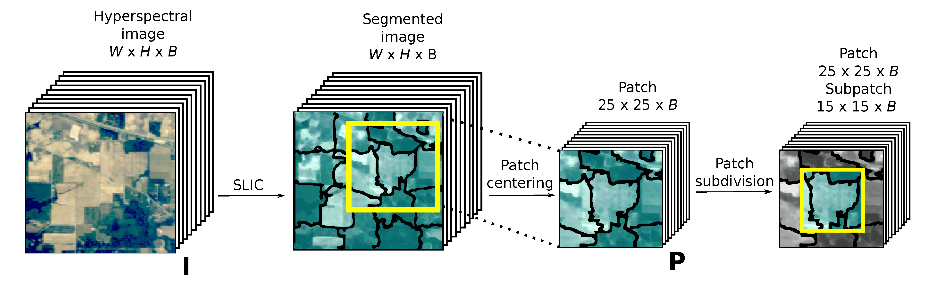
All the experiments were run using the classification scheme and network architecture described in Figure 6. The figure shows, on the left, a patch extracted from the HSI. The black boundaries represent the superpixel edges. The extraction process is explained in Section 2.1. The data augmentation technique of choice was then applied to the patch. The data augmentation techniques based on DWS are explained in Section 2.3. The patches resulting from this data augmentation process were then fed to the CNN.

The network consists of two blocks of 2D-convolutional layers coupled with 2D-max-pooling layers, and two dense layers. With the aim of reducing overfitting, two dropout layers were added to the network, both of them using an aggressive dropout ratio of 0.5.

Table 1. Neural network architecture.

#	Type	Output Shape	Activation	Filter Size	Stride	Padding
1	2D-Convolutional	$25\times 25\times 128$	ELU	$1\times 1$	$1\times 1$	None
2	2D-MaxPooling	$12\times 12\times 128$	-	$2\times 2$	$2\times 2$	None
3	2D-Convolutional	$10\times 10\times 256$	ELU	$3\times 3$	$1\times 1$	None
4	2D-MaxPooling	$5\times 5\times 256$	-	$2\times 2$	$2\times 2$	None
5	Dropout	$5\times 5\times 256$	-	-	-	-
6	Flatten	$1\times 6400$	-	-	-	-
7	Dense	$1\times 256$	ELU	-	-	-
8	Dropout	$1\times 256$	-	-	-	-
9	Dense	$1\times C$	Softmax	-	-	-

details the parameters for each layer. ELU activations were used for all layers due to the advantages this function has over others such as the ReLU family. Namely, ELU provides more robust training and faster learning rates [25]. All trainings were run for 112 epochs using a NADAM [26] optimizer with $\mathrm{learning}\_\mathrm{rate}=0.0001$, ${\beta }_1=0.9$, ${\beta }_2=0.999$, $ϵ=1\times {10}^{-7}$.

In the experiments, data augmentation was performed online for the first epoch and then cached for the rest of the training. The techniques considered are a set of commonly used data augmentation techniques from the literature and the four proposals introduced as part of this work. In the first group we have: rotate, the standard 90 degree rotation applied four times; flip, the standard flip over both axes of the image; PVS(+/−) or pixel-value shift augmentation, where pixel values of the input image are shifted relative to the average band [12]; and random occlusion, which removes rectangular regions of the patch on up to 50% of the input patches in a batch [13]. The new proposals to be studied include inner-rotate, inner-flip, dual-rotate and dual-flip, as described in Section 2.3. The results are compared in terms of classification accuracy after the application of the different data augmentation techniques.

All the tests were run on a 6-core Intel i5 8400 CPU at 2.80 GHz and 48 GB of RAM, and an NVIDIA GeForce GTX 1060 with 6 GB. All experiments were run under Ubuntu Linux 16.04 64-bits, Docker 19.03.5, Python 3.6.7, Tensorflow 2.0.0 and CUDA toolkit 10.0. All the training instances were performed on Tensorflow with GPU support enabled, using single-precision arithmetic.

3.2. Datasets

This section describes the characteristics, including the compositions of the disjoint training and testing sets, of the six scenes used to evaluate the performance of the proposed data augmentation techniques. Three widely available hyperspectral scenes [27] from the literature (standard dataset, from now onwards) and four large multispectral images from river basins belonging to the the Galicia dataset [28] were considered. All the images of the Galicia dataset were captured at an altitude of 120 m by a UAV mounting a MicaSense RedEdge multispectral camera [29]. Its spatial resolution is 0.082 m/pixel and it covers a spectral range from 475 to 840 nm. Figure 7 and Figure 8 display the false color composite and reference data for the scenes of the standard and Galicia datasets, respectively.

More specifically, the Salinas Valley, Pavia University and Pavia Centre scenes from the standard dataset along with the River Oitavén, Creek Ermidas, Eiras Dam and River Mestas scenes from the Galicia dataset were selected for the experiments. The detailed descriptions of the scenes are as follows:

• Salinas valley (Salinas): Mixed vegetation scene in California. It was obtained by the NASA AVIRIS sensor with a spatial resolution of 3.7 m/pixel, covering a spectral range from 400 to 2500 nm. The image is $512\times 217$ pixels and has 220 spectral bands. The reference information contains sixteen classes. The scene is located at 3639${}^{\prime }$33.8${}^{″}$ N 12139${}^{\prime }$58.7${}^{″}$ W.
• Pavia University (PaviaU): Urban scene acquired by the ROSIS-03 sensor over the city of Pavia, Italy. Its spatial resolution is 2.6 m/pixel and covers a spectral range from 430 to 860 nm. The image is $610\times 340$ pixels and has 103 spectral bands. The ground truth contains nine classes. The scene is located at 4512${}^{\prime }$09.2${}^{″}$ N 908${}^{\prime }$08.6${}^{″}$ E.
• Pavia Centre (PaviaC): Urban scene acquired by the ROSIS-03 sensor over the city of Pavia, Italy. Its spatial resolution is 2.6 m/pixel and covers a spectral range from 430 to 860 nm. The image is $1096\times 715$ pixels and has 103 spectral bands. The ground truth contains nine classes. The scene is located at 4511${}^{\prime }$12.7${}^{″}$ N 908${}^{\prime }$48.7${}^{″}$ E.
• River Oitavén (Oitaven): Multispectral vegetation scene of the Oitaven river from Pontevedra, Spain. The image is $6689\times 6722$ pixels and has 5 bands. The scene is located at 4222${}^{\prime }$15.3${}^{″}$ N 825${}^{\prime }$47.4${}^{″}$ W.
• Creek Ermidas (Ermidas): Multispectral vegetation scene showing the point where Creek Ermidas and River Oitavén meet, from Pontevedra, Spain. The image is 11,924 × 18,972 pixels and has 5 bands. The scene is located at 4222${}^{\prime }$51.9${}^{″}$ N 824${}^{\prime }$53.5${}^{″}$ W.
• Eiras Dam (Eiras): Multispectral vegetation scene showing the reservoir that supplies running water to the town of Vigo from Pontevedra, Spain. The image is 5176 × 18,224 pixels and has 5 bands. The scene is located at 4220${}^{\prime }$46.5${}^{″}$ N 830${}^{\prime }$10.5${}^{″}$ W.
• River Mestas (Mestas): Multispectral vegetation scene showing the River Mestas from Pontevedra, Spain. The image is $4915\times 9040$ pixels and has 5 bands. The scene is located at 4338${}^{\prime }$29.8${}^{″}$ N 758${}^{\prime }$42.2${}^{″}$ W.

Table 2 and

Table 3. Oitaven, Ermidas, Eiras and Mestas scenes. Color codes for the classes and number of samples in the training and testing sets used for superpixel-based classification. The ”-” symbol denotes the absence of samples for the specified class.

	Oitaven					Ermidas
		Total					Total
#	Classes	Spp.	Pixels	Train	Test	Classes	Spp.	Pixels	Train	Test
1	Water	611	309,248	367	120	Water	322	163,930	183	70
2	Oak	3710	1,374,889	2227	739	Oak	1992	804,040	1201	390
3	Tiles	192	78,785	112	48	Tiles	224	138,678	137	33
4	Meadows	4464	2,440,331	2709	863	Meadows	5901	3,423,506	3550	1142
5	Asphalt	91	43,861	52	14	Asphalt	1632	737,409	976	331
6	Bare Soil	434	113,329	256	92	Bare Soil	388	123,416	253	83
7	Rock	336	79,152	192	72	Rock	859	174,088	522	172
8	Concrete	358	128,022	206	79	Concrete	64	32,866	45	8
9	Endemic veg.	968	458,565	592	197	Endemic veg.	-	-	-	-
10	Eucaliptus	4260	863,698	2553	838	Eucaliptus	4534	1,135,997	2704	926
11	Pines	717	193,884	430	151	Pines	700	184,547	41 3	149
		Eiras					Mestas
		Total					Total
#	Classes	Spp.	Pixels	Train	Test	Classes	Spp.	Pixels	Train	Test
1	Water	1379	734,617	823	278	Water	-	-	-	-
2	Oak	5559	2,067,380	3332	1066	Oak	-	-	-	-
3	Tiles	17	8232	12	2	Tiles	-	-	-	-
4	Meadows	2457	773,964	1476	485	Meadows	8903	4,489,189	5373	1780
5	Asphalt	145	85,209	86	32	Asphalt	-	-	-	-
6	Bare Soil	401	96,935	247	86	Bare Soil	2708	1,051,275	1653	487
7	Rock	1383	144,800	830	286	Rock	-	-	-	-
8	Concrete	85	27,061	56	16	Concrete	-	-	-	-
9	Endemic veg.	-	-	-	-	Endemic veg.	214	80,858	138	40
10	Eucaliptus	31	8451	23	5	Eucaliptus	9329	449,5047	5540	1887
11	Pines	309	95,132	187	70	Pines	-	-	-	-

show the number of samples for each class for all the scenes in all the scenarios considered in this comparison. The scenes from both datasets were used as follows: 60% for training samples, 20% for testing samples and 20% for validation samples for superpixel-based classification. Table 2 also displays the number of samples for pixel-based classification; 20% of the samples were used, again, as the validation set for this scenario. The number of samples was chosen to prevent an excessively high baseline accuracy when no data augmentation technique was used.

Scenes 1 to 3 were segmented using SLIC with a superpixel size of 50 and a compactness parameter of 20, whereas datasets 4, 5, 6 and 7 used a superpixel size of 800 and a compactness parameter of 40. The compactness determines the balance of space and spectral proximity, with higher values favoring space proximity and causing segments to take on a more square shape.

Two augmentation factors of $4\times$ and $16\times$ were considered, and are displayed in the tables next to the name of each data augmentation technique. For every experiment, the following three accuracy measures [30] are reported: overall accuracy (OA), representing the number of overall pixels correctly predicted; average accuracy (AA), the mean of correctly classified pixels per class; and Kappa ($\kappa$), which measures the agreement between pixel predictions across all classes, also taking into account the occurrences attributed to chance [31]. The values shown are the results of 20 Monte Carlo runs for each scenario. All the values were obtained under identical experimental conditions.

3.3. Superpixel-Based Classification

This section contains the experimental results of the proposal for superpixel-based classification, as described in Section 2. A single scenario training the network with the 60% of the labeled superpixels available has been considered. The classification performance was measured at the pixel level, i.e., considering the same label for all the pixels in the same superpixel.

In order to select values for superpixel size and patch size, some tests were run using one image considered as representative of each of the datasets. PaviaC was selected from the standard dataset and Oitaven was chosen as the counterpart from the Galicia dataset. The results were obtained for two scenarios, one where no augmentation was applied, and a second one where the DWS-based dual-flip $16\times$ technique was used in order to improve accuracy. Values for superpixel sizes each represent an average superpixel area used in the SLIC segmentation. Values for patch sizes each represent the size of a side of the square patch used in the CNN classification process. Inner region sizes are 10 pixels smaller than the corresponding outer regions. The relationship between inner and outer size was chosen as a trade-off between the variability introduced by the transformations applied to the data and the relevance of the inner region. Small changes in inner patch size would not significantly alter the results obtained.

Figure 9 and Figure 10 show the overall classification accuracy for the PaviaC and Oitaven images, respectively, as the superpixel area (left) and the patch size (right) vary. In general, we can observe an inverse correlation between superpixel sizes and accuracy of the CNN model. The accuracy without applying data augmentation is correlated with patch size, and bigger patches produce better results for the Oitaven image. The observed effect is smaller in the case of PaviaC. In this last case, the oscillations in the graph are caused by the dispersion of the values across experiments. Finally, results show a very limited increase in accuracy as the size of the patches grows when using the dual-flip augmentation technique.

The patch size selected for the experiments was $25\times 25$ pixels, with an inner region size of $15\times 15$. The complexity of the proposed CNN is low, and as such, increases in patch size have a small impact during training, allowing us to work with larger amounts of data at this stage. In contrast to this, the amount of samples, most especially when augmentation is applied, has a large impact on the speed of the training stage. Due to this, and in order to keep computation times at moderate values, 50 and 800 were selected as the superpixel sizes for the scenes of the standard and Galicia datasets, respectively.

Figure 11, Figure 12, Figure 13 and Figure 14 show the evolution of the training metrics across all the training epochs. It can be seen how the additional data generated by the augmentation methods cause the training process to converge earlier. As a result, significantly steeper curves in both loss and accuracy can be observed.

Table 4 shows the classification results for Salinas, PaviaU and PaviaC. These images were used for comparison purposes due to their prevalence in land-cover classification papers. Nevertheless, scenes of a size this small see limited benefits from a superpixel level classification, as they are low-resolution and contain very small and irregular structures. Dual-rotate $16\times$ obtained the highest OA for Salinas, which contains bigger and more regular structures. The best results for PaviaU and PaviaC scenes were obtained by the flip $4\times$ and rotate $4\times$ techniques.

Table 5. Superpixel-based classification performance (in percent) for Oitaven, Ermidas, Eiras and Mestas scenes using the training and testing sets detailed in Table 3. The best result for each scene is displayed in bold.

	Oitaven			Ermidas
Technique	OA	AA	$\mathbf{\kappa }$	OA	AA	$\mathbf{\kappa }$
None	94.23 ± 0.44	90.46	92.37	97.20 ± 0.38	92.92	96.00
Rotate $4\times$	95.18 ± 0.46	92.40	93.62	97.83 ± 0.27	94.81	96.91
Inner-Rotate $4\times$ *	95.39 ± 0.55	92.22	93.90	98.08 ± 0.29	95.61	97.25
Dual-Rotate $4\times$ *	94.96 ± 0.33	91.45	93.33	97.70 ± 0.16	94.11	96.71
Dual-Rotate $16\times$ *	96.20 ± 0.14	93.76	94.97	98.32 ± 0.11	96.36	97.61
Flip $4\times$	95.21 ± 0.39	92.78	93.67	98.01 ± 0.26	95.49	97.16
Inner-Flip $4\times$ *	95.56 ± 0.20	93.08	94.13	98.12 ± 0.22	95.86	97.31
Dual-Flip $4\times$ *	95.17 ± 0.30	91.78	93.62	97.91 ± 0.26	95.58	97.02
Dual-Flip $16\times$ *	96.19 ± 0.13	93.16	94.97	98.56 ± 0.15	97.00	97.95
PVSA(+/−) $4\times$ [12]	95.32 ± 0.25	91.26	93.81	97.82 ± 0.29	95.06	96.88
PVSA(+/−) $16\times$ [12]	95.75 ± 0.15	92.66	94.39	98.05 ± 0.18	95.35	97.22
Random Occlusion $4\times$ [13]	93.81 ± 0.49	89.18	91.81	97.19 ± 0.30	93.67	95.99
Random Occlusion $16\times$ [13]	95.68 ± 0.22	92.07	94.28	98.08 ± 0.24	96.08	97.26
	Eiras			Mestas
Technique	OA	AA	$\mathbf{\kappa }$	OA	AA	$\mathbf{\kappa }$
None	95.92 ± 0.53	88.22	93.85	91.05 ± 0.21	85.23	84.85
Rotate $4\times$	96.82 ± 0.32	90.99	95.21	90.76 ± 0.41	84.24	84.32
Inner-Rotate $4\times$ *	96.82 ± 0.35	88.19	95.21	91.32 ± 0.18	86.07	85.30
Dual-Rotate $4\times$ *	96.36 ± 0.19	85.63	94.51	91.06 ± 0.13	84.37	84.86
Dual-Rotate $16\times$ *	97.08 ± 0.25	88.37	95.60	91.67 ± 0.10	87.65	85.93
Flip $4\times$	96.92 ± 0.24	89.47	95.36	90.75 ± 0.34	83.62	84.30
Inner-Flip $4\times$ *	96.96 ± 0.17	89.65	95.42	91.27 ± 0.24	86.91	85.24
Dual-Flip $4\times$ *	96.79 ± 0.22	87.15	95.16	91.15 ± 0.21	85.69	85.02
Dual-Flip $16\times$ *	97.13 ± 0.20	88.81	95.67	91.70 ± 0.09	87.51	85.97
PVSA(+/−) $4\times$ [12]	96.35 ± 0.26	85.70	94.49	91.31 ± 0.24	86.89	85.30
PVSA(+/−) $16\times$ [12]	96.36 ± 0.26	86.27	94.49	91.35 ± 0.14	85.32	85.34
Random Occlusion $4\times$ [13]	95.79 ± 0.28	85.13	93.64	90.72 ± 0.19	82.66	84.27
Random Occlusion $16\times$ [13]	96.83 ± 0.20	86.15	95.21	91.47 ± 0.11	86.24	85.54

* Denotes the techniques proposed in this work.

shows the classification results for the large multispectral scenes of the Galicia dataset, namely, Oitaven, Ermidas, Eiras and Mestas. It can be seen that the proposed classification scheme obtained high accuracy across all datasets, even when no data augmentation was applied during training. Among the techniques tested, approaches based on the DWS framework introduced in this work achieved the best results: dual-rotate $16\times$ and dual-flip $16\times$ reached 96.20% and 96.19% OA for Oitaven, respectively. The results for Ermidas, Eiras and Mestas share many similarities, with dual-flip $16\times$ and dual-rotate $16\times$ leading in terms of OA. When a lower data augmentation factor is considered ($4\times$), inner-flip $4\times$ and inner-rotate $4\times$ can be seen systematically obtaining higher OA values than other methods. It can be seen that techniques based on flips tend to perform better than those based on rotations when applied under similar constraints. Figure 15 shows the resulting classification maps for the images of the dataset.

In order to summarize the results,

Table 6. Superpixel-based overall accuracy delta (in percent) per augmentation technique over baseline performance for all the scenes from the standard and Galicia datasets. The best average result for each dataset is displayed in bold. RO denotes random occlusion.

	Rotate	Inner-Rotate	Dual-Rotate		Flip	Inner-Flip	Dual-Flip		PVSA(+/−)		RO
Scene	$4\times$	$4\times$	$4\times$	$16\times$	$4\times$	$4\times$	$4\times$	$16\times$	$4\times$	$16\times$	$4\times$	$16\times$
Salinas	0.16	1.32	−7.63	3.18	1.16	1.8	−6.56	2.69	1.36	2.11	1.36	1.99
PaviaU	3.13	1.57	−0.98	2.11	3.8	2.45	−1.38	1.11	−0.07	0.8	−0.44	1.19
PaviaC	0.93	0.57	−0.92	0.72	0.84	0.36	−0.62	0.82	0.35	0.59	0.31	0.38
Average	1.41	1.16	−3.18	2.01	1.93	1.54	−2.85	1.54	0.55	1.17	0.41	1.19
Oitaven	0.95	1.16	0.72	1.97	0.98	1.33	0.94	1.96	1.09	1.52	−0.42	1.45
Ermidas	0.63	0.88	0.5	1.12	0.81	0.92	0.71	1.37	0.62	0.85	−0.01	0.88
Eiras	0.9	0.9	0.44	1.16	1	1.04	0.88	1.21	0.43	0.44	−0.13	0.91
Mestas	−0.29	0.27	0.01	0.62	−0.3	0.22	0.1	0.65	0.26	0.3	−0.33	0.42
Average	0.83	0.98	0.55	1.42	0.93	1.09	0.84	1.51	0.71	0.94	−0.19	1.08

displays the performance differences between the baseline performance and each of the augmentation techniques. The results for the standard dataset show dual-rotate $16\times$ was the best performing method overall, followed by flip $4\times$. For the Galicia dataset, dual-flip $16\times$ and dual-rotate $16\times$ obtained the highest increase in OA, with 1.51% and 1.42%, respectively.

3.4. Pixel-Based Classification

This section contains the experimental results of the proposal for pixel-based classification. This scenario was considered in order to show the performances of the proposed augmentation techniques with a traditional pixel-based classification scheme. The scheme applied was the same one described in Section 2, albeit without the superpixel segmentation step. The patches are centered on pixels using a sliding window approach. Tests were run for the Salinas, PaviaU and PaviaC scenes.

Table 7. Execution times (in seconds) for the classification of the PaviaC scene and for each augmentation technique. Prediction time refers to the computation for the whole image.

	Superpixel-Based			Pixel-Based
Method	Training	Prediction	Total	Training	Prediction	Total
None	76.48	5.09	81.57	31.26	2453.79	2485.05
Rotate $4\times$	339.76	6.01	345.77	137.19	2645.13	2782.32
Inner-Rotate $4\times$ *	325.28	5.88	331.16	130.44	2611.15	2741.59
Dual-Rotate $4\times$ *	328.10	6.54	334.64	135.38	2550.93	2686.31
Dual-Rotate $16\times$ *	1305.47	6.16	1311.63	508.97	2770.77	3279.74
Flip $4\times$	325.65	5.30	330.95	129.62	2525.46	2655.08
Inner-Flip $4\times$ *	327.90	5.35	333.25	132.81	2541.49	2674.30
Dual-Flip $4\times$ *	318.98	6.01	324.99	132.51	2528.27	2660.78
Dual-Flip $16\times$ *	1320.23	7.47	1327.70	505.77	2739.75	3245.52
PVSA(+/−) $4\times$ [12]	329.50	7.62	337.12	133.04	2767.88	2900.92
PVSA(+/−) $16\times$ [12]	1306.37	7.53	1313.90	509.75	2770.44	3280.19
Random Occlusion $4\times$ [13]	325.10	7.98	333.08	127.09	2724.73	2851.82
Random Occlusion $16\times$ [13]	1297.85	7.58	1305.43	510.65	2752.50	3263.15

* Denotes the techniques proposed in this work.

displays the execution times of all the augmentation techniques reviewed in this study for the PaviaC scene. Based on the data obtained, we can observe that the total execution times are significantly higher in the case of pixel-based classification. Training times have a very strong linear correlation with the augmentation factor, and thus, with the number of samples being processed. Prediction times are only dependent on the dimensions of the image, and there is little variation across the different executions. It is worth noting that pixel-based classification is not practical for large images due to the large execution time required. The large number of pixels that need to be predicted, three orders of magnitude higher than the number of training samples, causes prediction times to be significantly higher than training times.

Table 8 summarizes the pixel-based classification results for the Salinas, PaviaU and PaviaC images. It can be seen that dual-flip $16\times$ obtained the highest OA for the Salinas scene; inner-flip $4\times$ yielded the highest OA for PaviaU; and flip $4\times$ was the best performing technique for PaviaC. Methods based on flip operations consistently outperformed rotations in this scenario.

4. Discussion

The literature on multispectral and hyperspectral image augmentation contains a multitude of different data augmentation techniques, most of which are used in combination with pixel-based classification. There is a notable lack of proposals approaching data augmentation in combination with superpixel-based classification schemes. Examples of the use of geometric transforms in pixel-based classification schemes can be seen in [13,32,33]. Attempts to synthesize new samples drawing data from a multivariate normal distribution initialized with the standard deviations of the bands in an HSI can be found in [34]. Reference [15] approaches the generation of synthetic samples to be later used in the training of deep networks through the use of GANs, as does [14]. These generative models are very costly to train and require fine-tuned adjustments of the hyperparameters on a per scene basis. The data augmentation framework proposed in this work leverages the composition of simple transformations that require no parameter tuning in order to achieve robust increases in classification accuracy when used in a superpixel-based classification scheme. This makes the derived methods a convenient replacement for the traditional rotation and flip (mirroring) operations.

Reference [35] already introduced the idea of the division of an input patch into several regions in order to better exploit the spatial information. The paper focuses on the selection and extraction of a number of predefined regions surrounding a pixel of interest that are later fed to several CNNs. More examples of the use of the spatial correlation between pixels in a scene can be found in [10], where the authors define pixel-pair features. During the training phase, sample pairs are fed to a CNN architecture that, once trained, is using during the testing phase to compute the labels of the surrounding samples of the pixel being tested and obtain the final label performing a majority vote of the outputs. A similar approach is taken in [11] with pixel-block pairs (PBPs), where the author further builds upon that idea by adding explicit spatial information to the new PBP features. These proposals try to achieve a goal that is similar, in essence, to what DWS does by using the central pixel of each superpixel in order to extract a patch. By selecting the central pixel, the probability of obtaining data from a region with high homogeneity is maximized, yielding an increase in classification accuracy.

To the best of our knowledge, no systematic comparison of data augmentation techniques focused on superpixel-based classification has been published as of yet in the field of remote sensing. The existing papers focus on pixel-based classification and the datasets usually comprise small, low-resolution scenes. An additional factor that increases the difficulty when trying to compare the results from different proposals arises from the use of different models or network architectures to obtain them, making the comparison of the quality between different techniques a challenging endeavor. In this work we provide a view of the current data augmentation landscape, by showing a comparison to prove the effectiveness of the proposed DWS approach.

The experimental results for all the datasets show that techniques based on the DWS proposal outperform the other techniques from the literature considered in this comparison for the classification of large, high-resolution images. It is important to note that using DWS, training is performed using a single observation per superpixel, reducing the amount of data that has to be evaluated by over two orders of magnitude compared to pixel-based schemes. In most of the previous tests, augmentation techniques making use of the DWS framework showed less dispersion in the results across runs for all scenes, with noticeably smaller standard deviations than traditional techniques. Based on the evidence observed, dual-rotate $16\times$, with an increase in OA of 1.51% should be the preferred augmentation technique when processing small, low-resolution scenes, and dual-flip $16\times$, with an increase in OA of 2.01%, should be the best method for large, high-resolution scenes.

As part of future work, we plan to study the viability of further improving the data augmentation techniques for images containing irregular structures when performing superpixel-based classification. The possibility of adding some parametrization to the augmentation techniques based on the characteristics of the patches extracted from the superpixels is being considered.

5. Conclusions

In this work, the DWS data augmentation framework for superpixel-based DL classification of large hyperspectral scenes is presented. DWS relies on patch extraction using a superpixel segmentation obtained by the application of the SLIC algorithm in order to reduce the complexity of the classification process. The extracted patches undergo patch subdivision, creating two regions over which transformations are independently applied. Four data augmentation techniques based on the DWS framework using rotate and flip transformations are proposed: inner-rotate, dual-rotate, inner-flip and dual-flip. These techniques can also be used for pixel-based classification with minimal changes.

A comprehensive comparison of the proposals to other data augmentation techniques from the literature was carried out for both superpixel and pixel-based classification scenarios in terms of classification accuracy and execution times. The results obtained show that the proposed DWS approach successfully manages to reduce overfitting and increase the generalization capabilities of the resulting models. Execution times are also reduced when compared to traditional pixel-based classification schemes. Based on the results obtained, the DWS-based dual-rotate $16\times$ is the preferred augmentation technique when processing small, low-resolution scenes, and dual-flip $16\times$ is the best method for large, high-resolution scenes.

References

1. Ghamisi, P.; Maggiori, E.; Li, S.; Souza, R.; Tarabalka, Y.; Moser, G.; De Giorgi, A.; Fang, L.; Chen, Y.; Chi, M.; et al. New frontiers in spectral-spatial hyperspectral image classification: The latest advances based on mathematical morphology, Markov random fields, segmentation, sparse representation, and deep learning. IEEE Geosci. Remote Sens. Mag. 2018, 6, 10–43. [Google Scholar] [CrossRef]
2. Ghamisi, P.; Plaza, J.; Chen, Y.; Li, J.; Plaza, A.J. Advanced spectral classifiers for hyperspectral images: A review. IEEE Geosci. Remote Sens. Mag. 2017, 5, 8–32. [Google Scholar] [CrossRef] [Green Version]
3. Chen, Y.; Zhao, X.; Jia, X. Spectral—Spatial classification of hyperspectral data based on deep belief network. IEEE J. Sel. Top. Appl. Earth Obs. Remote Sens. 2015, 8, 2381–2392. [Google Scholar] [CrossRef]
4. Lee, H.; Kwon, H. Going deeper with contextual CNN for hyperspectral image classification. IEEE Trans. Image Process. 2017, 26, 4843–4855. [Google Scholar] [CrossRef] [PubMed] [Green Version]
5. Audebert, N.; Le Saux, B.; Lefèvre, S. Deep learning for classification of hyperspectral data: A comparative review. IEEE Geosci. Remote Sens. Mag. 2019, 7, 159–173. [Google Scholar] [CrossRef] [Green Version]
6. Paoletti, M.; Haut, J.; Plaza, J.; Plaza, A. Deep learning classifiers for hyperspectral imaging: A review. ISPRS J. Photogramm. Remote Sens. 2019, 158, 279–317. [Google Scholar] [CrossRef]
7. Lawrence, S.; Giles, C.L.; Tsoi, A.C.; Back, A.D. Face recognition: A convolutional neural-network approach. IEEE Trans. Neural Netw. 1997, 8, 98–113. [Google Scholar] [CrossRef] [Green Version]
8. Chen, Y.; Jiang, H.; Li, C.; Jia, X.; Ghamisi, P. Deep feature extraction and classification of hyperspectral images based on convolutional neural networks. IEEE Trans. Geosci. Remote Sens. 2016, 54, 6232–6251. [Google Scholar] [CrossRef] [Green Version]
9. Shorten, C.; Khoshgoftaar, T.M. A survey on image data augmentation for deep learning. J. Big Data 2019, 6, 60. [Google Scholar] [CrossRef]
10. Li, W.; Wu, G.; Zhang, F.; Du, Q. Hyperspectral image classification using deep pixel-pair features. IEEE Trans. Geosci. Remote Sens. 2016, 55, 844–853. [Google Scholar] [CrossRef]
11. Li, W.; Chen, C.; Zhang, M.; Li, H.; Du, Q. Data augmentation for hyperspectral image classification with deep CNN. IEEE Geosci. Remote Sens. Lett. 2018, 16, 593–597. [Google Scholar] [CrossRef]
12. Nalepa, J.; Myller, M.; Kawulok, M. Training-and test-time data augmentation for hyperspectral image segmentation. IEEE Geosci. Remote Sens. Lett. 2019, 17, 292–296. [Google Scholar] [CrossRef]
13. Haut, J.M.; Paoletti, M.E.; Plaza, J.; Plaza, A.; Li, J. Hyperspectral image classification using random occlusion data augmentation. IEEE Geosci. Remote Sens. Lett. 2019, 16, 1751–1755. [Google Scholar] [CrossRef]
14. Alipourfard, T.; Arefi, H. Virtual Training Sample Generation by Generative Adversarial Networks for Hyperspectral Images Classification. Int. Arch. Photogramm. Remote Sens. Spat. Inf. Sci. 2019, 42, 63–69. [Google Scholar] [CrossRef] [Green Version]
15. Audebert, N.; Le Saux, B.; Lefèvre, S. Generative adversarial networks for realistic synthesis of hyperspectral samples. In Proceedings of the IGARSS 2018—2018 IEEE International Geoscience and Remote Sensing Symposium, Valencia, Spain, 22–27 July 2018; pp. 4359–4362. [Google Scholar]
16. Zhu, L.; Chen, Y.; Ghamisi, P.; Benediktsson, J.A. Generative adversarial networks for hyperspectral image classification. IEEE Trans. Geosci. Remote Sens. 2018, 56, 5046–5063. [Google Scholar] [CrossRef]
17. He, Z.; Shen, Y.; Zhang, M.; Wang, Q.; Wang, Y.; Yu, R. Spectral-spatial hyperspectral image classification via SVM and superpixel segmentation. In Proceedings of the 2014 IEEE International Instrumentation and Measurement Technology Conference (I2MTC) Proceedings, Montevideo, Uruguay, 12–15 May 2014; pp. 422–427. [Google Scholar]
18. Fang, L.; Li, S.; Duan, W.; Ren, J.; Benediktsson, J.A. Classification of hyperspectral images by exploiting spectral–spatial information of superpixel via multiple kernels. IEEE Trans. Geosci. Remote Sens. 2015, 53, 6663–6674. [Google Scholar] [CrossRef] [Green Version]
19. Priya, T.; Prasad, S.; Wu, H. Superpixels for spatially reinforced Bayesian classification of hyperspectral images. IEEE Geosci. Remote Sens. Lett. 2015, 12, 1071–1075. [Google Scholar] [CrossRef]
20. Liu, Y.; Cao, G.; Sun, Q.; Siegel, M. Hyperspectral classification via deep networks and superpixel segmentation. Int. J. Remote Sens. 2015, 36, 3459–3482. [Google Scholar] [CrossRef]
21. Cao, J.; Chen, Z.; Wang, B. Deep convolutional networks with superpixel segmentation for hyperspectral image classification. In Proceedings of the 2016 IEEE International Geoscience and Remote Sensing Symposium (IGARSS), Beijing, China, 10–15 July 2016; pp. 3310–3313. [Google Scholar]
22. Achanta, R.; Shaji, A.; Smith, K.; Lucchi, A.; Fua, P.; Süsstrunk, S. SLIC superpixels compared to state-of-the-art superpixel methods. IEEE Trans. Pattern Anal. Mach. Intell. 2012, 34, 2274–2282. [Google Scholar] [CrossRef] [Green Version]
23. Petersson, H.; Gustafsson, D.; Bergstrom, D. Hyperspectral image analysis using deep learning—A review. In Proceedings of the 2016 Sixth International Conference on Image Processing Theory, Tools and Applications (IPTA), Oulu, Finland, 12–15 December 2016; pp. 1–6. [Google Scholar]
24. Achanta, R.; Shaji, A.; Smith, K.; Lucchi, A.; Fua, P.; Süsstrunk, S. SLIC Superpixels; Technical Report; EPFL: Lausanne, Switzerland, 2010. [Google Scholar]
25. Clevert, D.A.; Unterthiner, T.; Hochreiter, S. Fast and Accurate Deep Network Learning by Exponential Linear Units (ELUs). arXiv 2015, arXiv:cs.LG/1511.07289. [Google Scholar]
26. Dozat, T. Incorporating Nesterov Momentum into Adam. In Proceedings of the 4th International Conference on Learning Representations (ICLR 2016), San Juan, Puerto Rico, 2–4 May 2016. [Google Scholar]
27. Hyperspectral Remote Sensing Scenes. Available online: http://www.ehu.eus/ccwintco/index.php/Hyperspectral_Remote_Sensing_Scenes (accessed on 13 October 2020).
28. Bascoy, P.G.; Garea, A.S.; Heras, D.B.; Argüello, F.; Ordóñez, A. Texture-based analysis of hydrographical basins with multispectral imagery. In Proceedings of the Remote Sensing for Agriculture, Ecosystems, and Hydrology XXI. International Society for Optics and Photonics, Strasbourg, France, 9–11 September 2019; Volume 11149, p. 111490Q. [Google Scholar]
29. MicaSense RedEdge MX Multispectral Camera. Available online: https://micasense.com/rededge-mx/ (accessed on 13 October 2020).
30. He, L.; Li, J.; Liu, C.; Li, S. Recent advances on spectral–spatial hyperspectral image classification: An overview and new guidelines. IEEE Trans. Geosci. Remote Sens. 2017, 56, 1579–1597. [Google Scholar] [CrossRef]
31. Richards, J.A.; Richards, J. Remote Sensing Digital Image Analysis; Springer: Berlin/Heidelberg, Germany, 1999; Volume 3. [Google Scholar]
32. Zhang, H.; Li, Y.; Zhang, Y.; Shen, Q. Spectral-spatial classification of hyperspectral imagery using a dual-channel convolutional neural network. Remote Sens. Lett. 2017, 8, 438–447. [Google Scholar] [CrossRef] [Green Version]
33. Yu, X.; Wu, X.; Luo, C.; Ren, P. Deep learning in remote sensing scene classification: A data augmentation enhanced convolutional neural network framework. Gisci. Remote Sens. 2017, 54, 741–758. [Google Scholar] [CrossRef] [Green Version]
34. Slavkovikj, V.; Verstockt, S.; De Neve, W.; Van Hoecke, S.; Van de Walle, R. Hyperspectral image classification with convolutional neural networks. In Proceedings of the 23rd ACM International Conference on Multimedia, Brisbarne, Australia, 26–30 October 2015; Association for Computing Machinery: New York, NY, USA; pp. 1159–1162.
35. Zhang, M.; Li, W.; Du, Q. Diverse region-based CNN for hyperspectral image classification. IEEE Trans. Image Process. 2018, 27, 2623–2634. [Google Scholar] [CrossRef] [PubMed]
Figure 1. Cropped section of the Salinas scene after SLIC superpixel segmentation.
Applsci 10 08833 g001
Figure 2. Patch preparation stages of the dual-window superpixel data augmentation (DWS) framework.
Applsci 10 08833 g002
Figure 3. Details of the patch extraction and patch subdivision stages.
Applsci 10 08833 g003
Figure 4. List of data augmentation techniques considered. The red orientation marks (dots) are shown to indicate the orientation of the data relative to the original image.
Applsci 10 08833 g004
Figure 5. Proposed dual-flip 16 × data augmentation technique based on the DWS framework. The red orientation marks (dots) are shown to indicate the orientation of the data relative to the original image.
Applsci 10 08833 g005
Figure 6. Classification scheme and CNN architecture.
Applsci 10 08833 g006
Figure 7. False color composite and reference data for the selected images from the stardard dataset: (a) Salinas, (b) PaviaU and (c) PaviaC.
Applsci 10 08833 g007
Figure 8. False color composite and ground truth for images from the Galicia dataset: (a) Oitaven, (b) Eiras, (c) Ermidas and (d) Mestas.
Applsci 10 08833 g008
Figure 9. PaviaC. Evolution of overall accuracy (OA) values with varying superpixel size (left) and varying patch size (right). The tests used a base patch size of 25 × 25 and a base superpixel size of 50.
Applsci 10 08833 g009
Figure 10. Oitaven. Evolution of OA values varying the superpixel size (left) and the patch size (right). The tests used a base patch size of 25 × 25 and a base superpixel size of 800.
Applsci 10 08833 g010
Figure 11. PaviaC. Evolution of loss (left) and accuracy (right) with no augmentation technique.
Applsci 10 08833 g011
Figure 12. PaviaC. Evolution of loss (left) and accuracy (right) with dual-flip 16 × data augmentation.
Applsci 10 08833 g012
Figure 13. Oitaven. Evolution of loss (left) and accuracy (right) with no augmentation technique.
Applsci 10 08833 g013
Figure 14. Oitaven. Evolution of loss (left) and accuracy (right) with Dual-Flip 16 × data augmentation.
Applsci 10 08833 g014
Figure 15. Classification maps for images from the Galicia dataset using superpixel-based classification with dual-flip 16 × augmentation: (a) Oitaven, (b) Eiras, (c) Ermidas and (d) Mestas. Color codes are the same as those introduced in Table 3.
Applsci 10 08833 g015