An Analytical Model for Small Signal Stability Analysis in Unbalanced Electrical Power Systems

Abstract

This paper presents a general model to carry out a small signal stability analysis in electrical power systems (EPSs) that operate in unbalanced conditions. The classic traditional approach is based on a phase representation where it is supposed that the triphasic electric grid does not suffer any variations during its operation. With the presence of unbalances in transmission lines and loads, it is necessary to develop a general model that allows answering the needs and challenges with which modern electric systems must deal. The present work firstly intends to address the three-phase representation of an EPS, including the controllers. The proposed model is applied to a classical test system, a three machine-nine bus system, considering all the dynamic and algebraic variations associated with angular stability analysis. The proposed approach to small signal stability analysis shows results that differ from the classical analysis. The results are backed up with time domain simulations, and therefore, these results could be used in the calculation of the controllers that operate in unbalanced multimachine systems.

1. Introduction

The study of stability of electrical power systems (EPSs) is relevant for their operation and planning, as it thoroughly describes their behavior when facing events such as small and large perturbations [1]. The classical analysis assumes that the transmission grid is balanced and does not present large variations [2]. This allows making phase modeling suppositions and implementing simplifications and equivalent models.

However, with the dependency of the world on electricity and the wide variety of users and loads in the distribution networks, it is not possible to assume that the power transmission through the lines is symmetric and that the charges will remain balanced. Furthermore, with the integration of new generation technologies with the distribution grid, the studies of the implementation and operation need to be more precise. This is why the model of the consumption loads can no longer be represented with the classical balanced method. The challenge for the new studies in electrical power system stability is to describe and model the systems considering these new scenarios in order create better analysis.

Studies on this kind of analysis reported in the international literature consist of the proposition and practical verification of new models that accurately describe all the parameters of the system. Some works study transients [3,4,5,6] and therefore need to solve the non-linear equations for power flow. In particular, concerning small signal stability, there is an additional problem not always considered, and it is the balance point that defines the linear model that is not fixed and varies with time [7].

Accordingly, the solutions proposed in the literature describe several types of approaches that solve this inconvenience [8]. Reference [9] was based on simulations and the use of estimation methods complemented with simulations so as to obtain the eigenvalues of the system. Additionally, mathematical modeling tools such as dynamic phasors are used to directly describe the system.

Estimation methods just allow knowing the types of oscillation modes, oscillation frequencies, and the damping coefficient. However, having a mathematical model that analytically describes the behavior of the system enables carrying out more specific analyses such as the calculation of the participation factors.

In References [10,11], results were obtained by using the estimation model of a reduced system, which consists of a distributed generator under different load conditions. The results indicate that the more unbalanced the load of the system, the greater the possibility of losing the stability of the permanent regime is.

Furthermore, multiple articles address small signal stability applied to power electronic interfaces in renewable generation systems [12,13,14]. In general, a dynamic phasors model is proposed based on “dq” coordinates, which are eventually validated through simulations. However, the techniques proposed are not applied to large-scale systems.

Reference [2] proposed a model based on the phasors used in ZPNtransformation to solve the problem of the variant balance point. However, the model is only applied to a single machine infinite-bus system. Then, the case in [15] uses a derivation of this model applied to a small system with the inclusion of induction motors and photovoltaic modules. Reference [16] applied this concept to microgrid analysis.

Despite the favorable results presented, there is no work that compares the classic mathematical models with those proposed in previous reports under real modeling conditions. This kind of study can verify the applicability of the models and can be possibly used to improve the studies of controllers applied to unbalanced system. In this article, we present a novel solution to the problem of small signal stability analysis for the multimachine systems under unbalanced conditions and compare it to the classical analysis in the search of a validation.

From the proposal in [2], where the model was only applied to a one machine test case, the present work models multimachine EPS in unbalanced conditions, then generalizes the small signal stability analysis, and finally, compares the results obtained with a monophasic model used in the classical literature. The simulation tools are DigSilent and Matlab to obtain the unbalanced three-phase power flow, as well as the linear equivalent model.

To the best of our knowledge, this kind of study cannot be performed in any available commercial software for large-scale systems. To name a very popular software solution, DigSilent PowerFactory is based on simulation and is not prepared for an eigenvalue analysis with unbalanced conditions [17]. In this work, we propose and validate an analytic derivation for the generalization of a small signal stability study. Thus, the solution of algebraic differential equations is not required. The methodology we introduce in this article covers an area that has not been deeply developed and aims at analyzing unbalanced systems with a large number of machines and buses, considering an analytical model of the entire system. Furthermore, there is no analytically-oriented model for controller tuning in unbalanced systems, and the proposed approach to small signal stability analysis opens the way for the adjustment of the controller parameters under unbalanced conditions. This work is at the cutting-edge of research in small signal stability analysis.

The present report is structured as follows: Section 2 presents the description of the problem and how it is approached. Section 3 describes the modeling and linearization results. Section 4 explains the case study and results obtained. Finally, Section 5 presents the conclusions and proposed future work.

2. Description of the Stability Problem for Three-Phase Unbalanced Systems

Reference [18] showed how an EPS can be described through a set of differential and algebraic non-linear equations. This equation system contains dynamic and algebraic variables of the system:

$$\dot{x}=f(x,y,u)$$

(1)

$$0=g(x,y)$$

(2)

where:

• $x\in {\mathbb{R}}^n$ represents the state variables of the machines;
• $y\in {\mathbb{R}}^m$ represents the the algebraic variables of the system;
• $u\in {\mathbb{R}}^d$ represents the input variables, in this case the parameter associated with the control systems of the generators;
• $f(x,y,u)$ represents the differential equations of the generators;
• $g(x,y)$ represents the algebraic equations associated with the generators and traditional load flow equations;
• $n,m$ represent the number of state variables and algebraic equations.

The calculation needed to directly and simultaneously solve the set of algebraic and differential equations, defined in Equations (1) and (2), is numerically very complex because of the non-linearity associated with the equations of the system [18]. As an alternative path, the procedure used linearizes the equation system around an operation point defined through the power flow. Thus, the following linear equivalent is obtained:

$$\left.\begin{array}{c}\Delta \dot{x}=A\Delta x+B\Delta y+E\Delta u\\ 0=C\Delta x+D\Delta y\end{array}\right\}⟹\begin{array}{c}\Delta \dot{x}=(A-B{D}^{-1}C)\Delta x+E\Delta u\\ \Delta \dot{x}=A_{sys}\Delta x+E\Delta u\end{array}$$

(3)

where:

• $\Delta x$ represents linearized state variables;
• $\Delta y$ represents linearized algebraic variables.

In classical small signal stability studies, it is considered that the input vector $\Delta u=0$, and therefore, the eigenvalues of matrix $A_{sys}$ are evaluated. In this context, the present article proposes a model that allows generalizing the structure of the A, B, C, and D matrices for the cases in which the system operates under unbalanced conditions. The approach used by the authors is based on what was proposed in [2]. A sequence component methodology is used, which consists of representing an unbalanced three-phase system, through three three-phase balanced systems denominated as: positive sequence, negative sequence, and zero sequence. The description of each system considers the following:

• Positive sequence: this is the real system considering that it operates in balanced conditions.
• Negative sequence: this has the same topology as the positive sequence, but the equivalent voltage sources of the generators are not represented.
• Zero sequence: this has the same topology as the negative system, but only here, the grounding connection and the existence of neutrals are modeled.

The use of sequence components allows representing in the bases A, B, and C the variables associated with the algebraic equations. In general terms, matrix A does no suffer any modifications in the quantity of variables that define it. However, matrices B, C, and D are almost completely modified since each of the variables that define them are tripled in quantity.

Once the new A, B, C, and D matrices are obtained, the equivalent matrix $A_{sys}\left(p\right)$ is redefined, and a small signal stability analysis is carried out. This study intends to determine the eigenvalues of the system (3), which are obtained by solving the following equation:

$$det(\lambda ·I-A_{sys}\left(p\right))=0$$

(4)

where:

• I is the identity matrix;
• $\lambda$ represents the eigenvalue vector of the system (3).

From the classical approach of permanent regime stability, the system of Equation (3) will be stable, only if all the real parts of the eigenvalues obtained from Equation (4) have a negative real part [18]. A commonly used indicator for stability is the damping ratio, which indicates how much each eigenvalue contributes to the stability of the system. It can be calculated with Equation (5).

$$\lambda =\sigma \pm j\omega ;\zeta =\frac{-\sigma }{\sqrt{{\sigma }^2+{\omega }^2}}$$

(5)

where:

• $\zeta$ the damping ratio;
• $\sigma$ the real part of the eigenvalue $\lambda$;
• $\omega$ the real imaginary part of the eigenvalue $\lambda$.

When carrying out a study related to small signal stability in unbalanced systems, the main issue observed is the increased number of algebraic variables. As the classical analysis uses a phase modeling reduction, when the three phases of the system are analyzed, the number of algebraic variables studied is three times as much. This does not happen with the number of dynamic variables as they do not need new variables to describe the dynamics of the machine. This implies that the possible unbalance in the EPS is represented by the values of the matrices B, C, and D that include the algebraic variables.

3. Modeling and Linearization of the System

3.1. Modeling the Dynamics of the Machines

In order to show the development proposed, the generalization of the oscillation equation of the electric machines is firstly contemplated. The modeling of the machines uses as a base Figure 1. The model used is called the “two-axis model”, as it is a reduction of the complete model of the synchronous machine and does not include the subtransient terms and the flux linkage terms. For the detailed origin of this model, see [18].

The main modification that the oscillation equation suffers is the introduction of the associated losses to the negative sequence. The following is considered for the oscillation equation in a synchronous machine of the current algebraic variable associated with the negative sequence, given by the term $\frac{1}{2}{R}_{r_i}[{\left(I_{{Re}_i}^{neg}\right)}^2+{\left(\left(I_{{Im}_i}^{neg}\right)\right)}^2]$.

$$\begin{array}{cc}\hfill \frac{2H_i}{w_s}\dot{w_i}=& T_{Mi}-E_{di}^{{}^{\prime }}{I}_{di}-E_{qi}^{{}^{\prime }}{I}_{qi}-(X_{qi}^{{}^{\prime }}-X_{di}^{{}^{\prime }})I_{di}{I}_{qi}\hfill \\ \hfill & -D_i({\omega }_i-{\omega }_s)-\frac{1}{2}{R}_{r_i}[{\left(I_{{Re}_i}^{neg}\right)}^2+{\left(\left(I_{{Im}_i}^{neg}\right)\right)}^2]\hfill \end{array}$$

(6)

where:

• ${\omega }_i$ the angular speed of the machine (rad/s);
• ${\omega }_s$ the synchronous speed of the machine (rad/s);
• $H_i$ the inertia constant (s);
• $D_i$ the machine damping (pu);
• $T_{M_i}$ the mechanical torque applied to the machine;
• $I_{d-q_i}$ the direct current and of quadrature (pu);
• $E_{d-q_i}^{{}^{\prime }}$ the direct equivalent voltage and of quadrature (pu);
• $X_{d-q_i}^{{}^{\prime }}$ the direct transitory reactance and of quadrature (pu);
• $I_{Re-I{m}_i}^{neg}$ the current of the negative sequence, real and imaginary parts (pu);
• $R_i^{neg}$ the resistance of the negative sequence (pu);
• $R_{s_i}$ the resistance of the machine stator (pu);
• $R_{r_i}=2\ast (R_i^{neg}-R_{s_i})$ the resistance of core losses due to unbalance (pu).

3.2. Internal Voltage And control Systems’ Differential Equations

The synchronous machine model has its origin in the application of the coordinates in the direct and quadrature axes (“dq”), as was described in [18]. The internal voltage shown in Figure 1 is decomposed into $\dot{E_{d{q}_i}}$ and $\dot{E_{q{q}_i}}$. The differential equations that define them are presented below:

$$\begin{array}{ccc}\hfill \dot{E_{qi}^{{}^{\prime }}}& =& \frac{1}{T_{doi}^{{}^{\prime }}}(-E_{qi}^{{}^{\prime }}-(X_{di}-X_{di}^{{}^{\prime }})I_{di}+E_{fdi})\hfill \end{array}$$

(7)

$$\begin{array}{ccc}\hfill \dot{E_{di}^{{}^{\prime }}}& =& \frac{1}{T_{qoi}^{{}^{\prime }}}(-E_{di}^{{}^{\prime }}+(X_{qi}-X_{qi}^{{}^{\prime }})I_{qi})\hfill \end{array}$$

(8)

$$\begin{array}{ccc}\hfill \dot{{\delta }_i}& =& w_i-w_s\hfill \end{array}$$

(9)

where:

• $T_{d{o}_i}^{{}^{\prime }}$ and $T_{q{o}_i}^{{}^{\prime }}$ the direct transient time constants and of quadrature (s);
• $X_{d_i}$ and $X_{q_i}$ the direct reactance and of quadrature (pu);
• $X_{d_i}^{{}^{\prime }}$ and $X_{q_i}^{{}^{\prime }}$ the transient direct reactance and of quadrature (pu);
• $I_{d_i}$ and $I_{q_i}$ the direct axis current and of quadrature (pu);
• $E_{fdi}$ the equivalent field voltage (pu).

Synchronous machines can adjust their internal voltage through what is known as field control or excitation current/power. We will use the standard IEEE Type 1 model to represent the voltage control monitoring dynamics:

$$\begin{array}{ccc}\hfill \dot{E_{fdi}}& =& \frac{-E_{fdi}}{T_{E_i}}[K_{Ei}+K_{E_i}{S}_{Ei}\left(E_{fdi}\right)]+\frac{1}{T_{E_i}}{V}_R\hfill \end{array}$$

(10)

$$\begin{array}{ccc}\hfill \dot{R_{fi}}& =& \frac{1}{T_{F_i}}(-R_{fi}+\frac{K_{F_i}}{T_{F_i}}{E}_{fdi})\hfill \end{array}$$

(11)

$$\begin{array}{ccc}\hfill \dot{V_{Ri}}& =& \frac{1}{T_{A_i}}(-V_{Ri}+K_{Ai}{R}_{fi}-\frac{K_{A_i}{K}_{Fi}}{T_{F_i}}{E}_{fdi}+K_{A_i}(V_{refi}-V_{Ti}+V_{PS{S}_i}))\hfill \end{array}$$

(12)

where:

• $V_{re{f}_i}$ the reference voltage of the field control (pu);
• $K_{A_i}$ the gain of the voltage regulator;
• $T_A$ the time constant of the voltage regulator (s);
• $K_{Ei}$ the gain of the exciter;
• $T_{Fi}$ the time constant of the field voltage feedback (s);
• $V_{Ri}$ the regulator output;
• $S_{Ei}\left(E_{fdi}\right)$ the non-linear function of the voltage regulator; for this case, $S_{Ei}\left(E_{fdi}\right)=0.0039·e^{1.555·E_{fd}}$.

In the differential equation for ${\dot{V}}_{R_i}$ appears the concept $V_{Ti}$, which corresponds to the voltage in the terminals/clampings of the machine and consists of an algebraic variable. Thus, in this case, we will consider that $V_{Ti}=[V_i^a+V_i^b+V_i^c]/3$ in the same way as in [2].

A method to reduce the oscillations that may occur in the EPS operations consists of introducing the power system stabilizer (PSS). This controller takes a speed signal and transforms it into a voltage signal, which powers/sustains/fuels the exciter system. This device is composed of three blocks: gain, washout, and phase compensators. The dynamic equations that characterize it are:

$$\begin{array}{ccc}\hfill \Delta \dot{X_{1i}}& =& \left[\frac{K_{PS{S}_i}(T_{1i}+T_{3i})}{{\omega }_s{T}_{2i}{T}_{4i}}-\frac{K_{PS{S}_i}{T}_{1i}{T}_{3i}(T_{wi}{T}_{2i}+T_{wi}{T}_{4i}+T_{2i}{T}_{4i})}{{\omega }_s{T}_{wi}{T}_{2i}^2{T}_{4i}^2}\right]\Delta {\omega }_i\hfill \end{array}$$

(13)

$$\begin{array}{ccc}& -& \frac{T_{wi}{T}_{2i}+T_w{T}_{4i}+T_{2i}{T}_{4i}}{T_{wi}{T}_{2i}{T}_{4i}}\Delta X_{1i}+\Delta X_{2i}\hfill \end{array}$$

(14)

$$\begin{array}{ccc}\hfill \Delta \dot{X_{2i}}& =& \left[\frac{K_{PS{S}_i}}{{\omega }_s{T}_{2i}{T}_{4i}}-\frac{K_{PS{S}_i}{T}_{1i}{T}_{3i}(T_{2i}+T_{4i}+T_{wi})}{{\omega }_s{T}_{wi}{T}_{2i}^2{T}_{4i}^2}\right]\Delta {\omega }_i\hfill \end{array}$$

(15)

$$\begin{array}{ccc}& -& \frac{T_{2i}+T_{4i}+T_{wi}}{T_{wi}{T}_{2i}{T}_{4i}}\Delta X_{1i}+\Delta X_{3i}\hfill \end{array}$$

(16)

$$\begin{array}{ccc}\hfill \Delta \dot{X_{3i}}& =& -\frac{K_{PS{S}_i}{T}_{1i}{T}_{3i}}{{\omega }_s{T}_{wi}{T}_{2i}^2{T}_{4i}^2}\Delta {\omega }_i-\frac{1}{T_{wi}{T}_{2i}{T}_{4i}}\Delta X_{1i}\hfill \end{array}$$

(17)

$$\begin{array}{ccc}\hfill \Delta V_{PS{S}_i}& =& \frac{K_{PS{S}_i}{T}_{1i}{T}_{3i}}{{\omega }_s{T}_{1i}{T}_{4i}}\Delta {\omega }_i+\Delta X_{1i}\hfill \end{array}$$

(18)

where:

• $X_{1i},X_{2i},X_{3i}$ the internal variables of the PSS controller;
• $K_{PS{S}_i}$ the gain of the PSS controller;
• $T_{1_i},T_{2_i},T_{3_i,}{T}_{4_i}$ the time constants of the lead/lag blocks (s);
• $T_w$ the time constants of the washout block (s).

3.3. Stator Algebraic Equations

In order to write the algebraic equations of the model, the equivalent circuits associated with the negative and zero positive sequence networks are analyzed. The following denomination is used to make reference to the voltage and current of the system. For any given machine i, it is considered that:

• $V_{{\beta \left(Re\right)}_i}^{\rho }$ the real part of the voltage $\beta$ phase sequence $\rho$ (pu);
• $I_{{\beta \left(Re\right)}_i}^{\rho }$ the real part of the current $\beta$ phase sequence $\rho$ (pu);
• $V_{{\beta \left(Im\right)}_i}^{\rho }$ the imaginary part of the voltage $\beta$ phase sequence $\rho$ (pu);
• $I_{{\beta \left(Im\right)}_i}^{\rho }$ the imaginary part of the current $\beta$ phase sequence $\rho$ (pu);
• ${\theta }_i^{\beta }$ the current gap of a $\beta$ phase (rad).

3.3.1. Positive Sequence

The positive sequence corresponds to the model displayed in Figure 1:

$$0=V_{i}cos\left({\theta }_i\right)+j{V}_{i}sin\left({\theta }_i\right)+\left[(R_{s_i}+j{X}_{di}^{{}^{\prime }})(I_{di}+j{I}_{qi})-(E_{d_i}^{{}^{\prime }}+(X_{q_i}^{{}^{\prime }}-X_{d_i}^{{}^{\prime }})I_{qi}-j{E}_{q_i}^{{}^{\prime }})\right]e^{j(\delta i-\pi /2)}$$

(19)

considering:

$$\begin{array}{cc}\hfill C_{A_i}=& R_{s_i}{I}_{di}-X_{di}^{{}^{\prime }}{I}_{qi}-E_{d_i}^{{}^{\prime }}-(X_{q_i}^{{}^{\prime }}-X_{d_i}^{{}^{\prime }})I_{qi}\hfill \end{array}$$

(20)

$$\begin{array}{cc}\hfill C_{B_i}=& R_{s_i}{I}_{qi}+X_{d_i}^{{}^{\prime }}{I}_{di}-E_{q_i}^{{}^{\prime }}\hfill \end{array}$$

(21)

Then, the equation is:

$$\begin{array}{cc}\hfill 0=& V_{i}cos\left({\theta }_i\right)+j{V}_{i}sin\left({\theta }_i\right)+C_{A_i}cos({\delta }_i-\pi /2)+j{C}_{A_i}sin({\delta }_i-\pi /2)\hfill \\ & +j{C}_{B_i}cos({\delta }_i-\pi /2)-C_{B_i}sin({\delta }_i-\pi /2)\hfill \end{array}$$

(22)

When separated into the real and imaginary parts, it is:

$$V_{i}cos\left({\theta }_i\right)+C_{A_i}cos({\delta }_i-\pi /2)-C_{B_i}sin({\delta }_i-\pi /2)=0$$

(23)

$$V_{i}sin\left({\theta }_i\right)+C_{A_i}sin({\delta }_i-\pi /2)+C_{B_i}cos({\delta }_i-\pi /2)=0$$

(24)

Additionally, it is necessary to add the equations of the $I_d$ and $I_q$ currents:

$$\begin{array}{ccc}\hfill I_{d_i}& -& I_{aR{e}_i}^{pos}cos({\delta }_i-\frac{\pi }{2})-I_{aI{m}_i}^{pos}sin({\delta }_i-\frac{\pi }{2})=0\hfill \end{array}$$

(25)

$$\begin{array}{ccc}\hfill I_{q_i}& +& I_{aR{e}_i}^{pos}sin({\delta }_i-\frac{\pi }{2})-I_{aI{m}_i}^{pos}cos({\delta }_i-\frac{\pi }{2})=0\hfill \end{array}$$

(26)

3.3.2. Negative Sequence

From Figure 2, the following equivalent circuit is obtained, where $R_i^{neg}$ and $X_i^{neg}$ represent the negative sequence impedance parameters of the machine:

When solving the Kirchoff law:

$$(V_{aR{e}_i}^{neg}+j{V}_{aI{m}_i}^{neg})+(I_{aR{e}_i}^{neg}+j{I}_{aI{m}_i}^{neg})(R_i^{neg}+j{X}_i^{neg})=0$$

(27)

By separating into the real and imaginary parts, the resulting equations of the machine are:

$$\begin{array}{ccc}\hfill V_{aR{e}_i}^{neg}& +& I_{aR{e}_i}^{neg}{R}_i^{neg}-I_{aI{m}_i}^{neg}{X}_i^{neg}=0\hfill \end{array}$$

(28)

$$\begin{array}{ccc}\hfill V_{aI{m}_i}^{neg}& +& I_{aR{e}_i}^{neg}{X}_i^{neg}+I_{aI{m}_i}^{neg}{R}_i^{neg}=0\hfill \end{array}$$

(29)

where:

• $R_i^{neg}$ the negative sequence resistance (pu);
• $X_i^{neg}$ the negative sequence reactance (pu);
• $V_{aR{e}_i}^{neg}$ the real part of the negative sequence voltage (pu);
• $V_{aI{m}_i}^{neg}$ the imaginary part of the negative sequence voltage (pu);

3.3.3. Zero Sequence

From Figure 3 and considering that $R_i^{cer}$ and $X_i^{cer}$ represent the zero sequence impedance parameters of the machine, the resulting equations to be used are the following:

When posing Kirchoff’s voltage law:

$$(V_{aR{e}_i}^{cer}+j{V}_{aI{m}_i}^{cer})+(I_{aR{e}_i}^{cer}+j{I}_{aI{m}_i}^{cer})(R_i^{cer}+j{X}_i^{cer})+(I_{a{R}_i}^{cer}+j{I}_{aI{m}_i}^{cer})(3R_{ni}+j3X_{ni})=0$$

(30)

When separating the real and imaginary parts, the resulting equations of the machine are:

$$\begin{array}{ccc}\hfill V_{aR{e}_i}^{cer}& +& I_{aR{e}_i}^{cer}(R_i^{cer}+3R_{n_i})-I_{aI{m}_i}^{cer}(X_i^{cer}+3X_{n_i})=0\hfill \end{array}$$

(31)

$$\begin{array}{ccc}\hfill V_{aI{m}_i}^{cer}& +& I_{aR{e}_i}^{cer}(X_i^{cer}+3X_{n_i})+I_{aI{m}_i}^{cer}(R_i^{cer}+3R_{n_i})=0\hfill \end{array}$$

(32)

where:

• $R_i^{cer}$ the zero sequence resistance (pu);
• $X_i^{cer}$ the zero sequence reactance (pu);
• $R_{n_i}^{cer}$ the neutral resistance (pu);
• $X_{n_i}^{cer}$ the neutral reactance (pu);
• $V_{aR{e}_i}^{cer}$ the real part of the zero sequence voltage (pu);
• $V_{aI{m}_i}^{cer}$ the imaginary part of the zero sequence voltage (pu);

3.4. Network Equations

In order to obtain the network equations, which consist of those algebraic equations associated with the power flow, it is necessary to make a generalization of Ohm’s law. For only one element, the relation between voltage/power and current is given by the following expression: ${\displaystyle \dot{I}=\frac{\dot{V}}{\dot{Z}}=\dot{I}·\dot{Y}}$ where:

• $\dot{Z}$ the impedance element (pu);
• $\dot{Y}$ the admittance element (pu).

As $\dot{Y}={\left(\dot{Z}\right)}^{-1}$ is fulfilled for the multimachine case, an admittance element matrix is used as follows:

$${\dot{Y}}_{system}=\left[\begin{array}{ccc}{\dot{Y}}_{11}& \cdots & \dot{Y_{1n}}\\ ⋮& \ddots & ⋮\\ \dot{Y_{n1}}& \cdots & \dot{Y_{nn}}\end{array}\right]$$

(33)

When considering the electric system in balanced conditions, the admittance matrix has a range given by the number of bars that the network has.

In the case of an EPS under unbalanced conditions, it is not possible to use a phase equivalent model, and it is necessary to model the elements in its three components a, b, and c. In this case, each element $Y_{ij}$ of the admittance matrix $\dot{Y_{system}}$ corresponds to the other $3\times 3$ matrix:

$$\dot{Y_{ij}}={\dot{Z_{ij}}}^{-1}=\left[\begin{array}{ccc}\dot{Y_{ij}^{aa}}& \dot{Y_{ij}^{ab}}& \dot{Y_{ij}^{ac}}\\ \dot{Y_{ij}^{ba}}& \dot{Y_{ij}^{bb}}& \dot{Y_{ij}^{bc}}\\ \dot{Y_{ij}^{ca}}& \dot{Y_{ij}^{cb}}& \dot{Y_{ij}^{cc}}\end{array}\right]$$

(34)

where:

• $Y_{ij}^{\alpha \beta }$ the admittance between bus i and bus j between phase $\alpha$ and phase $\beta$ (pu).

In this case, the three-phase representation of the lines and transformers connected to the different bars of the EPS is considered. Thus, the network equations are used for each phase $\beta \in (a,b,c)$ and for each i bar.

Therefore, for each bar, there are three active and reactive power equations. Overall, there will be six algebraic equations for each bar. To represent the foregoing, the factor $\gamma$ is used for all the necessary equations of the linear model.

• Algebraic equations for a generation bus:

  $$\begin{array}{cc}\hfill V_i^{\beta }& [I_{R{e}_i}^{\beta }cos\left({\theta }_i^{\beta }\right)+I_{I{m}_i}^{\beta }sin\left({\theta }_i^{\beta }\right)]+P_{L_i}^{\beta }\left(V_{i^{\beta }}\right)\hfill \\ \hfill =& V_i^{\beta }\times \left[\sum _{k=1\ne i}^n\sum _{\gamma \in [a,b,c]}\right[Y_{ik}^{\beta \gamma }\times [V_i^{\gamma }cos({\theta }_i^{\gamma }+{\delta }_{ik}^{\beta \gamma }-{\theta }_i^{\beta })\hfill \\ \hfill & -V_k^{\gamma }cos({\theta }_k^{\gamma }+{\delta }_{ik}^{\beta \gamma }-{\theta }_i^{\beta })]\hfill \end{array}$$

  (35)

  $$\begin{array}{cc}\hfill V_i^{\beta }& [I_{R{e}_i}^{\beta }sin\left({\theta }_i^{\beta }\right)-I_{I{m}_i}^{\beta }cos\left({\theta }_i^{\beta }\right)]+Q_{L_i}^{\beta }\left(V_{i^{\beta }}\right)\hfill \\ \hfill =& V_i^{\beta }\times [\sum _{k=1\ne i}^n\sum _{\gamma \in [a,b,c]}[Y_{ik}^{\beta \gamma }\times [-V_i^{\gamma }sin({\theta }_i^{\gamma }+{\delta }_{ik}^{\beta \gamma }-{\theta }_i^{\beta })\hfill \\ \hfill & +V_k^{\gamma }sin({\theta }_k^{\gamma }+{\delta }_{ik}^{\beta \gamma }-{\theta }_i^{\beta })\left]\right]]\hfill \end{array}$$

  (36)
• Algebraic equations for a load bus:

  $$\begin{array}{cc}\hfill & P_{L_i}^{\beta }\left(V_{i^{\beta }}\right)=\hfill \\ \hfill & V_i^{\beta }\times \left[\sum _{k=1\ne i}^n\sum _{\gamma \in [a,b,c]}\right[Y_{ik}^{\beta \gamma }\times [V_i^{\gamma }cos({\theta }_i^{\gamma }+{\delta }_{ik}^{\beta \gamma }-{\theta }_i^{\beta })\hfill \\ \hfill & -V_k^{\gamma }cos({\theta }_k^{\gamma }+{\delta }_{ik}^{\beta \gamma }-{\theta }_i^{\beta })]\hfill \end{array}$$

  (37)

  $$\begin{array}{cc}\hfill & Q_{L_i}^{\beta }\left(V_{i^{\beta }}\right)=\hfill \\ \hfill & V_i^{\beta }\times \left[\sum _{k=1\ne i}^n\sum _{\gamma \in [a,b,c]}\right[Y_{ik}^{\beta \gamma }\times [-V_i^{\gamma }sin({\theta }_i^{\gamma }+{\delta }_{ik}^{\beta \gamma }-{\theta }_i^{\beta })\hfill \\ \hfill & +V_k^{\gamma }sin({\theta }_k^{\gamma }+{\delta }_{ik}^{\beta \gamma }-{\theta }_i^{\beta })\left]\right]]\hfill \end{array}$$

  (38)

3.5. Linearization

The equivalent model for the small signal stability analysis is obtained by linearizing the differential and algebraic equations based on the operation points obtained from the power flow.

For an n bar and m machine system $(m<n)$, the following system matrices are defined. The variables of the general system are displayed in Equation (39) where “$x_i$” contains the state variables for an i bar, with a total of ten state variables. Simultaneously, “$y_i$” contains fourteen algebraic variables. Below, the linearized expressions are shown:

$$\Delta x_i=\left[\begin{array}{c}\Delta E_{q_i}^{{}^{\prime }}\\ \Delta E_{d_i}^{{}^{\prime }}\\ \Delta {\delta }_i\\ \Delta {\omega }_i\\ \Delta E_{f{d}_i}^{{}^{\prime }}\\ \Delta R_{f_i}\\ \Delta V_{R_i}\\ \Delta X_{3_i}\\ \Delta X_{2_i}\\ \Delta X_{1_i}\end{array}\right];\Delta y_i=\left[\begin{array}{c}\Delta I_{d_i}\\ \Delta I_{q_i}\\ \Delta I_{R{e}_i}^a\\ \Delta I_{I{m}_i}^a\\ \Delta I_{R{e}_i}^b\\ \Delta I_{I{m}_i}^b\\ \Delta I_{R{e}_i}^c\\ \Delta I_{I{m}_i}^c\\ \Delta V_i^a\\ \Delta V_i^b\\ \Delta V_i^c\\ \Delta {\theta }_i^a\\ \Delta {\theta }_i^b\\ \Delta {\theta }_i^c\end{array}\right];\Delta u_i=\left[\begin{array}{c}\Delta T_{M_i}\\ \Delta V_{refi}\end{array}\right]$$

(39)

The resulting equation of the linearization can be founded in Appendix A.

Summary of the Matrices’ Structures

$$\begin{array}{c}\hfill A_{1_i}=\left[\begin{array}{cccccccccc}\frac{-1}{T_{d{o}_i}^{{}^{\prime }}}& 0& 0& 0& \frac{1}{T_{d{o}_i}^{{}^{\prime }}}& 0& 0& 0& 0& 0\\ 0& \frac{-1}{T_{q{o}_i}^{{}^{\prime }}}& 0& 0& 0& 0& 0& 0& 0& 0\\ 0& 0& 0& 1& 0& 0& 0& 0& 0& 0\\ \frac{-I_{q_{io}}}{M_i}& \frac{-I_{d_{io}}}{M_i}& 0& \frac{-D_i}{M_i}& 0& 0& 0& 0& 0& 0\\ 0& 0& 0& 0& f_{si}\left(E_{fdio}\right)& 0& \frac{1}{T_{e_i}}& 0& 0& 0\\ 0& 0& 0& 0& \frac{K_{F_i}}{{\left(T_{F_i}\right)}^2}& \frac{-1}{T_{F_i}}& 0& 0& 0& 0\\ 0& 0& 0& \frac{K_{ai}{K}_{PS{S}_i}{T}_{1i}{T}_{3i}}{T_{Ai}{\omega }_s{T}_{2i}{T}_4}& \frac{-K_{A_i}{K}_{F_i}}{T_{A_i}{T}_{F_i}}& \frac{K_{A_i}}{T_{A_i}}& \frac{-1}{T_{A_i}}& 0& 0& \frac{K_{A_i}}{T_{A_i}}\\ 0& 0& 0& -\frac{K_{PSS}{T}_{1i}{T}_{3i}}{{\omega }_s{T}_{wi}{T}_{2i}^2{T}_{4i}^2}& 0& 0& 0& 0& 0& -\frac{1}{T_{wi}{T}_{2i}{T}_{4i}}\\ 0& 0& 0& \frac{K_{PS{S}_i}}{{\omega }_s{T}_{2_i}{T}_{4_i}}-\frac{K_{PS{S}_i}{T}_{1i}{T}_{3_{i}i}(T_{2_{i}i}+T_{4_{i}i}+T_{w_i})}{{\omega }_s{T}_w{T}_{2_i}^2{T}_{4_i}^2}& 0& 0& 0& 1& 0& -\frac{T_{2i}+T_{4i}+T_{wi}}{T_{wi}{T}_{2i}{T}_{4i}}\\ 0& 0& 0& \frac{K_{PS{S}_i}(T_{1i}+T_{3i})}{{\omega }_s{T}_{2_i}{T}_{4_i}}-\frac{K_{PS{S}_i}{T}_{1_i}{T}_{3_i}(T_{w_i}{T}_{2_i}+T_{w_i}{T}_{4_i}+T_{2_i}{T}_{4_i})}{{\omega }_s{T}_{w_i}{T}_{2_i}^2{T}_{4_i}^2}& 0& 0& 0& 0& 1& -\frac{(T_{wi}{T}_{2i}+T_{wi}{T}_{4i}+T_{2i}{T}_{4i})}{T_w{T}_{2_i}{T}_{4_i}}\end{array}\right]·\left[\begin{array}{c}\Delta E_{q_i}^{{}^{\prime }}\\ \Delta E_{d_i}^{{}^{\prime }}\\ \Delta {\delta }_i\\ \Delta {\omega }_i\\ \Delta E_{f{d}_i}^{{}^{\prime }}\\ \Delta R_{f_i}\\ \Delta V_{R_i}\\ \Delta X_{3_i}\\ \Delta X_{2_i}\\ \Delta X_{1_i}\end{array}\right]\end{array}$$

(40)

$$\begin{array}{c}\hfill B_{1_i}=\left[\begin{array}{cccccccc}-\frac{(X_{d_i}-X_{d_i}^{{}^{\prime }})}{T_{d{o}_i}^{{}^{\prime }}}& 0& 0& 0& 0& 0& 0& 0\\ 0& \frac{(X_{q_i}-X_{q_i}^{{}^{\prime }})}{T_{q{o}_i}^{{}^{\prime }}}& 0& 0& 0& 0& 0& 0\\ 0& 0& 0& 0& 0& 0& 0& 0\\ \frac{I_{q_{io}}(X_{d_i}^{{}^{\prime }}-X_{q_i}^{{}^{\prime }})-E_{d_{io}}^{{}^{\prime }}}{M_i}& \frac{I_{d_i}(X_{d_{i0}}^{{}^{\prime }}-X_{q_i}^{{}^{\prime }})-E_{q_{io}}^{{}^{\prime }}}{M_i}& 0& 0& 0& 0& 0& 0\\ 0& 0& 0& 0& 0& 0& 0& 0\\ 0& 0& 0& 0& 0& 0& 0& 0\\ 0& 0& 0& 0& 0& 0& 0& 0\\ 0& 0& 0& 0& 0& 0& 0& 0\\ 0& 0& 0& 0& 0& 0& 0& 0\\ 0& 0& 0& 0& 0& 0& 0& 0\end{array}\right]·\left[\begin{array}{c}\Delta I_{d_i}\\ \Delta I_{q_i}\\ \Delta I_{R{e}_i}^a\\ \Delta I_{I{m}_i}^a\\ \Delta I_{R{e}_i}^b\\ \Delta I_{I{m}_i}^b\\ \Delta I_{R{e}_i}^c\\ \Delta I_{I{m}_i}^c\end{array}\right]\end{array}$$

(41)

$$\begin{array}{c}\hfill B_{2_i}=\left[\begin{array}{cccccc}0& 0& 0& 0& 0& 0\\ 0& 0& 0& 0& 0& 0\\ 0& 0& 0& 0& 0& 0\\ 0& 0& 0& 0& 0& 0\\ 0& 0& 0& 0& 0& 0\\ 0& 0& 0& 0& 0& 0\\ -\frac{K_i}{3T_{A_i}}& -\frac{K_i}{3T_{A_i}}& -\frac{K_i}{3T_{A_i}}& 0& 0& 0\\ 0& 0& 0& 0& 0& 0\\ 0& 0& 0& 0& 0& 0\\ 0& 0& 0& 0& 0& 0\end{array}\right]·\left[\begin{array}{c}\Delta V_i^a\\ \Delta V_i^b\\ \Delta V_i^c\\ \Delta {\theta }_i^a\\ \Delta {\theta }_i^b\\ \Delta {\theta }_i^c\end{array}\right]\end{array}$$

(42)

To form the corresponding matrices of all the system, diagonal matrices are formed:

$$A_1=\left[\begin{array}{ccc}{A}_{1_{\left(1\right)}}& & \\ & \ddots & \\ & & A_{1_{\left(m\right)}}\end{array}\right]$$

(43)

For the stator equations:

$$C_{1_i}=\left[\begin{array}{cccccccccc}0& 0& \begin{array}{cc}& -[cos\left({\delta }_{i0}\right)[I_{R{e}_{io}}^a+cos\left(\frac{2\pi }{3}\right)(I_{R{e}_{io}}^b+I_{R{e}_{io}}^c)-sin\left(\frac{2\pi }{3}\right)(I_{I{m}_{io}}^b-I_{I{m}_{io}}^c)]\hfill \\ & +sin\left({\delta }_{i0}\right)[I_{I{m}_{io}}^a+cos\left(\frac{2\pi }{3}\right)(I_{I{m}_{io}}^b+I_{I{m}_{io}}^c)+sin\left(\frac{2\pi }{3}\right)(I_{R{e}_{io}}^b-I_{R{e}_{io}}^c)]]\hfill \end{array}& 0& 0& 0& 0& 0& 0& 0\\ 0& 0& \begin{array}{cc}& [sin\left({\delta }_{i0}\right)[I_{R{e}_{io}}^a+cos\left(\frac{2\pi }{3}\right)(I_{R{e}_{io}}^b+I_{R{e}_{io}}^c)-sin\left(\frac{2\pi }{3}\right)(I_{I{m}_{io}}^b-I_{I{m}_{io}}^c)]\hfill \\ & -cos\left({\delta }_{i0}\right)[I_{I{m}_{io}}^a+cos\left(\frac{2\pi }{3}\right)(I_{I{m}_{io}}^b+I_{I{m}_{io}}^c)+sin\left(\frac{2\pi }{3}\right)(I_{R{e}_{io}}^b-I_{R{e}_{io}}^c)]]\hfill \end{array}& 0& 0& 0& 0& 0& 0& 0\\ -3cos\left({\delta }_{i0}\right)& -3sin\left({\delta }_{i0}\right)& 3[C_{A_i}cos\left({\delta }_{i0}\right)-C_{B_i}sin\left({\delta }_{i0}\right)]& 0& 0& 0& 0& 0& 0& 0\\ -3sin\left({\delta }_{i0}\right)& 3cos\left({\delta }_{i0}\right)& 3[C_{A_i}sin\left({\delta }_{i0}\right)+C_{B_i}cos\left({\delta }_{i0}\right)]& 0& 0& 0& 0& 0& 0& 0\\ 0& 0& 0& 0& 0& 0& 0& 0& 0& 0\\ 0& 0& 0& 0& 0& 0& 0& 0& 0& 0\\ 0& 0& 0& 0& 0& 0& 0& 0& 0& 0\\ 0& 0& 0& 0& 0& 0& 0& 0& 0& 0\end{array}\right]·\left[\begin{array}{c}\Delta E_{q_i}^{{}^{\prime }}\\ \Delta E_{d_i}^{{}^{\prime }}\\ \Delta {\delta }_i\\ \Delta {\omega }_i\\ \Delta E_{f{d}_i}^{{}^{\prime }}\\ \Delta R_{f_i}\\ \Delta V_{R_i}\\ \Delta X_{3_i}\\ \Delta X_{2_i}\\ \Delta X_{1_i}\end{array}\right]$$

(44)

$$\begin{array}{c}\hfill D_{1_i}=\left[\begin{array}{cccccccc}3& 0& -sin\left({\delta }_i\right)& cos\left({\delta }_i\right)& -Z_{c{\delta }_i}& Z_{d{\delta }_i}& -Z_{a{\delta }_i}& -Z_{b{\delta }_i}\\ 0& 3& -cos\left({\delta }_i\right)& -sin\left({\delta }_i\right)& -Z_{d{\delta }_i}& -Z_{c{\delta }_i}& Z_{b{\delta }_i}& -Z_{a{\delta }_i}\\ 3[R_{s_i}sin\left({\delta }_i\right)+X_d^{{}^{\prime }}cos\left({\delta }_i\right)]& 3[-X_{q_i}^{{}^{\prime }}sin\left({\delta }_i\right)+R_{s_i}cos\left({\delta }_i\right)]& 0& 0& 0& 0& 0& 0\\ 3[-R_{s_i}cos\left({\delta }_i\right)+X_d^{{}^{\prime }}sin\left({\delta }_i\right)]& 3[X_{q_i}^{{}^{\prime }}cos\left({\delta }_i\right)+R_{s_i}sin\left({\delta }_i\right)]& 0& 0& 0& 0& 0& 0\\ 0& 0& R_i^{neg}& -X_i^{neg}& Z_{a_i}^{neg}& Z_{b_i}^{neg}& Z_{c_i}^{neg}& -Z_{d_i}^{neg}\\ 0& 0& X_i^{neg}& R_i^{neg}& -Z_{b_i}^{neg}& Z_{a_i}^{neg}& Z_{d_i}^{neg}& Z_{c_i}^{neg}\\ 0& 0& (R_i^{cer}+3R_{ni})& -(X_i^{cer}+3X_{ni})& (R_i^{cer}+3R_{ni})& -(X_i^{cer}+3X_{ni})& (R_i^{cer}+3R_{ni})& -(X_i^{cer}+3X_{ni})\\ 0& 0& (X_i^{cer}+3X_{ni})& (R_i^{cer}+3R_{ni})& (X_i^{cer}+3X_{ni})& (R_i^{cer}+3R_{ni})& (X_i^{cer}+3X_{ni})& (R_i^{cer}+3R_{ni})\end{array}\right]·\left[\begin{array}{c}\Delta I_{d_i}\\ \Delta I_{q_i}\\ \Delta I_{R{e}_i}^a\\ \Delta I_{I{m}_i}^a\\ \Delta I_{R{e}_i}^b\\ \Delta I_{I{m}_i}^b\\ \Delta I_{R{e}_i}^c\end{array}\right]\end{array}$$

(45)

$$\begin{array}{c}\hfill D_{2_i}=\left[\begin{array}{cccccc}0& 0& 0& 0& 0& 0\\ 0& 0& 0& 0& 0& 0\\ cos\left({\theta }_i^a\right)& cos({\theta }_i^b+2\pi /3)& cos({\theta }_i^c-2\pi /3)& -V_{a}sin\left({\theta }_i^a\right)& -V_{b}sin({\theta }_i^b+2\pi /3)& -V_{c}sin({\theta }_i^c-2\pi /3)\\ sin\left({\theta }_i^a\right)& sin({\theta }_i^b+2\pi /3)& sin({\theta }_i^c-2\pi /3)& V_{a}cos\left({\theta }_i^a\right)& V_{b}cos({\theta }_i^b+2\pi /3)& V_{c}cos({\theta }_i^c-2\pi /3)\\ cos\left({\theta }_{i0}^a\right)& cos({\theta }_{i0}^b-\frac{2\pi }{3})& cos({\theta }_{i0}^c+\frac{2\pi }{3})& -V_{i0}^{a}sin\left({\theta }_{i0}^a\right)& -V_{i0}^{b}sin({\theta }_{i0}^b-\frac{2\pi }{3})& -V_{i0}^{c}sin({\theta }_{i0}^c+\frac{2\pi }{3})\\ sin\left({\theta }_{i0}^a\right)& sin({\theta }_{i0}^b-\frac{2\pi }{3})& sin({\theta }_{i0}^c+\frac{2\pi }{3})& V_{i0}^{a}cos\left({\theta }_{i0}^a\right)& V_{i0}^{b}cos({\theta }_i^b-\frac{2\pi }{3})& V_{i0}^{c}cos({\theta }_{i0}^c+\frac{2\pi }{3})\\ cos\left({\theta }_{i0}^a\right)& cos\left({\theta }_{i0}^b\right)& cos\left({\theta }_{i0}^c\right)& -V_{i0}^{a}sin\left({\theta }_{i0}^a\right)& -V_{i0}^{b}sin\left({\theta }_{i0}^b\right)& -V_{i0}^{c}sin\left({\theta }_{i0}^c\right)\\ sin\left({\theta }_{i0}^a\right)& sin\left({\theta }_{i0}^b\right)& sin\left({\theta }_{i0}^c\right)& V_{i0}^{a}cos\left({\theta }_{i0}^a\right)& V_{i0}^{b}cos\left({\theta }_{i0}^b\right)& V_{i0}^{c}cos\left({\theta }_{i0}^c\right)\end{array}\right]·\left[\begin{array}{c}\Delta V_i^a\\ \Delta V_i^b\\ \Delta V_i^c\\ \Delta {\theta }_i^a\\ \Delta {\theta }_i^b\\ \Delta {\theta }_i^c\end{array}\right]\end{array}$$

(46)

Because of space limitations, the following equalities were determined:

$$\left[\begin{array}{c}{Z}_{a\delta }\\ Z_{b\delta }\\ Z_{c\delta }\\ Z_{d\delta }\\ Z_a^{neg}\\ Z_b^{neg}\\ Z_c^{neg}\\ Z_d^{neg}\end{array}\right]=\left[\begin{array}{c}sin\left(\delta \right)cos\left(\frac{2\pi }{3}\right)+cos\left(\delta \right)sin\left(\frac{2\pi }{3}\right)\\ sin\left(\delta \right)sin\left(\frac{2\pi }{3}\right)-cos\left(\delta \right)cos\left(\frac{2\pi }{3}\right)\\ sin\left(\delta \right)cos\left(\frac{2\pi }{3}\right)-cos\left(\delta \right)sin\left(\frac{2\pi }{3}\right)\\ sin\left(\delta \right)sin\left(\frac{2\pi }{3}\right)+cos\left(\delta \right)cos\left(\frac{2\pi }{3}\right)\\ R^{neg}cos\left(\frac{2\pi }{3}\right)+X^{neg}sin\left(\frac{2\pi }{3}\right)\\ R^{neg}sin\left(\frac{2\pi }{3}\right)-X^{neg}cos\left(\frac{2\pi }{3}\right)\\ R^{neg}cos\left(\frac{2\pi }{3}\right)-X^{neg}sin\left(\frac{2\pi }{3}\right)\\ R^{neg}sin\left(\frac{2\pi }{3}\right)+X^{neg}cos\left(\frac{2\pi }{3}\right)\end{array}\right]$$

(47)

The matrices of all the systems are formed in (43). The network equations for the generation bars are shown below:

$$\begin{array}{cc}\hfill 0=& \left[\begin{array}{ccc}{C}_{2_{\left(1\right)}}& & \\ & \ddots & \\ & & C_{2_{\left(m\right)}}\end{array}\right]·\left[\begin{array}{c}\Delta x_1\\ ⋮\\ \Delta x_m\end{array}\right]+\left[\begin{array}{ccc}{D}_{3_{\left(1\right)}}& & \\ & \ddots & \\ & & D_{3_{\left(m\right)}}\end{array}\right]·\left[\begin{array}{c}\Delta I_{g1}\\ ⋮\\ \Delta I_{gm}\end{array}\right]\hfill \\ \hfill & +\left[\begin{array}{ccc}{D}_{4_{(1,1)}}& \cdots & D_{4_{(1,m)}}\\ ⋮& \ddots & ⋮\\ D_{4_{(m,1)}}& \cdots & D_{4_{(m,m)}}\end{array}\right]·\left[\begin{array}{c}\Delta V_{g\left(1\right)}\\ ⋮\\ \Delta V_{g\left(m\right)}\end{array}\right]+\left[\begin{array}{ccc}{D}_{5_{(1,m+1)}}& \cdots & D_{5_{(1,n)}}\\ ⋮& \ddots & ⋮\\ D_{5_{(m,m+1)}}& \cdots & D_{5_{(m,n)}}\end{array}\right]·\left[\begin{array}{c}\Delta V_{l(m+1)}\\ ⋮\\ \Delta V_{l\left(n\right)}\end{array}\right]\hfill \end{array}$$

(48)

where:

$$\begin{array}{c}\hfill C_{2_i}=\left[\begin{array}{c}0\end{array}\right]\end{array}$$

(49)

$$\begin{array}{c}\hfill D_{3_i}=\left[\begin{array}{cccccccc}0& 0& V_{i0}^{a}cos\left({\theta }_{i0}^a\right)& V_{i0}^{a}sin\left({\theta }_{i0}^a\right)& 0& 0& 0& 0\\ 0& 0& V_{i0}^{a}sin\left({\theta }_{i0}^a\right)& -V_{i0}^{a}cos\left({\theta }_{i0}^a\right)& 0& 0& 0& 0\\ 0& 0& 0& 0& V_{i0}^{b}cos\left({\theta }_{i0}^b\right)& V_{i0}^{b}sin\left({\theta }_{i0}^b\right)& 0& 0\\ 0& 0& 0& 0& V_{i0}^{b}sin\left({\theta }_{i0}^b\right)& -V_{i0}^{b}cos\left({\theta }_{i0}^b\right)& 0& 0\\ 0& 0& 0& 0& 0& 0& V_{i0}^{c}cos\left({\theta }_{i0}^c\right)& V_{i0}^{c}sin\left({\theta }_{i0}^c\right)\\ 0& 0& 0& 0& 0& 0& V_{i0}^{c}sin\left({\theta }_{i0}^c\right)& -V_{i0}^{c}cos\left({\theta }_{i0}^c\right)\end{array}\right]·\left[\begin{array}{c}\Delta I_{d_i}\\ \Delta I_{q_i}\\ \Delta I_{R{e}_i}^a\\ \Delta I_{I{m}_i}^a\\ \Delta I_{R{e}_i}^b\\ \Delta I_{I{m}_i}^b\\ \Delta I_{R{e}_i}^c\\ \Delta I_{I{m}_i}^c\end{array}\right]\end{array}$$

(50)

Following the same logic, the network equations for the charge bars correspond to:

$$\begin{array}{cc}\hfill 0=& \left[\begin{array}{ccc}{D}_{6_{(m+1,1)}}& \cdots & D_{6_{(m+1,m)}}\\ ⋮& \ddots & ⋮\\ D_{6_{(n,1)}}& \cdots & D_{6_{(n,m)}}\end{array}\right]·\left[\begin{array}{c}\Delta V_{g(m+1)}\\ ⋮\\ \Delta V_{g\left(n\right)}\end{array}\right]+\left[\begin{array}{ccc}{D}_{7_{(m+1,m+1)}}& \cdots & D_{7_{(m+1,n)}}\\ ⋮& \ddots & ⋮\\ D_{7_{(n,m+1)}}& \cdots & D_{7_{(n,n)}}\end{array}\right]·\left[\begin{array}{c}\Delta V_{l(m+1)}\\ ⋮\\ \Delta V_{l\left(n\right)}\end{array}\right]\hfill \end{array}$$

(51)

where the $A_{sys}$ of Equation (3) has the following form:

$$A_{sys}=A^{{}^{\prime }}-B^{{}^{\prime }}{D}^{{{}^{\prime }}^{-1}}{C}^{{}^{\prime }}$$

(52)

considering:

$$\begin{array}{cc}\hfill A^{{}^{\prime }}=& [A_1-B_1{D}_1^{-1}{C}_1]\hfill \end{array}$$

(53)

$$\begin{array}{cc}\hfill B^{{}^{\prime }}=& \left[\begin{array}{cc}{B}_2-B_1{D}_1^{-1}]D_2& 0\end{array}\right]\hfill \end{array}$$

(54)

$$\begin{array}{cc}\hfill C^{{}^{\prime }}=& \left[\begin{array}{c}-D_3^{-1}{D}_1^{-1}{C}_1\\ 0\end{array}\right]\hfill \end{array}$$

(55)

$$\begin{array}{cc}\hfill D^{{}^{\prime }}=& \left[\begin{array}{cc}{D}_4-D_3^{-1}{D}_1^{-1}{D}_2& D_5\\ D_6& D_7\end{array}\right]\hfill \end{array}$$

(56)

4. Application Cases

4.1. Testing System and Modeling Methodology

A three generator-nine bar system is used, widely found in the international literature, as a testing system to apply the proposed model. The topology of the system is shown in Figure 4, and the information of the elements is included in Appendix A and Appendix B.

For the permanent regime symmetric operation condition,

Table 1. Distribution by the phase of the balanced loads.

Loads	Percentage
	Phase A	Phase B	Phase C
Load A	33.3%	33.3%	33.3%
Load B	33.3%	33.3%	33.3%
Load C	33.3%	33.3%	33.3%

shows the considered load distribution.

In order to implement the unbalanced model described in the sections above, two load conditions are presented: the nominal values of the loads and the case previous to instability in the classical model. The two scenarios analyzed are presented below:

• Scenario 1: balanced nominal charges;
• Scenario 2: charge increase by 45%.

The model proposed in this paper allows analyzing an unbalanced system in its topology, such as unbalanced lines or operation points where the loads do not have the consumed power distributed in a symmetric form in its three phases. As a first approach to the unbalanced study, unbalanced load is considered, modeled as constant power and distributed in a proportional form among its three phases

The three-phase unbalanced model with initial balanced conditions is used as a control case because it can directly be compared to the classical analysis. This case is not real since distribution systems are naturally unbalanced. Two more asymmetrical distributions of loads were studied, named Forms A and B. These are used to analyze the effect of different kinds of unbalance on the system stability. The way in which the asymmetrical load is distributed in both forms is shown in

Table 2. Form “A” of the load by phase distribution.

Loads	Percentage
	Phase A	Phase B	Phase C
Load A	25%	45%	30%
Load B	45%	30%	25%
Load C	30%	25%	45%

and

Table 3. Form “B” of the load by phase distribution.

Loads	Percentage
	Phase A	Phase B	Phase C
Load A	60%	20%	20%
Load B	20%	60%	20%
Load C	20%	20%	60%

.

Table 4. Cases used to evaluate the three-phase unbalanced model.

Study Cases	Scenario 1	Scenario 2
Balanced model	Case 1	Case 5
Unbalanced model with balanced initial conditions	Case 2	Case 6
Unbalanced model with unbalanced initial conditions, Form A	Case 3	Case 7
Unbalanced model with unbalanced initial conditions, Form B	Case 4	Case 8

displays all the cases considered in order to evaluate the model proposed in this paper.

The methodology for simulation used in this work (see Figure 5) starts first (1) with gathering the information of the system, especially focused on the parameters used in the unbalanced representation. The second step (2) is to create the model of the system in the software DigSilent, including all the unbalanced parameters. The third step (3) is to modify the loads of the system according to the study cases. In the fourth step (4), the load flow is calculated for every single study case, and the results are obtained. The fifth step (5) is to use the system parameters, load flow results, and initial conditions as the inputs for a Matlab script that calculates the resulting matrices $A,B,C\mathrm{and}D$ for each study case. In Step (6), the matrices are used for the eigenvalue analysis of the system, and the damping ratios for these eigenvalues are also calculated. Finally, (7) the time domain simulation is carried out in DigSilent to contrast the results.

The main criteria for deciding about the stability of the eigenvalues is based on eigenvalue analysis. If an eigenvalue has a real part that is positive, it is considered unstable [18]. The system must not have any unstable eigenvalue to be classified as stable.

To check the validity of the results of the proposed model, a time-based simulation of the system is constructed. The simulation includes a small perturbation and contrasts the results.

4.2. Results

The resulting eigenvalues obtained for Scenario 1 (nominal loads) were 30; the system has 30 dynamic variables and 140 algebraic variables. In Figure 6 is shown the eigenvalues close to the origin considering Cases 1, 2, 3, and 4. The eigenvalues are determined from the Matlab script.

The classic model is considered for Case 1, and Cases 2, 3, and 4 use the unbalanced model. It is possible to observe that the systems are stable since none of the eigenvalues has a positive real part. However, unbalanced models tend to be less stable because some real parts tend to move closer to the right of the complex plane.

Analyzing the eigenvalues of only the unbalanced Cases 3 and 4, they have a further reduction of the stability due to the considered load distributions. To verify this situation,

Table 5. Damping ratio percentages for Scenario 1.

Case 1		Case 2
Eigenvalues	Damping Ratio (%)	Eigenvalues	Damping Ratio (%)
−100.0009 ± 0.3054369i	99.9995	−100.0009 ± 0.3003607i	99.9995
−42.3732 ± 0.14653i	42.3726	−42.3732 ± 0.142034i	42.3726
−38.9105 ± 0.0263457i	38.9100	−38.9176	38.9171
−1.40217 ± 15.5444i	1.4021	−38.9034	38.9029
−1.27155 ± 11.9067i	1.2715	−1.44819 ± 15.5344i	1.4482
−5.3496	5.3495	−1.38837 ± 11.6824i	1.3884
−4.3335 ± 1.8916i	4.3335	−5.2860	5.2859
−4.2087 ± 1.7191i	4.2087	−4.3415 ± 1.8916i	4.3414
−4.2254 ± 1.7825i	4.2253	−4.2089 ± 1.7175i	4.2089
−3.1150	3.1149	−4.2353 ± 1.7843i	4.2353
−1.4544	1.4544	−2.7744	2.7744
−1.2892	1.2892	−1.4487	1.4487
−1.0111	1.0111	−1.2865	1.2865
−0.0005	0.0005	−0.9329	0.9329
−0.24096 ± 0.075553i	0.2410	−0.4723	0.4723
−0.1878	0.1878	−0.0032	0.0032
−0.2340	0.2340	−0.0155	0.0155
−0.1002	0.1002	−0.2577	0.2577
−0.1002	0.1002	−0.2391	0.2391
−3.2258	3.2258	−0.1002	0.1002
		−0.1002	0.1002
		−3.2258	3.2258
Case 3		Case 4
Eigenvalues	Damping Ratio (%)	Eigenvalues	Damping Ratio (%)
−100.0009 ± 0.3054369i	99.9995	−100.0009 ± 0.3003607i	99.9995
−42.3732 ± 0.14653i	42.3726	−42.3732 ± 0.142034i	42.3726
−38.9105 ± 0.0263457i	38.9100	−38.9176	38.9171
−1.40217 ± 15.5444i	1.4021	−38.9034	38.9029
−1.27155 ± 11.9067i	1.2715	−1.44819 ± 15.5344i	1.4482
−5.3496	5.3495	−1.38837 ± 11.6824i	1.3884
−4.3335 ± 1.8916i	4.3335	−5.2860	5.2859
−4.2087 ± 1.7191i	4.2087	−4.3415 ± 1.8916i	4.3414
−4.2254 ± 1.7825i	4.2253	−4.2089 ± 1.7175i	4.2089
−3.1150	3.1149	−4.2353 ± 1.7843i	4.2353
−1.4544	1.4544	−2.7744	2.7744
−1.2892	1.2892	−1.4487	1.4487
−1.0111	1.0111	−1.2865	1.2865
−0.0005	0.0005	−0.9329	0.9329
−0.24096 ± 0.075553i	0.2410	−0.4723	0.4723
−0.1878	0.1878	−0.0032	0.0032
−0.2340	0.2340	−0.0155	0.0155
−0.1002	0.1002	−0.2577	0.2577
−0.1002	0.1002	−0.2391	0.2391
−3.2258	3.2258	−0.1002	0.1002
		−0.1002	0.1002
		−3.2258	3.2258

presents the results of the damping percentages obtained for all the cases of Scenario 1.

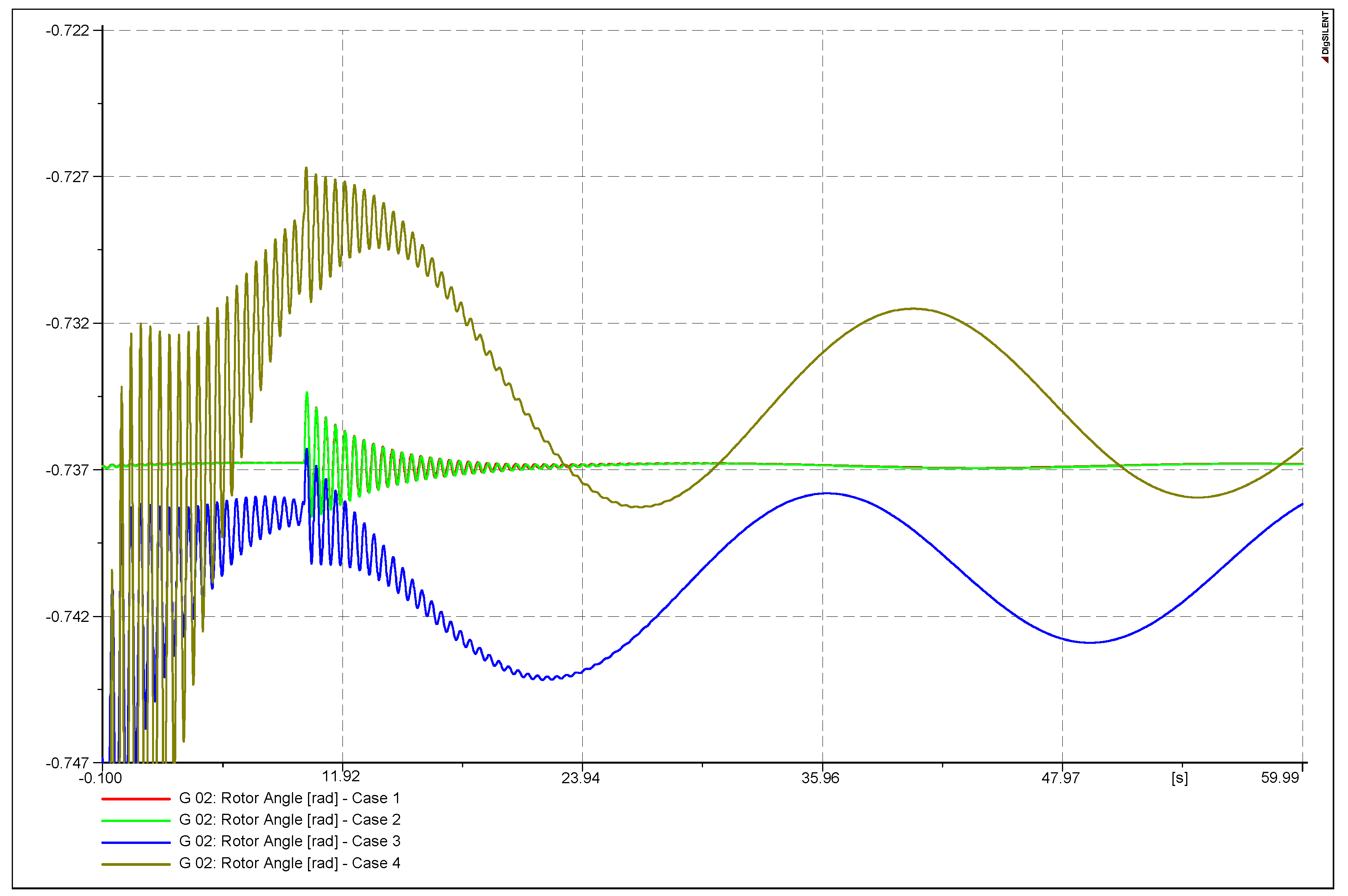
With respect to the damping percentages, when comparing all the modeled cases, there is a tendency in Cases 2, 3, and 4 to be less stable/steady. This is verified as the damping values are lower in the balanced case (Case 1). To check these results, the time domain simulation is carried out. A three-phase short circuit in bus 8 is activated at Second 10 of the simulation for one millisecond of duration. Figure 7 and Figure 8 show the resulting angle of the rotor and power delivery from Generator 2.

It is clearly visible that Cases 1 and 2 with the balanced initial condition are both stable. Cases 3 and 4 are stable, but the steady state performance has sustained variations.

The results obtained from Scenario 2 are presented in Figure 9, which shows the eigenvalues calculated with the Matlab software.

As was expected, the system tends to instability in all the cases due to the load increase (see

Table 6. Damping ratio percentages of Scenario 2.

Case 5		Case 6
Eigenvalues	Damping Ratio (%)	Eigenvalues	Damping Ratio (%)
−100.0005 ± 0.2310944i	99.9997	−100.0007 ± 0.2700379i	99.9996
−42.3731 ± 0.114598i	42.3728	−42.3731 ± 0.129702i	42.3727
−38.9105 ± 0.0353774i	38.9102	−38.9583	38.9579
−0.838697 ± 12.7151i	0.8387	−38.8626	38.8622
−0.20069 ± 8.3749i	0.2007	−1.6603 ± 15.7714i	1.6603
−4.9831	4.9830	−1.59423 ± 12.0215i	1.5942
−4.3417 ± 1.8695i	4.3417	−4.7451	4.7450
−4.2221 ± 1.7196i	4.2221	−4.4188 ± 1.9184i	4.4187
−4.2777 ± 1.8013i	4.2777	−4.2204 ± 1.7038i	4.2203
−3.3397	3.3397	−4.294 ± 1.8199i	4.2940
−1.3942	1.3941	−2.0724	2.0724
−1.2578	1.2578	−1.4928	1.4928
−0.7910	0.7910	−0.78907 ± 0.3786i	0.7891
−0.5069	0.5069	−1.2080	1.2080
−0.3246	0.3246	0.1771	−0.1771
−0.2232	0.2232	0.0002	−0.0002
−0.0045	0.0045	−0.3588	0.3588
−0.0282	0.0282	−0.2231	0.2231
−0.1003	0.1003	−0.1001	0.1001
−0.1001	0.1001	−0.1001	0.1001
−3.2258	3.2258	−3.2258	3.2258
Case 7		Case 8
Eigenvalues	Damping Ratio (%)	Eigenvalues	Damping Ratio (%)
−100.0007 ± 0.2706928i	99.9996	−100.0006 ± 0.248591i	99.9997
−42.3732 ± 0.132069i	42.3727	−42.3731 ± 0.106511i	42.3727
−38.9450	38.9446	−39.0035	39.0031
−38.8759	38.8755	−38.8172	38.8169
−1.66024 ± 15.7902i	1.6602	−1.76227 ± 15.8307i	1.7623
−1.54966 ± 12.1486i	1.5496	−2.05173 ± 11.6027i	2.0517
−4.7810	4.7809	−4.5189	4.5189
−4.4198 ± 1.9231i	4.4198	−4.4769 ± 1.9239i	4.4768
−4.2206 ± 1.7084i	4.2206	−4.2252 ± 1.686i	4.2251
−4.2954 ± 1.8199i	4.2954	−4.3212 ± 1.8441i	4.3212
−2.1211	2.1211	0.6634	−0.6634
−1.5075	1.5075	−1.8076	1.8076
−1.2391	1.2391	−1.4787	1.4787
−0.76142 ± 0.27743i	0.7614	−0.80976 ± 0.61076i	0.8098
0.1164	−0.1164	−0.8088	0.8088
0.0003	−0.0003	−0.3860	0.3860
−0.3678	0.3678	0.1447	−0.1447
−0.2336	0.2336	0.0001	−0.0001
−0.1001	0.1001	−0.1001 ± 1.5159 × ${10}^{-5}$i	0.1001
−0.1001	0.1001	−3.2258	3.2258
−3.2258	3.2258

). This indeed occurs with the classical model. However, with such representation, it is not possible to model an asymmetrical load distribution in the three phases. Scenario 2 is a load situation that stresses the operation of the system. Case 5 is stable, and the analysis of the eigenvalues shows that the system is on the verge of instability. The cases that used the proposed approach, Cases 6, 7, and 8, are unstable because all of them have real positive eigenvalues. This clearly means that the proposed model has opposite results to the classical analysis. The different load conditions of Cases 7 and 8 generate different results and show the unstable eigenvalue to be closer to the origin compared to Case 6.

Although Case 5 is stable despite the operation condition, it has very low damping percentages and is close to instability with the analytical model. The real time domain simulation of Scenario 2 showed that all of the systems were unstable in all conditions. This reinforces the idea that the classical model does not properly represents unbalanced conditions and that the proposed approach does a better performance.

To verify the instability in the time domain simulations, Figure 10 shows the frequency response for Cases 2 and 6. It is evident that Case 6 has an unstable condition as the frequency drops even without the short-circuit at Second 10. This behavior is identical in Cases 7 and 8.

5. Conclusions

The present research shows the necessary analytical methodology to carry out small signal stability studies in electric systems that operate in the unbalanced condition. In this context, a traditional testing system widely used in the international literature is used.

It is verified that the load variations and imbalances are increasingly more common in modern electric systems and cannot be represented by a classical model, which considers only one representation per phase because the analytical system does not show the imbalance present in the time domain simulations.

These results are particularly important in real systems where the imbalance can be present, such as distribution networks under different load conditions. For future work, it is intended to apply this model to real systems with a large number of variables and to consider the presence of self-sustained perturbations in time. The new approach presented in this paper to small signal stability analysis opens the way for the adjustment of the controller parameters in unbalanced multimachine systems.

Additionally, the research team is currently working on a generalized model, which allows including non-conventional renewable energies and aspects related to distributed generation so as to represent all the new elements influencing the stability of electrical power systems.

References

1. Kundur, P.; Paserba, J.; Ajjarapu, V.; Andersson, G.; Bose, A.; Canizares, C.; Hatziargyriou, N.; Hill, D.; Stankovic, A.; Taylor, C.; et al. Definition and classification of power system stability. IEEE Trans. Power Syst. 2004, 19, 1387–1401. [Google Scholar] [CrossRef]
2. Salim, R.; Ramos, R. A model-based approach for small signal stability assessment of unbalanced power systems. IEEE Trans. Power Syst. 2012, 27, 2006–2014. [Google Scholar] [CrossRef] [Green Version]
3. Miao, Z.; Choudhry, M.; Klein, R. Dynamic simulation and stability control of three-phase power distribution system with distributed generators. In Proceedings of the 2002 IEEE Power Engineering Society Winter Meeting. Conference Proceedings (Cat. No. 02CH37309), New York, NY, USA, 27–31 January 2002; Volume 2, pp. 1029–1035. [Google Scholar]
4. Xyngi, I.; Ishchenko, A.; Popov, M.; van der Sluis, L. Transient stability analysis of a distribution network with distributed generators. IEEE Trans. Power Syst. 2009, 24, 1102–1104. [Google Scholar] [CrossRef] [Green Version]
5. Spitsa, V.; Salcedo, R.; Ran, X.; Martinez, J.F.; Uosef, R.E.; De Leon, F.; Czarkowski, D.; Zabar, Z. Three–phase time–domain simulation of very large distribution networks. IEEE Trans. Power Deliv. 2012, 27, 677–687. [Google Scholar] [CrossRef]
6. Jain, H.; Parchure, A.; Broadwater, R.P.; Dilek, M.; Woyak, J. Three-phase dynamic simulation of power systems using combined transmission and distribution system models. IEEE Trans. Power Syst. 2016, 31, 4517–4524. [Google Scholar] [CrossRef] [Green Version]
7. Salim, R.H.; Ramos, R.A. A framework for analyzing the small signal dynamic performance of unbalanced power systems. IEEE Power Energy Soc. Gen. Meet. 2011, 1–8. [Google Scholar] [CrossRef]
8. Sun, J. Small-signal methods for AC distributed power systems-A review. IEEE Trans. Power Electron. 2009, 24, 2545–2554. [Google Scholar] [CrossRef]
9. Khazaei, J.; Miao, Z.; Piyasinghe, L.; Fan, L. Initialization of unbalanced radial distribution systems for small signal stability analysis. IEEE Power Energy Soc. Gen. Meet. 2015, 1–5. [Google Scholar] [CrossRef]
10. Nasr-Azadani, E.; Canizares, C.A.; Olivares, D.E.; Bhattacharya, K. Stability analysis of unbalanced distribution systems with synchronous machine and DFIG based distributed generators. IEEE Trans. Smart Grid 2014, 5, 2326–2338. [Google Scholar] [CrossRef]
11. Azadani, E.N.; Canizares, C.; Bhattacharya, K. Modeling and stability analysis of distributed generation. In Proceedings of the 2012 IEEE Power and Energy Society General Meeting, San Diego, CA, USA, 22–26 July 2012; pp. 1–8. [Google Scholar]
12. Wen, B.; Boroyevich, D.; Burgos, R.; Mattavelli, P.; Shen, Z. Small-Signal Stability Analysis of Three-Phase AC Systems in the Presence of Constant Power Loads Based on Measured d-q Frame Impedances. IEEE Trans. Power Electron. 2015, 30, 5952–5963. [Google Scholar] [CrossRef]
13. Mortazavian, S.; Shabestary, M.M.; Mohamed, Y.A.R.I. Analysis and Dynamic Performance Improvement of Grid-Connected Voltage-Source Converters under Unbalanced Network Conditions. IEEE Trans. Power Electron. 2017, 32, 8134–8149. [Google Scholar] [CrossRef]
14. Karami, E.; Gharehpetian, G.B.; Madrigal, M.; De Jesus Chavez, J. Dynamic phasor-based analysis of unbalanced three-phase systems in presence of harmonic distortion. IEEE Trans. Power Syst. 2018, 33, 6642–6654. [Google Scholar] [CrossRef]
15. Miao, Z.; Piyasinghe, L.; Khazaei, J.; Fan, L. Dynamic Phasor-Based Modeling of Unbalanced Radial Distribution Systems. IEEE Trans. Power Syst. 2015, 3, 3102–3109. [Google Scholar] [CrossRef]
16. Ojo, Y.; Schiffer, J. Towards a time-domain modeling framework for small signal analysis of unbalanced microgrids. In Proceedings of the 2017 IEEE Manchester PowerTech, Manchester, UK, 18–22 June 2017; pp. 1–6. [Google Scholar] [CrossRef] [Green Version]
17. GmbH, D. DigSilent PowerFactory 2019 User Manual; McGraw-Hill: New York, NY, USA, 2018. [Google Scholar]
18. Sauer, P.W.; Chow, J.H. Power System Dynamics And Stability, 2nd ed.; Wiley: Hoboken, NJ, USA, 2007. [Google Scholar]
Figure 1. Model of the two axes used in the modeling.
Applsci 10 08855 g001
Figure 2. Circuit of the negative sequence for the multimachine generator case.
Applsci 10 08855 g002
Figure 3. Circuit of the zero sequence for the multimachine case generator.
Applsci 10 08855 g003
Figure 4. Nine-bus testing system.
Applsci 10 08855 g004
Figure 5. Diagram of the methodology flow used in the case simulation.
Applsci 10 08855 g005
Figure 6. Eigenvalues obtained from the normal case modeling.
Applsci 10 08855 g006
Figure 7. Angles of Machine 2 in the first scenario.
Applsci 10 08855 g007
Figure 8. Active power for Machine 2 in the first scenario.
Applsci 10 08855 g008
Figure 9. Eigenvalues resulting from the modeling of the case with a 45% increased load.
Applsci 10 08855 g009
Figure 10. Angles and frequency of Machine 2 in Case 2 versus Case 6.
Applsci 10 08855 g010