Abstract
Soft-landing on planetary surfaces is the main challenge in most space exploration missions. In this work, the dynamic modeling and simulation of a three-legged robotic lander based on variable radius drums are presented. In particular, the proposed robotic system consists of a non-reversible mechanism that allows a landing object to constant decelerate in the phase of impact with ground. The mechanism is based on variable radius drums, which are used to shape the elastic response of a spring to produce a specific behavior. A dynamic model of the proposed robotic lander is first presented. Then, its behavior is evaluated through numerical multibody simulations. Results show the feasibility of the proposed design and applicability of the mechanism in landing operations.
1. Introduction
In space exploration, landing on a planet, an asteroid or any other celestial body is an extremely important task and can determine the success or the failure of the entire mission. In the past decades, many missions failed due to the crash of the lander to the ground during this delicate operation. Despite these failed missions, many other missions succeeded and over the years many systems were tested and employed to achieve a soft landing.
The most remarkable mission, known as Apollo 11, from the NASA Agency, had the objective to land a probe transporting humans for the first time on the Moon’s surface. Successful landing was obtained first by executing a powered descent maneuver. Then, successful touchdown was achieved by means of a suspension system having a honeycomb shock absorber on each lander-leg strut [1]. During the Vikings mission started in 1975, two twin probes named Viking 1 and Viking 2 were sent to Mars. The landers of the two probes were legged, and a combination of parachute and rocket propulsion was used to achieve soft-landing on the planet surface [2]. The same operations were implemented for the lander used in 1997 for the Cassini–Huygens NASA-ESA-ASI mission, which landed successfully on Titan, one of the moons of Saturn. After the Viking mission, NASA sent further probes to investigate Mars planet. First, it was the turn for NASA’s Pathfinder mission, which started in 1996 [3]. Then, in 2004, the NASA’s Mars Exploration Rovers Spirit and Opportunity were sent to the red planet. In these three missions, a system based on gas-filled airbags was adopted to achieve soft-landing [4]. Another remarkable mission was the Mars Science Laboratory, which deployed successfully the lander Curiosity on the Mars surface in 2011. Successful landing was achieved by adopting a combination of parachute, rockets, and the Sky Crane system. More recently, the Rosetta mission from ESA used a powered descend to land on the comet and a system of anchors to remain attached to it once controlled impact occurred [5].
In parallel to NASA, during the Space Race, the Soviet Space Program, starting with impactors [6], implemented several innovations which led to the first-ever soft-landing on another planet with the lander Luna 9 in February 1966 [7]. In 1970, the Soviet Lunokhod 1 was the first successful rover to land on another planetary body [8]. In the 1990s, the Chinese space agency (China National Space Administration) started a program which enabled the soft-landing of the Chang’e 3 lunar lander and rover Yutu in December 2013 [9]. The lander Chang’e 4 followed in January 2019 [10].
In past years, many authors have studied the problem of soft-landing of landers in different fields. For example, Wang et al. in 2019 studied the use of magnetorheological fluid dampers with semi-active control on damping force in order to adjust to landing conditions [11]. Furthermore, the shock absorber design [12] and the lander stability [13] have been investigated numerically by mean of optimization algorithms. Moreover, legged landers with capabilities of walking on planet surface after the landing have been studied in [14,15].
Two main problems can be addressed to the study of soft landing operations: the modeling of the system dynamics, and the modeling of the interactions between the lander and the soil. Several authors tried to study the soft landing problem by means of simulation software, and chose as a case study a four-legged lander. For example, Xu et al. in 2011 simulated the soft-landing of a lunar lander first using MSC-ADAMS considering the lunar soil as a rigid body, and then MSC-DYTRAN considering the lunar soil as a flexible body [16]. Wan et al. in 2010, chose MSC-DYTRAN to simulate soft-landing of a lunar lander with the finite elements method and a nonlinear transient dynamics approach [17]. Zheng et al. in 2018, simulated the impact of a legged lander using explicit finite element analysis using LS-DYNA and ABAQUS softwares [18]. Liang et al. in 2011, used an explicit nonlinear finite element method implemented in ABAQUS to study the impact of a legged lander and aluminum honeycomb shock absorber with the lunar soil [19]. Other authors in [20,21,22,23,24] studied the impact of the lander with ADAMS considering the soil either as an elastic or a rigid body.
In this paper, we present the dynamic modeling and simulation of a robotic lander, based on variable radius drums (VRDs), which inherits from the concept outlined by Seriani in [25]. The proposed mechanism consists of a non-reversible mechanism that allows a landing object to decelerate in the phase of impact with ground. A VRD is a device characterized by the variation of the spool radius along its profile, as defined by Seriani and Gallina in [26]. In this context, it is used to ensure a constant force and a controlled deceleration of the structure during landing. VRDs were studied for many applications, as, for instance, in gravity-compensation systems [27], to guide a load along an horizontal path, or to improve locomotion of a legged robot [26]. Scalera et al. in 2018, studied a cable-based robotic crane based on VRDs capable of moving a load through a planar working area [28]. Moreover, Fedorov and Birglen in 2018 employed two antagonistic VRDs in a cable-suspended robot to steer the end-effector along a desired pick-and-place trajectory. The same concept was also adopted for the static balancing of a pendulum [29]. In these cases, the rationale for the use of the VRD is to generate geometrical trajectories in a mechanism. Conversely, in this work we employ a synthesized VRD to generate a specific force when connected to a linear spring-loaded mechanism. Other examples of the application of VRDs, also known as non-circular pulleys, include cable actuation in soft robot joints [30], devices for upper leg rehabilitation [31], mechanisms for energy saving [32], and force regulation [33].
When landing on celestial bodies, the ground characteristics are an important influence on the mission [34], and as such many attempts are made to determine them in advance [35,36]. Many works detail the soil characterization, in particular concerning its granulometry [37]. In order to build the simulations on a solid baseline, we used an experimental approach to the determination of the characteristics of the soil; a basaltic sand of volcanic origin with average grain size range of 3 to 5 mm which pertains to the coarse sands as described by NASA [38,39].
The main contributions of this paper can be summarized as follows; the design and the numerical validation of a three-legged robotic lander for space applications. The landing mechanism leverages a passive mechanism for impact energy absorption, which is based on VRDs and cables to transfer the impact energy to a preloaded spring. Moreover, the presented passive mechanism is able to ensure a controlled force and acceleration of the structure, thus preventing damage to the supported payload due to high accelerations. We believe this kind of system can find application in real and concrete scenarios considering its reusability, its high payload/lander mass ratio, and its modularity.
Compared to relevant literature, and in particular the work of Seriani [25] which implements an ideal linear spring–damper contact and ideal Coulomb friction models, this work presents several novelties: it provides an experimental determination of the characteristics of soft basaltic sand soil for implementation in a spring–damper ground contact as well as implementing a nonlinear stiffness model; furthermore, it implements experimentally defined static and dynamic friction coefficients. In addition, the numerical implementation of the theoretical model is more stable and thus avoids the implementation of numerical damping of the legs rotation. Moreover, in this work in the 3D lander three ratchets are introduced, functioning as retention mechanisms that make the system non-reversible. In particular, their role is to limit the return rotation of the legs once they are fully rotated and the payload is completely decelerated; this keeps the lander from bouncing after landing. Additionally, limiting the rotation altogether, it forces the lander to keep its center of mass closer to the ground, thus increasing stability. Moreover the ratchets prevent the discharge of the energy stored in the preloaded springs, thus avoiding high bounces of the lander.
The rest of the paper is organized as follows. In Section 2, the dynamic modeling of the robotic lander based on VRDs is introduced, whereas in Section 3, the setup of the ADAMS numerical simulations is explained. Section 4 reports the simulation results for two test cases: the impact on an horizontal surface and the impact on an inclined surface. In Section 5, the results are discussed and compared with the theoretical model. Finally, the conclusions are given in Section 6.
2. Dynamic Modeling of the Robotic Lander
The lander structure studied in this work is based on the concept outlined in [25]. In addition, a ratchet mechanism is introduced to block the rotation of the legs when the structure of the lander starts to move upwards at the end of the deceleration phase. As shown in Figure 1, the lander is composed of three legs arranged with an angle of 2/3 π from the others and having a fixed offset from the center of mass of the lander, and of an hexagonal body on which the payload is fixed. From Figure 1, it can be seen that the lander is symmetrical with respect to a vertical axis passing through its center of mass. Therefore, to define the dynamics of the system, a simplified model of a third of the lander is considered.
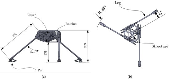
Figure 1.
The computer-aided design (CAD) model of the proposed three-legged lander, along with labels for its main parts and main dimensions: (a) lateral view and (b) top view.
2.1. Variable Radius Drum Mechanism
A schematic view of the lander-leg mechanism at the beginning of the impact is illustrated in Figure 2. The main parts composing each lander-leg mechanism are a leg, a fixed radius pulley with radius , attached to the leg, a VRD, another fixed radius pulley with radius , attached to the VRD, and a preloaded spring. Moreover, two cables are used in the mechanism. The extremities of the first cable are attached to the VRD and to the fixed radius pulley (red line in Figure 2). The extremities of the other cable are attached to the preloaded spring, which is connected to the lander chassis, and to the fixed radius pulley connected to the VRD (green line in Figure 2). This specific layout allows the VRD to shape the elastic response of the preloaded spring. More precisely, the preloaded spring generates a reactive torque M acting on the fixed-radius pulley attached to the leg. As the response of a preloaded spring is discontinuous, the reactive torque M can be approximated by the following continuous and differentiable function [25,40,41],
where is the preloaded torque, f an approximation factor, k the spring stiffness, and the relative rotation of the leg from its rest position .
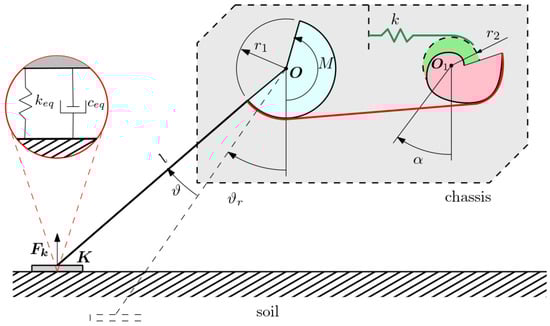
Figure 2.
Schematic view of the lander-leg mechanism at the beginning of the impact with soil with detailed view of the model of the normal contact force as a spring–damper system.
In the following, the profile of the VRD is synthesized as explained in [26,28] in order to guarantee a constant force acting on the pads of the lander during the deceleration phase, that is, A generic point of the VRD profile , expressed in its local coordinates, is defined by
where , with reference to Figure 2, is the relative rotation of the VRD; is the distance between the point and the idle pulley center O, expressed by
where is a generic rotation matrix, and is defined as
With reference to Figure 2, is defined as the distance between O and , whereas is the cable wound function. In order to synthesize the VRD for this application, the expression of the cable wound function and its first- and second-order derivatives with respect to need to be derived. From Figure 2, the wound cable function and its derivatives assume the following expressions.
By looking at Figure 2, and by applying the principle of virtual works, it is easy to demonstrate that the derivative of with respect to is
where is the force exerted by the preloaded spring. Starting from Equation (6) and its second-order derivative, it is possible to synthesize the VRD, given the pad–soil contact force .
2.2. Dynamic Model
The dynamic model of the system can be obtained by considering only a third of the lander thanks to its axial symmetry. A bidimensional model is considered and the displacement of the lander is constrained to be only along the vertical axis. As a starting point for the definition of the dynamic model, the kinetic energy of the system is computed as follows,
where m is the mass of the lander, x is the vertical displacement of its center of mass, is the moment of inertia of the leg computed in its center of mass, is the mass of the leg, and l is the leg length. The potential energy of the system accounts for the gravitational terms of the leg and the structure and the nonlinear response of the VRD, modeled as a nonlinear torsional spring. It results as
where is the gravitational force field. The considered model is a single-degree-of-freedom model. The generalized coordinate is chosen to describe the entire mechanical system. Then, by defining the Lagrangian function as , the Lagrangian equation can be written. This results in a second-order ordinary differential equation that represents the equation of motion of the system, as follows,
where and are the Lagrangian components of the i-th conservative and j-th non-conservative forces, respectively, which are not directly included in the Lagrangian function. In this specific case, those forces contains the components of the contact forces that take place between the lander pad and the ground. The contact force is composed by the normal and frictional components whose modeling is explained in detail below. Note that the generalized force for a given force , with point of application , and a generalized coordinate q is expressed as follows,
Equation (9) is obtained using Equations (7), (8), and (10), and represents the dynamic model of the lander in the phase of impact with ground. The dynamic model of the lander for the phase between the release of the lander and the touchdown is the one for a free falling object. This model is used to compute the state variables of the lander at the end of the free falling stage, i.e., the beginning of the impact problem. These computed states becomes the boundary initial conditions for the ordinary differential equations resulting from Equation (9). The main effect of the VRD is to generate a nonlinear torque applied to the leg joint in order to keep constant the force acting on the pads of the lander. The nonlinear torque obtained from the VRD synthesis is shown in Figure 3.
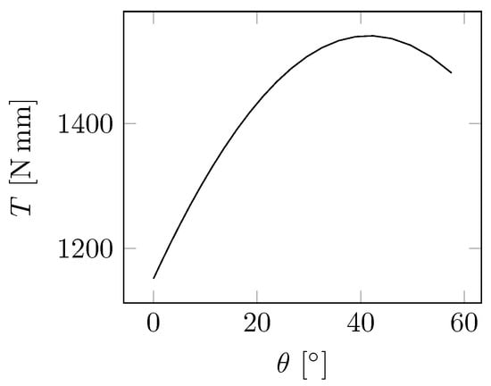
Figure 3.
Nonlinear, softening, spring response obtained from VRD synthesis.
2.3. Soil Characterization
In order to completely define the dynamic model of the lander, the properties of the soil need to be analyzed.
In this work, we consider a single type of soil whose characteristics are determined experimentally; while mission-specific conditions of the ground can differ greatly, in this preliminary phase of experimentation we have elected to consider only one type.
In particular, the normal contact force between the pads of the lander and the soil is modeled as a non-linear spring damper system as depicted in Figure 2, and is described by the following [13],
where is the equivalent stiffness of the soil, is the equivalent damping factor of the soil, the force exponent responsible of the nonlinear behavior of the spring, and x and are the depth and the speed of penetration of the pad into the soil, respectively. In contacts problems a further force that plays an important role is the frictional force acting between the pad and the soil. In this context, the Coulomb friction model is used, whose expression is reported in
where is the speed acting along a plane parallel to both the surfaces in contact, N is the normal force acting between the parts in contact and having direction coincident with the normal of the previously defined plane, is the static friction coefficient, and is the dynamic friction coefficient.
In order to conduct accurate and comparable simulations, the parameters , , , and need to be estimated. For what concern the parameters that describe the nonlinear spring damper system, some preliminary tests have been performed to estimate the modulus of subgrade reaction k. This can be considered directly related to the soil equivalent stiffness and is defined as follows,
where q is the applied pressure and is the penetration depth. More precisely, the test is conducted as follows; a circular plate with dimensions comparable with the lander pad, is positioned on the flat sample soil surface. Subsequently, a 1 kg steel weight is positioned above the circular plate and the deflection at static conditions is measured. The measures, as the deflections are truly little and submillimeter, are taken by mean of image analysis. Comparison between the pictures taken before applying the load and the one taken after the load is applied is done, as can be seen in Figure 4b. The aforementioned test is repeated 13 times, and the measured penetration depth is found to be . Therefore, choosing the penetration depth to be the mean value and by using Equation (13), it is possible to estimate the modulus of subgrade reaction k and then by geometric considerations estimate the soil equivalent stiffness [22]. The equivalent stiffness is then estimated to be . Finally, the equivalent damping factor instead is estimated as of the equivalent stiffness factor [22]. Thus, in this work we have assumed .
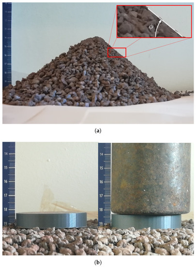
Figure 4.
Experimental characterization of the soil: (a) measure of the internal angle ; (b) measure of the penetration depth. The scale unit is centimeters in both images.
For what concerns the second kind of parameters which describe the friction model, in a first analysis the static friction coefficient can be estimated as , where is the internal friction angle of the soil. The angle has been measured experimentally by conducting 15 tests. More precisely, the test is conducted as follows; a small quantity of the sample soil is slowly poured on a flat surface, and a picture of the heap vertical profile is taken. At this point, the internal angle of the soil is determined as can be seen in Figure 4a and is found to be . We elected the angle to be the mean value, consequently .
Kinetic friction coefficient on the other hand is assumed to be a fraction of the measured static friction coefficient. In this case, .
All the required lander design parameters are summarized in Table 1. Considering that every part of the lander is fabricated in Polylactic Acid (PLA) polymer, the inertial parameters can be computed, and it is possible to solve the ordinary differential equation resulting from Equation (9), and then evaluate the contact force, which is required for the synthesis of the VRD.

Table 1.
Parameters used in the design of the lander.
3. Simulated Test Bed
In this section, the modeling of the multi-body system (MBS) representing the lander and the setup for the numerical simulations are presented. Both the entire lander model and the soil are modeled, respectively, as a MBS and a rigid body, and the result of this modeling process can be seen in Figure 5.
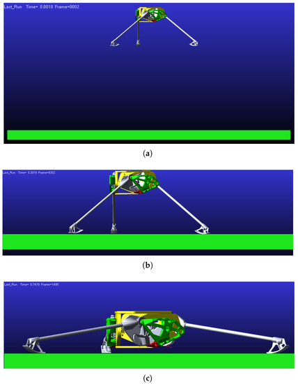
Figure 5.
View of the lander MBS and the soil modeled in ADAMS: (a) the initial condition of the simulation; (b,c) the lander configuration at the beginning and at the end of an impact simulation on a flat surface, respectively.
The MBS representing the lander model is constructed by connecting, with appropriate joints, each single rigid body which is functional to the correct behavior of the global system. The functional bodies, which globally compose the MBS of the lander, are the lander hexagon structure, its three legs, the three ratchet mechanisms and finally the three covers, respectively, indicated in yellow, gray, red, and green in Figure 5 and Figure 6. Their geometrical properties are summarized in Table 2, whereas the joints between the parts are summarized in Table 3. It is important to report that the non-functional parts of the lander together with the payload are included in the model by adding their mass properties to the lander structure body. Moreover, the joints used are considered as ideal joints, i.e., without considering friction and deformations.
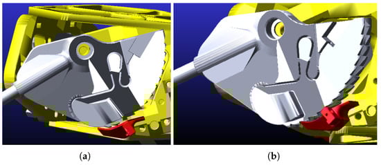
Figure 6.
View of the leg joint and the ratchet mechanism used in ADAMS. (a) The ratchet and the leg joint at rest position; (b) the ratchet blocking the opposite rotations of the leg thanks to the contact force between the ratchet and the leg.
Table 2.
Geometrical properties of the main functional rigid bodies composing the lander MBS model. All the inertia components are expressed in kg mm2.
Table 3.
Joint type used between each pair of rigid bodies.
Finally, for what concerns the soil rigid body, it is modeled as a box having dimensions and positioned below the lander structure center mass.
Once all the bodies and their joints are defined, forces acting on the model should be added. These forces can be split up between external forces and contact forces. The external forces implemented in the simulation environment are a gravitational force field, a linear torsional spring between each ratchet and the structure, and a nonlinear torque applied between each leg and the lander structure. The linear torsional spring between each ratchet and the structure is introduced in order to simulate the elastic deflection of the ratchet from its rest position. In order to provide values that describe the torsional spring, the ratchet is considered as a cantilever, which deflects under the action of the contact force between the ratchet and the leg. Therefore, by using the elastic theory, it is possible to define an equivalent torsional stiffness coefficient for the spring, whose expression is . E is the Young elastic modulus of the PLA, I is the moment of inertia of the resistant cross-area of the ratchet, and l is the length of the cantilever. Finally, a stiffness coefficient of k = 288 N mm rad−1 is set for the springs. The nonlinear torsional spring between each leg and the structure is introduced in order to simulate the resistant torque applied to the leg joint generated by the action of the VRD pulley, as stated in Section 2. For the implementation in ADAMS, instead of using directly Equation (1), a cubic interpolating polynomial function is used in order to approximate the response of the VRD pulley, with coefficients , , , and .
The contact forces implemented in the simulation environment are the forces between each leg and the ratchet next to it, the forces between each leg and the cover next to it, and those between each leg and the soil. Every contact is defined as a solid-to-solid contact force which is composed by a normal contact force following the relation shown in Equation (11), and a frictional force following the Coulomb model Equation (12).
The definition of contacts between the legs and the ratchets is fundamental for the correct functioning of the retention mechanism. In particular, when the structure is decelerating, the leg rotates in the admissible direction and this force makes the ratchet to bend, allowing the leg to rotate. When the structure stops its deceleration and starts to move upwards, instead, the tip of the ratchet mechanism connects with the tooth present on the side of the leg joint, allowing the ratchet to limit the opposite rotation of the leg joint. This can be immediately seen from Figure 6a,b. The contacts defined between the legs are required to implement a physical lower end-stop to the revolute joint connecting the leg to the structure. By looking at Figure 6a,b, on the side surface of the leg joint a small part is modeled which goes in contact with the cover and thus limits the joint rotation. Finally, the contacts between the box model representing the soil and each of the three legs are the most important actors for the whole soft-landing simulation and need to be modeled accurately. The parameters that need to be set for the contact are the stiffness coefficient, the nonlinear force exponent, the damping coefficient, the penetration depth, and the static and dynamic friction coefficients. The parameters have been estimated in Section 2.3.
4. Simulation Results
In this section, we present the numerical simulations that are conducted on the model of the three-legged lander prototype. The dynamic behavior of the system is simulated using the multi-body software MSC ADAMS 2019. Two simulated cases are considered in this work:
- Case (1): impact simulation on flat surface. In this simulation the behavior is investigated of the lander free-falling from a fixed height and impacting on a flat horizontal surface. In particular, we analyze the contact force distribution, the lander deceleration, the angular displacement of the leg, and the ratchet action.
- Case (2): topple simulation. In this simulation, the behavior is investigated of the lander impacting on an inclined surface, after a free-fall from a fixed height. Subsequently, the critical angle is found at which the lander topples.
4.1. Case (1): Impact Simulation on Flat Surface
In this simulation, the lander is let free to fall from a fixed height and impacts with the box representing the soil model. Figure 5a–c shows the initial, impact moment, and final configurations, respectively, of the lander MBS in the simulation over a flat surface. In this case, a trial and error strategy is adopted, in order to investigate the maximum admissible drop height and considering the payload of the lander to be 0.5 kg. Moreover, in this subsection the most representative results that are obtained for the maximum drop height, which is found to be H = 0.45 m, are reported. A simulation duration of 1 s has been determined, as it is enough to catch the transient phenomenon taking place between the beginning of the simulation and the lander MBS stabilization.
Figure 7a–c reports, respectively, the lander MBS center of mass displacement, speed, and acceleration along the vertical axis, that is the axis of motion of the free falling lander. Figure 8a–c reports, respectively, the rotations of each of the leg structure joints, the torque generated by each of the three VRDs, and the contact forces exerting between each pad and the soil during the soft-landing simulation. Finally, Figure 9a,b shows the rotations of each of the ratchet structure joint and the evolution of the kinetic energy of the lander MBS.
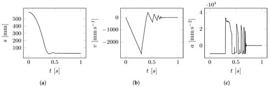
Figure 7.
Information about the state of the lander’s MBS along the vertical axis: (a) the displacement of the center of mass; (b) the velocity; (c) the acceleration.
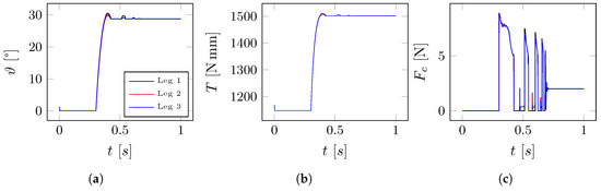
Figure 8.
(a) The curves representing the angular rotation of each of the three leg structure revolute joint; (b) the curves representing the torque response of each of the three VRD’s; (c) the curves representing the contact force between each of the legs with the soil.
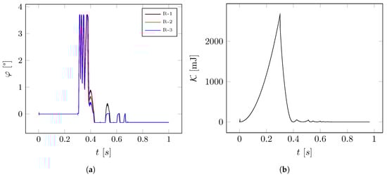
Figure 9.
(a) The rotation evolution of each of the ratchet-structure joint; (b) the kinetic energy evolution over time of the lander MBS.
4.2. Case (2): Topple Simulation
In this section, the case of topple simulation is investigated. More precisely, the aim of the numerical tests is to identify at which ground surface angle the lander topple. This angle is named landing critical angle . To achieve this, the same model used from the previous analysis is considered. For every simulation, the model of the ground is rotated by increasing angles around the z axis, and rigidly translated along the y axis in order to keep the drop height constant. The simulations of Case (2) allow to investigate the range of admissible slope angles to achieve safe soft-landing without the lander toppling. It is important to say that all the simulations are conducted using the same maximum drop height of H = 0.45 m. By pursuing this strategy, it is found that the lander topples at a critical landing angle , as it can be seen in Figure 10. Moreover, some important results for the sample case of an inclined plane simulation with an inclination ratio 1:5 are reported.
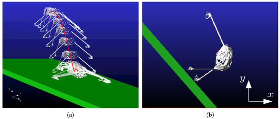
Figure 10.
(a) A time-series representation of the simulation for the lander MBS soft-landing conducted on an inclined surface; (b) the lander MBS toppling at the landing critical angle .
Figure 11a–c reports the lander MBS center of mass displacement, speed, and acceleration along the three axes, respectively. Figure 12a–c reports the rotations of each of the leg structure joints, the torque generated by each of the three VRDs, and the contact forces exerting between each pad and the soil during the soft-landing simulation, respectively. Finally, in Figure 13 the evolution of the kinetic energy of the lander is shown.
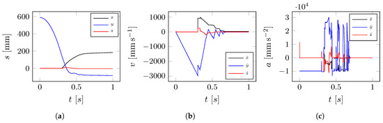
Figure 11.
Information about the state of the lander’s MBS along the vertical axis: (a) the displacement of the center of mass; (b) the velocity; (c) the acceleration.
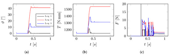
Figure 12.
(a) The curves representing the angular rotation of each of the three leg structure revolute joint; (b) the curves representing the torque response of each of the three VRD’s; (c) the curves representing the contact force between each of the legs with the soil.
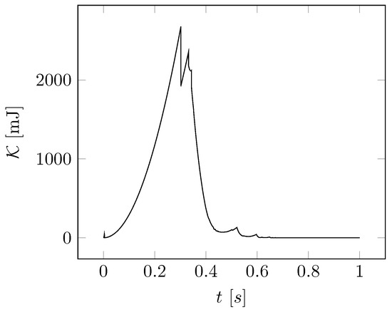
Figure 13.
Kinetic energy evolution over time of the lander MBS.
5. Discussion
In this section, the results obtained from the simulations of soft-landing on a flat surface and an inclined surface, reported in Section 4.1 and Section 4.2, are discussed. Moreover, some important results obtained with the MATLAB-based numerical integration of the theoretical model developed in Section 2 are reported in order to validate the approach.
5.1. Comparison with the Theoretical Model
Comparisons of the ADAMS simulations with the theoretical model are conducted for two different cases regarding the analytical-based simulation. For the first case, a length of the lander leg equal to is chosen, which corresponds to the conservative value chosen, i.e., the distance from the lander joint axis from the pad closest contact point. For the second case, a length equal to is chosen, which corresponds to the mean distance of the contact point from the joint axis. This is because despite the analytical model, in which the pad is considered a point, the pad in the ADAMS model is a rigid body having its own semicircular geometry. Therefore, while in the analytical model the contact point is always at a fixed distance from the lander joint axis, the geometry of the pad leads to the fact that the contact point keep varying all along the pad profile during the whole contact phase, thus changing the arm lever.
The comparisons are conducted in the scope of the Case (1). Moreover, in order to catch the influence of the ratchets in the global dynamics of the lander, an additional simulation in ADAMS without ratchets is conducted and compared with the others. Figure 14 shows the comparison between the ADAMS simulations and the MATLAB-based analytical simulation for the two leg length value chosen: in the top row the acceleration of the lander is compared, in the middle row the contact force acting between the soil and the lander pad is compared, and in the bottom row the leg-joint rotation is compared. The black curves represent the ADAMS simulations with the ratchet (ADAMS-R), the blue curves represent the ADAMS simulations without ratchets (ADAMS-NR), and finally the red curves represent the simulations based on the analytical model described in Section 2. It is important to remark that the figures refer only to the first bounce of the lander. This is because the lander behavior is different between the simulations after the first bounce. In fact, the analytical model does not implement the ratchet. In ADAMS, on the other hand, this mechanism is present and it affects the behavior of the system after the deceleration phase.
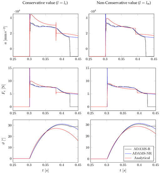
Figure 14.
Comparison between ADAMS simulations with and without ratchets and the MATLAB-based analytical simulation for two leg length parameter chosen: in the top row the lander acceleration, in the middle row the contact force between soil and lander pad, and in the bottom layer the evolution of the leg joint rotation.
By comparing the curves, similarities in the trends and with the values assumed can be found. More precisely, with the theoretical model the deceleration of the lander during impact assumes values for a leg length equal to and values for a leg length equal to , whereas with the simulation in ADAMS an acceleration is observed. The same can be observed with the contact force and the leg joint rotation; in particular a contact force has been observed using the theoretical model and the same is observed in the in ADAMS simulation. Finally, for what concerns the leg joints rotation, it can be seen that in both the theoretical model simulation as well as in the ADAMS simulations, the maximum rotation of the joints reaches a value slightly below . The discontinuities visible in the ADAMS simulation black curves visible from the acceleration and force graphs are due to the action of the ratchets which limits the rotation of the lander legs; in fact, in the curves representing the analytical model (which does not implement the action of the ratchet), these same discontinuities are not present.
By comparing the MATLAB-based simulations of the left column with the right column of Figure 14, it can be noticed that the leg length parameter used for the theoretical model, i.e., the distance of the contact point of the pad from the joint axis, has a great influence on the curve’s trend of the analytical model. In fact, by using as leg length , the analytical curves better fits the ADAMS ones, especially for the contact force. However, at the beginning of the impact, the analytical curve has a greater peak with respect to the ADAMS ones; this is because at that stage the contact point is further from , and as the impact time goes on, and the legs rotates the contact point comes closer to the mean point until the minimum distance is reached.
By comparing the black curves with the blue curves in Figure 14 it can be clearly seen the influence of the ratchet to the global dynamics of the lander. In particular, from the force and acceleration graphs small humps in the curves can be recognized due to the presence of the ratchet. From the angle graphs, instead, it can be clearly seen the influence of the ratchet: in particular as it exerts a reactive torque which opposes to the leg opening during landing, this leads to the leg opening with a lower angle. It is important to remark that the ratchet has been modeled in order to easily deflect, so in this case the influence of the ratchet is present but it does influence to a lesser extent the global dynamics of the lander. The stiffer the ratchet is, the more it influences the dynamics of the lander, even leading to the limit case of no opening of the legs at all thus imposing enormous vertical accelerations to the structure and the payload.
An other cause which we can address the discrepancies between the MATLAB-based analytical simulation and ADAMS ones is one which is due to the limit that the analytical model is a purely bidimensional model, thus unable to catch 3D related phenomenon. Of particular note is that during the soft-landing the lander structure body slightly rotates around it’s vertical axis (allowed given the lander legs configuration), thus part of the lander energy is split into rotational energy and therefore dissipated through lateral friction forces. This just being said can be seen from Figure 15 which shows in the left the lander rotation and in the right its rotational speed during the impact stage. During this stage can be recognized that in 0.15 s the lander rotational energy is almost completely dissipated. Moreover, an other factor which causes discrepancies between the models is that ADAMS implements a nonlinear damper in the contact model; while the analytical model implements a linear damper. This fact causes differences at the initial stage of the contact. In fact the purely linear damper causes greater damping forces in the moment of contact. Namely, the combination of all the factors mentioned above leads to discrepancies between the analytical model and the ADAMS simulations. However, despite the discrepancies between the ADAMS simulations and the analytical model, which after all is a bidimensional idealization of a three dimensional lander, the results of the two models show remarkable adherence, thus validating the approach.
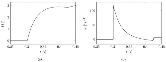
Figure 15.
(a) The lander structure center mass rotation around its vertical axis and (b) its angular speed around the same axis.
5.2. Case (1): Simulation on Horizontal Surface
Figure 7 reports the evolution of the state of the lander MBS during the simulation time. In Figure 7a the loss of height can be seen; Figure 7b shows the evolution and the changes of speed the lander is subjected; finally Figure 7c describes the acceleration of the lander. From these figures it can be seen that at s, the lander impact the ground with a speed ms−1. Moreover, some sudden changes in speed are observed, which identifies the bounces of the lander after impact. The oscillation speed and amplitude decreases due to the dissipative forces defined in the contact problem. It can be seen that the lander is subjected to peaks of deceleration having amplitude . It is important to report that the evolution of the acceleration has been slightly filtered in order to cut out the high-frequency peaks of deceleration taking place in specific instants of time due to numerical instabilities. Disregarding these is allowed from a simulation perspective, as their impact on the landing behavior is low and they can easily be filtered out with dampers on the payload attachment points.
When the lander impacts with the soil its legs start to rotate due to the torque generated by the contact force with the ground. As expected, for an impact simulation on an horizontal surface, the legs of the lander rotate uniformly, until the maximum angle for each leg. The reactive torques generated have the same trend. These aspects can be observed in Figure 8a,b. From the same figures, the action of the ratchets can be observed. More precisely, when the leg rotation reaches its maximum value, the leg starts to rotate back to the original position. However, the ratchet almost immediately engages and limits this motion, effectively stopping the leg orientation at the current angle; to this angle a fixed torque of Nm is naturally associated. Finally, in Figure 8c the contact forces acting between the soil and the lander leg are shown. In a way similar to the case of acceleration, the contact forces have been slightly filtered in order to remove the high-frequency spikes. In this figure the bounces can be seen and, as expected, the contact force has the same trend as the joint rotation. By looking again at the figure we can say that the first peak of the contact force is the one responsible of dissipating most of the energy of the system, as can be seen in Figure 9b, which represents the kinetic energy of the lander MBS during the whole impact simulation. The other spikes are about the lander stabilizing on the soil surface. However, the amplitude of the contact force is . Finally, Figure 9a reports the rotation of the ratchet structure revolute joint. The high peaks represent the instants at which the ratchet overcomes the tooth present on the side of the leg, and thus moving to the next tooth. In this case, the ratchet overcomes four teeth. The low peaks instead are due to the leg trying to rotate in the opposite direction, against the engaged ratchet.
5.3. Case (2): Topple Simulation
In the following, the results of an inclined surface sample impact simulation with an inclination of 1:5 are discussed. We disregard the ratchet structure joint rotation. Differently from Case (1), in which the state of the lander was changing only along the vertical axis, in this simulation the state of the lander changes along the other two directions as well. In Figure 11a, the displacement is reported of the lander center of mass along the three directions. In Figure 11b, we can see the speed of the lander along the three directions. Figure 11c shows the acceleration of the center of mass of the lander along the three directions; this has been slightly filtered in order to remove the high-frequency high spikes. While the main component of motion remains along the vertical axis, in this case the others components cannot be neglected. The lander impacts with a vertical velocity ms−1, and its structure is subjected to peaks of acceleration having modulus g. From the figures the bounces of the lander can be observed before stabilizing.
In Figure 12a, the rotations are reported of each of the three leg structure revolute joints. Contrary to Case (1), the joints rotation have a different behavior between them; the joint relative to the first leg, that is the upstream leg does not rotate at all. On the other hand, the downstream legs exhibit the maximum rotation; that is, . This reflects also on the reactive torques generated by the lander, as reported in Figure 12b, as the exerted torque is a function of the relative joint rotation.
Moreover, in Figure 12c the behaviors are reported of the contact forces exerting between the soil and each of the the leg pads. From this figure a high peak of force can be observed for the leg 1; this corresponds to the instant when the upstream leg impacts with the soil and acts as a pivot, transforming the translational kinetic energy into rotational kinetic energy. The peaks responsible for the dissipation of most of the kinetic energy can be seen in Figure 13; however, as the force peaks are shifted in time, the dissipation of the kinetic energy has a lower rate. Finally, as we expected, the modulus of these contact forces is not the same. Leg 1 has a lower force, due to the fact that it is the one that is upstream and impact first; in fact, the transformation of its energy from translational to rotational means that less energy goes in the spring. More precisely the force is N, whereas for the other two legs which are located downstream the force is higher, reaching N.
6. Conclusions
The use of a passive shock absorber, based on the use of VRDs, cables, and preloaded springs, in landers for space applications has been investigated in this paper. The design of a possible lander based on this mechanism has been proposed. In order to prove the effectiveness and the soundness of the analytical model of the dynamics of the lander the behavior of the lander has been investigated numerically, first by implementing the analytical model, and then by mean of the multi-body simulator ADAMS on a physical 3D CAD model of the proposed lander. Seen the similarities between the results obtained using the analytical model and the results obtained in ADAMS we can truly say that the analytical model describes well the behavior of the lander for the case of soft-landing on a flat surface. However, it has been observed that, with respect to ADAMS, the analytical model overestimates the contact force and the acceleration the lander is subject to during impact. This discrepancy might be due to several reasons. The main reasons are the fact that the landing pad shape causes the contact point to change during the leg rotation and that the ADAMS model includes the three ratchets, contrary to the analytical one. Moreover, the contact models are different, i.e., in the analytical model a point to point contact model is used, while in ADAMS it is a solid-to-solid contact model; furthermore, in ADAMS the damper used in the contact is nonlinear while in the analytical model a liner damper is used. Finally, in the simulations it has been observed that this kind of passive landing system guarantees a certain degree of control on the forces and accelerations acting on the lander structure during soft-landing.
Future works foresee the design and fabrication of a real prototype based on the one that has been studied in this paper. Considerations on the ground characteristics will be the basis for the design of the main components of the lander, e.g., the landing pads. Experimental tests will be carried out to further validate the models and to gain insight on the mechanics of the soil. For example, drop tests and deceleration tests will be tailored on those described in this paper and performed using regolith simulants. The results obtained will be compared with the numeric results obtained in this paper.
Moreover, a detailed research about implementing an active control system acting on the preloaded springs will be considered and implemented. Adjusting the preload allows to reshape the VRD response in order to adapt lander to land on different scenarios, or when the ground is at an incline. In this specific situation, a softer action on some legs would allow the lander to avoid toppling or even experience lower deceleration. Other uses of the proposed technology will be explored in the future, especially in fields unrelated to space exploration.
Author Contributions
Conceptualization, M.C. and S.S.; methodology, S.S., L.S., and P.G.; software, M.C. and S.S.; numerical validation, M.C.; experimental investigation, M.C.; resources, S.S. and P.G.; writing—original draft preparation, M.C.; writing—review and editing, S.S., P.G., and L.S.; supervision, funding acquisition S.S. and P.G. All authors have read and agreed to the published version of the manuscript.
Funding
This work has been partially supported by the PRIN project “SEDUCE” n. 2017TWRCNB, and by the internal funding program “Microgrants 2020” of the University of Trieste.
Conflicts of Interest
The authors declare no conflict of interest.
References
- Rogers, W. Apollo Experience Report: Lunar Module Landing Gear Subsystem; NASA: Washington, DC, USA, 1972.
- O’Neil, W.J.; Rudd, R.P.; Farless, D.L.; Hildebrand, C.E.; Mitchell, R.T.; Rourke, K.H.; Euler, E.A. Viking Navigation; Technical Report NASA-CR-162917, JPL-PUB-78-38, NASA, JPL; California Institute of Technology Pasadena: Pasadena, CA, USA, 1979. [Google Scholar]
- Behrends, R.; Dillon, L.K.; Fleming, S.D.; Stirewalt, R.E.K. Mars Pathfinder Airbag Impact Attenuation System; Technical Report AIAA-95-1552-CP; American Institute of Aeronautics and Astronautics: East Lansing, MI, USA, 2006. [Google Scholar]
- Cao, P.; Hou, X.; Xue, P.; Tang, T.; Deng, Z. Research for a modeling method of mars flexible airbag based on discrete element theory. In Proceedings of the 2017 2nd International Conference on Advanced Robotics and Mechatronics (ICARM), Hefei and Tai’an, China, 27–31 August 2017; pp. 351–356. [Google Scholar] [CrossRef]
- Accomazzo, A.; Lodiot, S.; Companys, V. Rosetta mission operations for landing. Acta Astronaut. 2016, 125, 30–40. [Google Scholar] [CrossRef]
- Woods, D. Review of the Soviet Lunar exploration programme. Spaceflight 1976, 18, 273–290. [Google Scholar]
- Efanov, V.; Dolgopolov, V. The Moon: From research to exploration (to the 50th anniversary of Luna-9 and Luna-10 Spacecraft). Sol. Syst. Res. 2017, 51, 573–578. [Google Scholar] [CrossRef]
- Malenkov, M. Self-propelled automatic chassis of Lunokhod-1: History of creation in episodes. Front. Mech. Eng. 2016, 11, 60–86. [Google Scholar] [CrossRef]
- Li, S.; Jiang, X.; Tao, T. Guidance summary and assessment of the Chang’e-3 powered descent and landing. J. Spacecr. Rocket. 2015, 53, 258–277. [Google Scholar] [CrossRef]
- Wu, W.; Yu, D.; Wang, C.; Liu, J.; Tang, Y.; Zhang, H.; Zhang, Z. Technological breakthroughs and scientific progress of the Chang’e 4 mission. Sci. China Inf. Sci. 2020, 63, 1–4. [Google Scholar] [CrossRef]
- Wang, C.; Nie, H.; Chen, J.; Lee, H.P. The design and dynamic analysis of a lunar lander with semi-active control. Acta Astronaut. 2019, 157, 145–156. [Google Scholar] [CrossRef]
- Zhou, J.; Jia, S.; Qian, J.; Chen, M.; Chen, J. Improving the buffer energy absorption characteristics of movable lander-numerical and experimental studies. Materials 2020, 13, 3340. [Google Scholar] [CrossRef]
- Liu, Y.; Song, S.; Wang, C. Multi-objective optimization on the shock absorber design for the lunar probe using nondominated sorting genetic algorithm II. Int. J. Adv. Robot. Syst. 2017, 14, 1729881417720467. [Google Scholar] [CrossRef]
- Lin, R.; Guo, W.; Li, M. Novel design of legged mobile landers With decoupled landing and walking functions containing a rhombus joint. J. Mech. Robot. 2018, 10, 061017. [Google Scholar] [CrossRef]
- Lin, R.; Guo, W. Creative design of legged mobile landers with multi-loop chains based on truss-mechanism transformation method. J. Mech. Robot. 2020, 13, 011013. [Google Scholar] [CrossRef]
- Xu, L.; Nie, H.; Wan, J.; Lin, Q.; Chen, J. Analysis of landing impact performance for lunar lander based on flexible body. In Proceedings of the 2011 IEEE International Conference on Computer Science and Automation Engineering, Shanghai, China, 10–12 June 2011; Volume 1, pp. 10–13. [Google Scholar]
- Wan, J.; Nie, H.; Chen, J.; Lin, Q. Modeling and simulation of Lunar lander soft-landing using transient dynamics approach. In Proceedings of the 2010 International Conference on Computational and Information Sciences, Chengdu, China, 17–19 December 2010; pp. 741–744. [Google Scholar]
- Zheng, G.; Nie, H.; Chen, J.; Chen, C.; Lee, H.P. Dynamic analysis of lunar lander during soft landing using explicit finite element method. Acta Astronaut. 2018, 148, 69–81. [Google Scholar] [CrossRef]
- Liang, D.; Chai, H.; Chen, T. Landing dynamic analysis for landing leg of lunar lander using Abaqus/Explicit. In Proceedings of the 2011 International Conference on Electronic & Mechanical Engineering and Information Technology, Harbin, China, 12–14 August 2011; Volume 8, pp. 4364–4367. [Google Scholar]
- Aravind, G.; Vishnu, S.; Amarnath, K.; Hithesh, U.; Harikrishnan, P.; Sreedharan, P.; Udupa, G. Design, analysis and stability testing of Lunar lander for soft-landing. Mater. Today Proc. 2020, 24, 1235–1243. [Google Scholar] [CrossRef]
- Udupa, G.; Sundaram, G.; Poduval, A.P.; Pillai, K.; Kumar, N.; Shaji, N.; Nikhil, P.C.; Ramacharan, P.; Rajan, S.S. Certain investigations on soft lander for Lunar exploration. Procedia Comput. Sci. 2018, 133, 393–400. [Google Scholar] [CrossRef]
- Pham, V.; Zhao, J.; Goo, N.; Lim, J.; Hwang, D.; Park, J. Landing stability simulation of a 1/6 Lunar module with aluminum honeycomb dampers. Int. J. Aeronaut. Space Sci. 2013, 14, 356–368. [Google Scholar] [CrossRef][Green Version]
- Sun, Y.; Hu, Y.; Liu, R.; Den, Z. Touchdown dynamic modeling and simulation of lunar lander. In Proceedings of the 2010 3rd International Symposium on Systems and Control in Aeronautics and Astronautics, Harbin, China, 8–10 June 2010; pp. 1320–1324. [Google Scholar]
- Liu, Y.; Song, S.; Li, M.; Wang, C. Landing stability analysis for Lunar landers using computer simulation experiments. Int. J. Adv. Robot. Syst. 2017, 14, 1729881417748441. [Google Scholar] [CrossRef]
- Seriani, S. A new mechanism for soft landing in robotic space exploration. Robotics 2019, 8, 103. [Google Scholar] [CrossRef]
- Seriani, S.; Gallina, P. Variable radius drum mechanisms. J. Mech. Robot. 2015, 8, 021016. [Google Scholar] [CrossRef]
- Endo, G.; Yamada, H.; Yajima, A.; Ogata, M.; Hirose, S. A passive weight compensation mechanism with a non-circular pulley and a spring. In Proceedings of the 2010 IEEE International Conference on Robotics and Automation, Anchorage, AK, USA, 3–7 May 2010; pp. 3843–3848. [Google Scholar]
- Scalera, L.; Gallina, P.; Seriani, S.; Gasparetto, A. Cable-Based Robotic Crane (CBRC): Design and implementation of overhead traveling cranes based on variable radius drums. IEEE Trans. Robot. 2018, 34, 474–485. [Google Scholar] [CrossRef]
- Fedorov, D.; Birglen, L. Differential noncircular pulleys for cable robots and static balancing. J. Mech. Robot. 2018, 10, 061001. [Google Scholar] [CrossRef]
- Suh, J.W.; Kim, K.Y. Harmonious cable actuation mechanism for soft robot joints using a pair of noncircular pulleys. J. Mech. Robot. 2018, 10, 061002. [Google Scholar] [CrossRef]
- Fedorov, D.; Birglen, L. Design of a compliant mechanical device for upper leg rehabilitation. IEEE Robot. Autom. Lett. 2019, 4, 870–877. [Google Scholar] [CrossRef]
- Scalera, L.; Palomba, I.; Wehrle, E.; Gasparetto, A.; Vidoni, R. Natural motion for energy saving in robotic and mechatronic systems. Appl. Sci. 2019, 9, 3516. [Google Scholar] [CrossRef]
- Li, M.; Cheng, W.; Xie, R. Design and experimental validation of two cam-based force regulation mechanisms. J. Mech. Robot. 2020, 12, 031003. [Google Scholar] [CrossRef]
- Grotzinger, J.; Crisp, J.; Vasavada, A.; Anderson, R.; Baker, C.; Barry, R.; Blake, D.; Conrad, P.; Edgett, K.; Ferdowski, B.; et al. Mars Science Laboratory mission and science investigation. Space Sci. Rev. 2012, 170, 5–56. [Google Scholar] [CrossRef]
- Yue, Z.; Di, K.; Liu, Z.; Michael, G.; Jia, M.; Xin, X.; Liu, B.; Peng, M.; Liu, J. Lunar regolith thickness deduced from concentric craters in the CE-5 landing area. Icarus 2019, 329, 46–54. [Google Scholar] [CrossRef]
- Donaldson Hanna, K.; Schrader, D.; Cloutis, E.; Cody, G.; King, A.; McCoy, T.; Applin, D.; Mann, J.; Bowles, N.; Brucato, J.; et al. Spectral characterization of analog samples in anticipation of OSIRIS-REx’s arrival at Bennu: A blind test study. Icarus 2019, 319, 701–723. [Google Scholar] [CrossRef]
- Slyuta, E. Physical and mechanical properties of the lunar soil (a review). Sol. Syst. Res. 2014, 48, 330–353. [Google Scholar] [CrossRef]
- Carrier, W.D. Lunar soil grain size distribution. Moon 1973, 6, 250–263. [Google Scholar] [CrossRef]
- Graf, J. Lunar Soils Grain Size Catalog; NASA Reference Publication; National Aeronautics and Space Administration, Office of Management, Scientific and Technical Information Program: Washington, DC, USA, 1993.
- Seriani, S.; Scalera, L.; Gasparetto, A.; Gallina, P. Preloaded structures for space exploration vehicles. In IFToMM Symposium on Mechanism Design for Robotics; Springer: Cham, Switzerland, 2018; pp. 129–137. [Google Scholar]
- Seriani, S.; Gallina, P.; Scalera, L.; Lughi, V. Development of n-DoF preloaded structures for impact mitigation in cobots. J. Mech. Robot. 2018, 10, 051009. [Google Scholar] [CrossRef]


Publisher’s Note: MDPI stays neutral with regard to jurisdictional claims in published maps and institutional affiliations. |
© 2020 by the authors. Licensee MDPI, Basel, Switzerland. This article is an open access article distributed under the terms and conditions of the Creative Commons Attribution (CC BY) license (http://creativecommons.org/licenses/by/4.0/).