Aeroaocustic Numerical Analysis of the Vehicle Model

Abstract

Understanding local phenomena connected with airflow around road vehicles allows to reduce the negative impact of transportation on the environment. This paper presents using numerical tools for Computational Fluid Dynamics (CFD) and Computational AeroAcoustic (CAA) calculation. As a model for simulation, simplified car geometry is used, which is known in the research community as an Ahmed body. The study is divided into two main parts: a validation process and a CAA analysis using the Ffowcs Williams–Hawkings (FW-H) analogy. Research is performed using $k-\omega$ Shear Stress Transport (SST) and the Large Eddy Simulation (LES) turbulence model. To compare results with other authors’ studies, three different comparison criteria are introduced: a drag coefficient for different velocities, characteristic flow structure, and velocity profiles. The CAA analysis is presented using colormaps and Fast Fourier Transformation (FFT). The methods used in this work allow visualizing the acoustic field around reference geometry and determining the frequency range for which the A-weighted sound pressure level is the highest.

1. Introduction

Many countries around the world have liberalized regulations on the limit values of equivalent noise level A regarding traffic noise. However, the growing interest in electric cars is going to reverse this trend. More and more often combustion engines are replaced with electric ones, which eliminates noise from the fuel combustion process. At the same time, research is conducted to minimize the tire noise. New tire designs and silent road surfaces are created. In this situation aerodynamic noise begins to play an important role in the overall noise generated by vehicles. Based on Helfer’s research [1], it can be observed that the aerodynamic noise begins to play a similar role to the tire noise at 120 km/h for passenger cars and 80 km/h for van vehicles. For this reason, it is important to develop techniques to study these types of phenomena.

The numerical calculations are generally applicable in Mechanical Engineering. The results are received without the need to prepare high-cost measurements, where in many situations professional equipment is needed. One example is the study of aerodynamic and aeroacoustic parameters of vehicles. In that case a wind tunnel with measuring equipment is necessary. Additionally, it is required to isolate the object of research from unwanted interaction with the measuring environment, such as noise from fans or sound reflection.

Computational Fluid Dynamics (CFD) responds to all of these requirements. CFD is a part of fluid mechanics that uses numerical methods to find solution for partial differential equations and approximate flow fields of fluids even for complex physical systems. For this purpose the finite-volume method is used. The issue is to prepare an appropriate mathematical and numerical model that reflects the phenomena of such a case. Many works in the automotive area present investigations into aerodynamic parameters like drag and lift coefficients or pressure distribution. This is particularly important due to the amount of fuel consumed and the generated aerodynamic downforce. More complex models are related to multi-physical phenomena. Shi et al. [2] developed a numerical model of exhaust gas propagation for two passenger cars. Their paper presents the effect of turbulence caused by vehicles on the concentration of pollutants. Another example of multi-physical phenomena is presented by Żółtowski et al. [3]. Their research focused on the analysis of structure vibrations under the influence of air flow load (a truck driving under a footbridge at high speed). Often, research is also carried out on coupled phenomena, such as flow fields with temperature exchange. The study of the cooling efficiency of a radiator by air was presented by Ahmet et al. [4]. Mo et al. [5] went a step further. Their paper presents an experimental and numerical study on noise generated by axial cooling fans. The research focused on noise caused by airflow. For this purpose, the Large Eddy Simulation (LES) turbulence model and the Ffowcs Williams–Hawkings (FW-H) analogy were used. Bergamini et al. [6] conducted a Computational AeroAcoustic (CAA) study using Lighthill’s acoustic analogy. A bluff body was used as a geometric model in that work. A bluff body has a trapezoidal prism shape with a flat front and a 50 degrees slanted rear. Results received from a CFD simulation were used in the Ffwocs Williams–Hawkings equation to predict external aerodynamic noise. In the validation process, a CFD simulation of a cylindrical object was performed in two-dimensional space and the results were compared with available data in the literature. As the second stage of methodology validation, an experiment was performed in a wind tunnel where a bluff body was used. Tsai et al. [7] performed an aeroacoustic analysis of a car with a rear spoiler. In that work, an unstructructed mesh was applied. A simulation of airflow around the vehicle was carried out in two stages. At the beginning, calculations were made for the steady state using the Renormalization Group (RNG) $k-ϵ$ turbulence model. Then the results were used as the initial condition for calculations in the transient time. The aim of the work was to find the most advantageous rear spoiler configuration due to the generated noise and aerodynamic coefficients. In order to study pressure fluctuation around an Ahmed body, Duncan et al. [8] used the Lattice–Boltzmann method implemented in PowerFLOW software. The transient simulation was performed using Very Large Eddy Simulation (VLES) as turbulence model. The model mesh was automatically generated using the Cartesian volumetric grid method (cut-cell method) with a special area of refinement. The authors used spectral analysis to test pressure fluctuation in low, medium and high frequency bands.

The purpose of this work is to create an original, verified, numerical model that allows determining the acoustic field around the simplified vehicle geometry called an Ahmed body. Simulations are based on using the Large Eddy Simulation (LES) turbulence model and the Ffwocs Williams–Hawkings analogy. The frequency range in this work is 25 k Hz. The CFD calculation is performed in the commercial software ANSYS Fluent. Special attention is given to the discretization process, which is realized in the ANSYS ICEM tool. The developed model will be used for further research on acoustic and aerodynamic phenomena associated with moving road vehicles.

2. Models and Methods

2.1. Mathematical Model

The purpose of this work is to study the acoustic field around an Ahmed body using available CFD tools. For this reason solving the differential equation is required. Motion of fluid is described by continuity and Navier–Stokes Equations (1)–(4). In order to reduce computational time a few assumptions are introduced to the present model. Fluid is viscous, incompressible and Newtonian, and gravitation is negligible and in this work is neglected. Use of the Reynolds Averaged Navier–Stokes (RANS) turbulent model in the first stage significantly improves model convergence. The results from $k-\omega$ Shear Stress Transport (SST) are used as an initial condition for transient simulation.

Continuity equation:

$$\frac{\partial u_x}{\partial x}+\frac{\partial u_y}{\partial y}+\frac{\partial u_z}{\partial z}=0$$

(1)

Navier–Stokes equation:

$$\begin{array}{c}\hfill {\rho }_p\left(\frac{\partial u_x}{\partial t}+u_x\frac{\partial u_x}{\partial x}+u_y\frac{\partial u_x}{\partial y}+u_z\frac{\partial u_x}{\partial z}\right)=-\frac{\partial p}{\partial x}+{\mu }_p\left(\frac{{\partial }^2{u}_x}{\partial x^2}+\frac{{\partial }^2{u}_x}{\partial y^2}+\frac{{\partial }^2{u}_x}{\partial z^2}\right)\end{array}$$

(2)

$$\begin{array}{c}\hfill {\rho }_p\left(\frac{\partial u_y}{\partial t}+u_x\frac{\partial u_y}{\partial x}+u_y\frac{\partial u_y}{\partial y}+u_z\frac{\partial u_y}{\partial z}\right)=-\frac{\partial p}{\partial y}+{\mu }_p\left(\frac{{\partial }^2{u}_y}{\partial x^2}+\frac{{\partial }^2{u}_y}{\partial y^2}+\frac{{\partial }^2{u}_y}{\partial z^2}\right)\end{array}$$

(3)

$$\begin{array}{c}\hfill {\rho }_p\left(\frac{\partial u_z}{\partial t}+u_x\frac{\partial u_z}{\partial x}+u_y\frac{\partial u_z}{\partial y}+u_z\frac{\partial u_z}{\partial z}\right)=-\frac{\partial p}{\partial z}+{\mu }_p\left(\frac{{\partial }^2{u}_z}{\partial x^2}+\frac{{\partial }^2{u}_z}{\partial y^2}+\frac{{\partial }^2{u}_z}{\partial z^2}\right)\end{array}$$

(4)

where:

$u_x,u_y,u_z$—air velocity vector components

p—pressure

${\rho }_p$—air density

${\mu }_p$—dynamic viscosity

Received pressure and velocity distributions are used to calculate the acting drag force $F_d$. To compare results with other studies, the non-dimensional drag coefficient $C_d$ is calculated according to Equation (5).

$$C_d=\frac{2F_d}{{\rho }_{p}A{u}^2}$$

(5)

where:

$F_d$—acting drag force

A—frontal area of the vehicle

u—relative air velocity.

The initial calculations are conducted using the $k-\omega$ SST turbulence model. Transport equations for this model are presented in (6) and (7).

Transport equation for the turbulence kinetic energy k:

$$\begin{array}{c}\hfill {\rho }_p\left(\frac{\partial k}{\partial t}+u_i\frac{\partial k}{\partial x_i}\right)=\frac{\partial }{\partial x_j}\left[\left({\mu }_p+\frac{{\mu }_t}{{\sigma }_k}\right)\frac{\partial k}{\partial x_j}\right]+{\mu }_t{S}^2-{\rho }_p{\beta }_i^{*}k\omega \end{array}$$

(6)

Transport equation for the specific dissipation rate $\omega$:

$$\begin{array}{c}\hfill {\rho }_p\left(\frac{\partial \omega }{\partial t}+u_i\frac{\partial \omega }{\partial x_i}\right)=\frac{\partial }{\partial x_j}\left[\left({\mu }_p+\frac{{\mu }_t}{{\sigma }_{\omega }}\right)\frac{\partial \omega }{\partial x_j}\right]+{\rho }_p{\alpha }_{\infty }{S}^2-{\rho }_p{\beta }_i{\omega }^2+2\left(1-F_1\right)\frac{{\rho }_p{\sigma }_{\omega ,2}}{\omega }\frac{\partial k}{\partial x_j}\frac{\partial \omega }{\partial x_j}\end{array}$$

(7)

where:

$$\begin{array}{ccc}\hfill & {\mu }_t={\alpha }^{*}\frac{{\rho }_{p}k}{\omega }\hfill & \\ \hfill & {\sigma }_k=\frac{1}{\frac{F_1}{{\sigma }_{k,1}}+\frac{1-F_1}{{\sigma }_{k,2}}},{\sigma }_{\omega }=\frac{1}{\frac{F_1}{{\sigma }_{\omega ,1}}+\frac{1-F_1}{{\sigma }_{\omega ,2}}}\hfill & \\ \hfill & {\alpha }_{\infty }=F_1{\alpha }_{\infty ,1}+\left(1-F_1\right){\alpha }_{\infty ,2},{\alpha }_{\infty ,1}=\frac{{\beta }_{i,1}}{{\beta }_{\infty }^{*}}-\frac{{\kappa }^2}{{\sigma }_{\omega ,1}\sqrt{{\beta }_{\infty }^{*}}},{\alpha }_{\infty ,2}=\frac{{\beta }_{i,2}}{{\beta }_{\infty }^{*}}-\frac{{\kappa }^2}{{\sigma }_{\omega ,2}\sqrt{{\beta }_{\infty }^{*}}}\hfill & \\ \hfill & {\beta }_i^{*}={\beta }_{\infty }^{*}\frac{4/15+{\left(R{e}_t/R_{\beta }\right)}^4}{1+{\left(R{e}_t/R_{\beta }\right)}^4},{\beta }_i=F_1{\beta }_{i,1}+\left(1-F_1\right){\beta }_{i,2},R{e}_t=\frac{{\rho }_{p}k}{{\mu }_p\omega }\hfill & \end{array}$$

${\mu }_t$—turbulent viscosity

S—modulus of the mean rate-of-strain tensor

$F_1,F_2$—blending functions

$\kappa =0.41$—Karman constant

${\sigma }_{k,1}=1.176,{\sigma }_{\omega ,1}=2.0,{\sigma }_{k,2}=1.0,{\sigma }_{\omega ,1}=1.168,{\alpha }_1=0.31,{\alpha }^{*}=1,{\beta }_{\infty }^{*}=0.09,R_{\beta }=8$

${\beta }_{i,1}=0.075,{\beta }_{i,2}=0.0828$.

Further CFD calculations were performed using the LES turbulence model. The governing equations were obtained by filtered continuity and Navier–Stokes (8)–(11) equations. The Smagorinsky–Lilly model was used to model the eddy-viscosity ${\mu }_s$.

Filtered continuity equation for LES:

$$\frac{\partial \overline{U_x}}{\partial x}+\frac{\partial \overline{U_y}}{\partial y}+\frac{\partial \overline{U_z}}{\partial z}=0$$

(8)

Filtered Navier–Stokes equation for LES:

$$\begin{array}{c}\hfill {\rho }_p\left(\frac{\partial \overline{U_x}}{\partial t}+\overline{U_x}\frac{\partial \overline{U_x}}{\partial x}+\overline{U_y}\frac{\partial \overline{U_x}}{\partial y}+\overline{U_z}\frac{\partial \overline{U_x}}{\partial z}\right)=-\frac{\partial \overline{P}}{\partial x}+\left({\mu }_p+{\mu }_s\right)\left(\frac{{\partial }^2\overline{U_x}}{\partial x^2}+\frac{{\partial }^2\overline{U_x}}{\partial y^2}+\frac{{\partial }^2\overline{U_x}}{\partial z^2}\right)\end{array}$$

(9)

$$\begin{array}{c}\hfill {\rho }_p\left(\frac{\partial \overline{U_y}}{\partial t}+\overline{U_x}\frac{\partial \overline{U_y}}{\partial x}+\overline{U_y}\frac{\partial \overline{U_y}}{\partial y}+\overline{U_z}\frac{\partial \overline{U_y}}{\partial z}\right)=-\frac{\partial \overline{P}}{\partial y}+\left({\mu }_p+{\mu }_s\right)\left(\frac{{\partial }^2\overline{U_y}}{\partial x^2}+\frac{{\partial }^2\overline{U_y}}{\partial y^2}+\frac{{\partial }^2\overline{U_y}}{\partial z^2}\right)\end{array}$$

(10)

$$\begin{array}{c}\hfill {\rho }_p\left(\frac{\partial \overline{U_z}}{\partial t}+\overline{U_x}\frac{\partial \overline{U_z}}{\partial x}+\overline{U_y}\frac{\partial \overline{U_z}}{\partial y}+\overline{U_z}\frac{\partial \overline{U_z}}{\partial z}\right)=-\frac{\partial \overline{P}}{\partial z}+\left({\mu }_p+{\mu }_s\right)\left(\frac{{\partial }^2\overline{U_z}}{\partial x^2}+\frac{{\partial }^2\overline{U_z}}{\partial y^2}+\frac{{\partial }^2\overline{U_z}}{\partial z^2}\right)\end{array}$$

(11)

where:

$$\begin{array}{ccc}\hfill & {\mu }_s={\rho }_p{L}_s^2\left|\overline{S}\right|\hfill & \\ \hfill & L_s=f(\kappa ,d,C_s,\mathsf{\Delta })\hfill & \\ \hfill & C_s=0.1\hfill & \\ \hfill & \mathsf{\Delta }=V^{1/3}\hfill \end{array}$$

$\overline{U_x},\overline{U_y},\overline{U_z}$—filter velocity vector components

$\overline{P}$—filter pressure

${\mu }_s$—eddy-viscosity

$|\overline{S}|$—invariant of the filtered-field deformation tensor

$L_s$—subgrid-scale characteristic mixing length

$\kappa$—Karman constant

d—distance to the closest wall

$C_s$—Smagorinsky constant

$\mathsf{\Delta }$—local grid scale

V—volume of the computational cell.

In order to predict the acoustic field around an Ahmed body the extended form of Lighthill’s analogy (known as the Ffowcs Williams–Hawkings equation) is used according to Equation (12). The searched parameters are the pressure fluctuations $p^{\prime }$, which are hidden behind the density fluctuation ${\rho }^{\prime }$.

Ffowcs Williams–Hawkings equation:

$$\begin{array}{c}\hfill \frac{{\partial }^2{\rho }^{\prime }}{\partial t^2}-c_0^2{\nabla }^2\left({\rho }^{\prime }\right)=\frac{{\partial }^2}{\partial x_i\partial x_j}\left[T_{ij}H\left(f\right)\right]+\frac{\partial }{\partial t}\left[Q_n\delta \left(f\right)\right]+\frac{\partial }{\partial x_i}\left[L_i\delta \left(f\right)\right]\end{array}$$

(12)

where:

$$\begin{array}{ccc}\hfill & T_{ij}=\rho u_i{u}_j+P_{ij}-c_0^2\left(\rho -{\rho }_0\right){\delta }_{ij}\hfill & \\ \hfill & Q_n={\rho }_0{v}_n+\rho \left(u_n-v_n\right)\hfill & \\ \hfill & L_i=P_{ij}{n}_j+\rho u_i\left(u_n-v_n\right)\hfill & \\ \hfill & P_{ij}=p{\delta }_{ij}-{\mu }_p\left[\frac{\partial u_i}{\partial x_j}+\frac{\partial u_j}{\partial x_i}-\frac{2}{3}\frac{\partial u_k}{\partial x_k}{\delta }_{ij}\right]\hfill \end{array}$$

$u_i$—fluid velocity component in the $x_i$ direction

$u_n$—fluid velocity component normal to the surface f

$v_i$—surface velocity component in the $x_i$ direction

$v_n$—surface velocity component normal to the surface f

$T_{ij}$—Lighthill turbulence stress tensor

$P_{ij}$—compressible stress tensor

$H\left(f\right)$—Heaviside function

$\delta \left(f\right)$—Dirac delta function

${\delta }_{ij}$—Kronecker delta

$c_0$—speed of the sound

${\rho }^{\prime }$—density fluctuation.

Because the flow is incompressible it is possible to assume $p^{\prime }=c_0^2\left(\rho -{\rho }_0\right)=c_0{\rho }^{\prime }$. Furthermore, the velocity components normal to the surface are $u_n=0$ i $v_n=0$. Using the above assumptions, the Ffowcs Williams–Hawkings equations simplify to Equations (13)–(15).

$$\begin{array}{c}\hfill \frac{1}{c_0^2}\frac{{\partial }^2{p}^{\prime }}{\partial t^2}-\frac{{\partial }^2{p}^{\prime }}{\partial x^2}=\left[{\rho }_p\left(\frac{\partial u_x{u}_x}{\partial x}+\frac{\partial u_x{u}_y}{\partial y}+\frac{\partial u_x{u}_z}{\partial z}\right)-{\mu }_p\left(\frac{{\partial }^2{u}_x}{\partial y^2}+\frac{{\partial }^2{u}_x}{\partial z^2}\right)-\frac{\partial p^{\prime }}{\partial x}\right]\delta \left(f\right)\end{array}$$

(13)

$$\begin{array}{c}\hfill \frac{1}{c_0^2}\frac{{\partial }^2{p}^{\prime }}{\partial t^2}-\frac{{\partial }^2{p}^{\prime }}{\partial y^2}=\left[{\rho }_p\left(\frac{\partial u_y{u}_x}{\partial x}+\frac{\partial u_y{u}_y}{\partial y}+\frac{\partial u_y{u}_z}{\partial z}\right)-{\mu }_p\left(\frac{{\partial }^2{u}_y}{\partial x^2}+\frac{{\partial }^2{u}_y}{\partial z^2}\right)-\frac{\partial p^{\prime }}{\partial y}\right]\delta \left(f\right)\end{array}$$

(14)

$$\begin{array}{c}\hfill \frac{1}{c_0^2}\frac{{\partial }^2{p}^{\prime }}{\partial t^2}-\frac{{\partial }^2{p}^{\prime }}{\partial z^2}=\left[{\rho }_p\left(\frac{\partial u_z{u}_x}{\partial x}+\frac{\partial u_z{u}_y}{\partial y}+\frac{\partial u_z{u}_z}{\partial z}\right)-{\mu }_p\left(\frac{{\partial }^2{u}_z}{\partial x^2}+\frac{{\partial }^2{u}_z}{\partial y^2}\right)-\frac{\partial p^{\prime }}{\partial z}\right]\delta \left(f\right)\end{array}$$

(15)

As a result from the calculations, the pressure fluctuation $p^{\prime }$ is received as a function of time. The pressure fluctuation is used to calculate the sound pressure level $L_{sp}$ according to Equation (16).

$$L_{sp}=20lo{g}_{10}\frac{p^{\prime }}{p_{ref}}\left[dB\right]$$

(16)

where:

$p_{ref}=2\times {10}^{-5}\left[Pa\right]$—reference acoustic pressure

$p^{\prime }$—pressure fluctuation.

2.2. Numerical Model

In order to study the flow field around vehicles and phenomena of flow separations, in 1984 Ahmed et al. proposed a simplified geometry of a vehicle [9]. The model is characterized by a rectangular shaped body with a rounded front and a slanted top part of the rear. The most common model also has four cylindrical pillars under the geometry (Figure 1). To this day the model is in use as a reference geometry for scientist all over the world, and it is known as the Ahmed body.

The Ahmed body has many applications in the scientific community. Many scientific works are focused on the numerical investigation of aerodynamic parameters depending on the turbulence model used. Guilmineau et al. [10] compared $k-\omega$ SST, the Explicit Algebraic Stress Model (EARSM), Detached Eddy Simulation (DES) and Improved Delay Detached Eddy Simulation (IDDES) models. The last two are called hybrid models due to joining the advantages of the RANS model with the complexity of transient models. Investigation has been conducted for Ahmed body geometry with two different slant angles, 25 and 35 degrees. The best results were received from the IDDES approach. Serre et al. [11] presented studies on a reference structure with a rear slant angle of 25 degrees. They performed four simulation processes using LES and DES models, achieving overestimates of the drag coefficient between 6–16%. Additionally, the mesh used in the simulation depends on the used turbulence model. Banga et al. [12] used a $k-ϵ$ realizable model with a tetrahedral mesh. The studies concentrate on drag and lift coefficients depending on the rear slant angle with an inlet velocity of 40 m/s. Ten different angles were tested ranging from 0 to 40 degrees. The minimum drag coefficient of 0.235 was obtained for the slant angle of 7.5 degrees. Meile et al. [13] presented studies on aerodynamic parameters for slant angles of 25 and 35 degrees. Numerical simulations used the Reynolds Stress Model (RSM) of turbulence for a velocity range of 10 to 40 m/s. The cut-cell mesh was implemented. Results were compared with experimental data. Thomas et al. [14] compared five different turbulence models to compute airflow around an Ahmed body with a rear slant angle of 25 degrees. Turbulence models employed in these work were: $k-ϵ$ standard, $k-ϵ$ realizable, $k-\omega$ SST, Spalart–Allmaras (SA) and Wray–Agarwal (WA). The WA model is a one-equation turbulence model implemented in the ANSYS Fluent software as a user-defined function [14,15]. The advantage of this turbulence model is less simulation time required per iteration.

In this paper, an Ahmed body is used in CFD and CAA analyses. In the first stage of this work the numerical model is validated. Experimental data from the literature are compared with the results received from CFD simulations. It is an important step in this work because the accuracy of the calculated acoustic field depends on the quality of the CFD solution (Dykas et al. [16]). The next and main step is the calculation of the acoustic field around the reference structure and on this basis the prediction of the acoustic field around real road vehicles in the future.

2.2.1. Geometry Model

The geometry model of Ahmed body consists of three parts: a fore body with rounded edges, a middle section with a rectangular cross section, and a slanted rear end with an angle of 25 degrees. The body is mounted on four cylindrical pillars. The Ahmed body was prepared as a 3D computer model using the part design tool in CATIA software. The dimensions of the reference structure are shown in Figure 1.

2.2.2. Discretization

The influences of computational domain discretization were investigated by Sosnowski [17] and Mansour et al. [18]. Comparing three types of grid elements, namely tetrahedral, hexahedral, and polyhedral meshes, a hexahedral mesh was found to be the least numerical diffusive. Furthermore, using this type of element helps with shorter convergence time. For this reason the computational domain was discretized using a hexahedron mesh that was manually implemented using ANSYS ICEM software (Figure 2). The number of elements depending on air flow velocity ranged from 0.5 to 5.1 million. The boundary layer consisted of 15 elements in height, where the height of the first element as a nondimentional coefficient y+ for 97% of elements was below 1 (17).

$$\begin{array}{c}\hfill y^{+}=\frac{{\rho }_p{u}_{\tau }\mathsf{\Delta }s}{{\mu }_p}\end{array}$$

(17)

where:

$$\begin{array}{cc}\hfill & u_{\tau }=\sqrt{\frac{{\tau }_{wall}}{{\rho }_p}},{\tau }_{wall}=\frac{C_f{\rho }_p{u}_{\infty }^2}{2},C_f=\frac{0.026}{R{e}^{1/7}},Re=\frac{{\rho }_p{u}_{\infty }L}{{\mu }_p}\hfill \end{array}$$

$u_{\tau }$—friction velocity

$\mathsf{\Delta }s$—wall spacing

${\tau }_{wall}$—wall shear stress

$C_f$—coefficient

$Re$—Reynolds number.

The cell Courant number calculated from Equation (18) for 99.9997% of elements was below 1. The minimum orthogonal quality was 0.323. Additionally, between the boundary layer and the domain a transitional layer was applied. The transitional layer consisted of 15 elements in height. The growth ratio between the elements in both layers was 1.15, while the aspect ratio did not exceed 60.

$$C=\frac{u_{\infty }\mathsf{\Delta }t}{\mathsf{\Delta }x}[-]$$

(18)

where:

$u_{\infty }$—free stream velocity

$\mathsf{\Delta }t$—time step

$\mathsf{\Delta }x$—cell size.

2.2.3. Boundary Conditions

A finite-difference approximation requires defining a solution at the domain boundaries to receive a unique solution. This case is an example of airflow around a vehicle model in a channel. In order to avoid interaction of the airflow structures caused by the Ahmed body shape with channel planes, it is necessary to ensure the appropriate size of the computational domain. For this purpose, a 1 L × 2 L × 8 L calculation area was created around the Ahmed body geometry, where L is the vehicle’s characteristic length of 1.044 m. The major turbulence and swirl structures of the airflow are observed in the wake behind the vehicle. This area is defined as five vehicle lengths in the x-coordinate. Because of a high pressure area at the front of the vehicle model, the distance between inlet plane and Ahmed body surface is defined as two characteristic lengths. Similar recommendations on the size of the computational domain are used by the European Research Community on Flow, Turbulence and Combustion (ERCOFTAC).

The computational domain with surfaces names is presented in Figure 3. The no-slip condition was applied to the surface of the Ahmed body (Surface G) and bottom plane (Surface A). The front plane (Surface B), where the fluid enters the computational area, was selected as the inlet boundary condition. Depending on the simulation, air velocity was in range from 20 to 100 m/s. The pressure gradient was zero for this surface. The outlet boundary condition was employed on the plane where the air leaves the flow field (Surface E). A reference pressure of zero was assumed. Zero gradients were applied for other parameters. A symmetry condition was applied along the middle section of the body for plane $y=0$ (Surface F). This results in reducing the number of elements and increasing the speed of calculations. The boundary condition with the coordinates of each surface are described in detail in Equations (19)–(44).

(Surface A) The bottom surface of the channel is defined as a stationary wall with a no-slip condition:

$$u_x=0,u_y=0,u_z=0$$

(19)

$$\frac{\partial k}{\partial z}=0,\frac{\partial \omega }{\partial z}=0,\nabla p=0$$

(20)

$$k_w=\frac{u_{\tau }^2}{\sqrt{{\beta }_{\infty }^{*}}}$$

(21)

$${\omega }_w=\frac{u_{\tau }}{\kappa y_w\sqrt{{\beta }_{\infty }^{*}}}$$

(22)

$$\mathrm{for}-3.132m\le x\le 5.22m,0\le y\le 1.044m,z=0$$

where:

$k_w$—turbulent kinetic energy in the wall cell

${\omega }_w$—specific turbulence dissipation in the wall cell

$y_w$—distance from wall to cell centroid.

(Surface B) At the inlet of the channel the air velocity is fixed to a constant value. Depending on the case the velocity is from 20 to 100 m/s:

(a) Studies of pressure and velocity distribution, streamlines in symmetry plane $y=0$, comparison of vortex system (Section 3.1), streamwise velocity profiles, drag and lift coefficient as a function of time (Section 3.2), overall sound pressure level and A-weighting sound pressure level (Section 3.4):

$$u_x=40\frac{m}{s},u_y=0,u_z=0$$

(23)

$$\nabla p=0$$

(24)

$$k=\frac{3}{2}{\left(u_{x}I\right)}^2$$

(25)

$$\omega ={\rho }_p\frac{k}{{\mu }_p}{\left(\frac{{\mu }_t}{{\mu }_p}\right)}^{-1}$$

(26)

$$\mathrm{for}x=-3.132m,0\le y\le 1.044m,0\le z\le 2.088m$$

where:

$I=1\%$

$\frac{{\mu }_t}{{\mu }_p}$ = 10

(b) Investigation of drag coefficient as a function of the Reynolds number (Section 3.3):

$$20\frac{m}{s}\le u_x\le 100\frac{m}{s}{u}_y=0,u_z=0$$

(27)

$$\nabla p=0$$

(28)

$$k=\frac{3}{2}{\left(u_{x}I\right)}^2$$

(29)

$$\omega ={\rho }_p\frac{k}{{\mu }_p}{\left(\frac{{\mu }_t}{{\mu }_p}\right)}^{-1}$$

(30)

$$\mathrm{for}x=-3.132m,0\le y\le 1.044m,0\le z\le 2.088m$$

where:

$I=1\%$—turbulence intensity

$\frac{{\mu }_t}{{\mu }_p}$ = 10—turbulent viscosity ratio.

(Surface C) The side of the channel is defined as a symmetry:

$$u_y=0$$

(31)

$$\frac{\partial u_x}{\partial y}=0,\frac{\partial u_y}{\partial y}=0,\frac{\partial u_z}{\partial y}=0,\frac{\partial p}{\partial y}=0,\frac{\partial k}{\partial y}=0,\frac{\partial \omega }{\partial y}=0$$

(32)

$$\mathrm{for}-3.132m\le x\le 5.22m,y=1.044m,0\le z\le 2.088m$$

(Surface D) The top of the channel is defined as a symmetry:

$$u_z=0$$

(33)

$$\frac{\partial u_x}{\partial z}=0,\frac{\partial u_y}{\partial z}=0,\frac{\partial u_z}{\partial z}=0,\frac{\partial p}{\partial z}=0,\frac{\partial k}{\partial z}=0,\frac{\partial \omega }{\partial z}=0$$

(34)

$$\mathrm{for}-3.132m\le x\le 5.22m,0\le y\le 1.044m,z=2.088m$$

(Surface E) At the outlet of the channel the pressure is fixed:

$$p=0$$

(35)

$$\nabla u=0,\nabla k=0,\nabla \omega =0$$

(36)

$$k=\frac{3}{2}{\left(u_{avg}I\right)}^2$$

(37)

$$\omega ={\rho }_p\frac{k}{{\mu }_p}{\left(\frac{{\mu }_t}{{\mu }_p}\right)}^{-1}$$

(38)

$$\mathrm{for}x=5.22m,0\le y\le 1.044m,0\le z\le 2.088m$$

where:

$u_{avg}$—mean flow velocity

$I=5\%$—backflow turbulent intensity

$\frac{{\mu }_t}{{\mu }_p}=10$—backflow turbulent viscosity ratio.

(Surface F) The side of the channel with an Ahmed body contour is defined as a symmetry:

$$u_y=0$$

(39)

$$\frac{\partial u_x}{\partial y}=0,\frac{\partial u_y}{\partial y}=0,\frac{\partial u_z}{\partial y}=0,\frac{\partial p}{\partial y}=0,\frac{\partial k}{\partial y}=0,\frac{\partial \omega }{\partial y}=0$$

(40)

$$\mathrm{for}-3.132m\le x\le 5.22m,y=0,0\le z\le 2.088m$$

(Surface G) The surface of the Ahmed body is defined as a wall with a no-slip condition:

$$u_x=0,u_y=0,u_z=0$$

(41)

$$\nabla k·\overline{n}=0,\nabla \omega ·\overline{n}=0,\nabla p=0$$

(42)

$$k_w=\frac{u_{\tau }^2}{\sqrt{{\beta }_{\infty }^{*}}}$$

(43)

$${\omega }_w=\frac{u_{\tau }}{\kappa y_w\sqrt{{\beta }_{\infty }^{*}}}$$

(44)

$$\mathrm{for}-1.044m\le x\le 0,0\le y\le 0.1945m,0\le z\le 0.338m$$

where:

$\overline{n}$—unit vector normal to surface.

2.2.4. Initial Condition

To solve the parental equation for unsteady flow using the LES (Large Eddy Simulation) turbulence model, an initial condition was required. In the beginning for $t=0$, the velocity vector at each point is equal to the velocity vector calculated in the steady-state using the $k-\omega$ SST turbulence model (45). Pressures at each surface element were calculated every two computational time steps. The maximum frequency related with the Nyquist frequency was 25000 Hz. These sound frequencies cover the full range of human hearing.

$$\begin{array}{c}\hfill {\forall }_{\begin{array}{c}i,j,k\in N^{+},\\ i\le i_{max},\\ j\le j_{max},\\ k\le k_{max}\end{array}}{u}_{i,j,k}(t=0)=u_{i,j,k}^{k-\omega }(t=\infty )\end{array}$$

(45)

where:

i—grid index on the x axis

j—grid index on the y axis

k—grid index on the z axis.

3. Results

In the presented numerical model, a hexahedral mesh was used in a rectangular channel. For this reason, the airflow was aligned with the mesh for most of the domain area. This is important due to the reduction of the numerical discretization error and allowed the use of the first-order accuracy scheme in the first stage of calculations. The first-order accuracy scheme yields better convergence so that the required criteria could be obtained in a lower number of iterations. It should be noted that at the same time the results yielded less accuracy, and therefore this scheme was changed later. The desired convergence criteria for this stage was residuals below ${10}^{-4}$ and it was reached after 411 iterations. In the second stage of calculations a second-order accuracy scheme was used. The same convergence criteria were assumed, where 821 iterations were required (two times more). The last stage is connected with a transient simulation using LES as a turbulence model. In addition to suitable low residues below ${10}^{-4}$, a condition of a steady value of drag and lift coefficient with fluctuation around the mean was assumed. Both criteria were met after approximately 7500 iterations (Figure 4). For further calculation, we assumed 10,000 iterations. The mean value for the drag and lift coefficient was calculated from a time band of 0.1 to 0.35 s. Details of the simulation settings, used methods, and convergence criteria are described in

Table 1. Solution methods and convergence criteria for each stage of the simulation process.

Stage	I	II	III
Convergence criteria	Residuals ${10}^{-4}$	Residuals ${10}^{-4}$	Residuals ${10}^{-4}$ + steady value of drag and lift coefficient with fluctuation around mean
Number of iterations required to achieve the convergence criteria	411	821	7500
Turbulence model	$k-\omega$ SST	$k-\omega$ SST	LES
Pressure equation	Second Order	Second Order	Pressure Staggering Option (PRESTO)
Momentum equation	First Order	Second Order	Bounded Central Differencing
Relaxation Factor—Pressure	0.25	0.25	0.5
Relaxation Factor—Momentum	0.25	0.25	0.5
Drag Coefficient	0.4409	0.3097	0.2979 (mean value)
Lift Coefficient	0.4177	0.2066	0.3637 (mean value)

.

The first part of the results is related with the validation process. The purpose of this stage is to choose the appropriate simulation parameter. Important factors in CFD calculation include the assumed model simplifications, model discretization (mesh type and density, boundary layer, cell quality), turbulence model, boundary condition, time step, and initial conditions (the last two refer only to transient simulations).

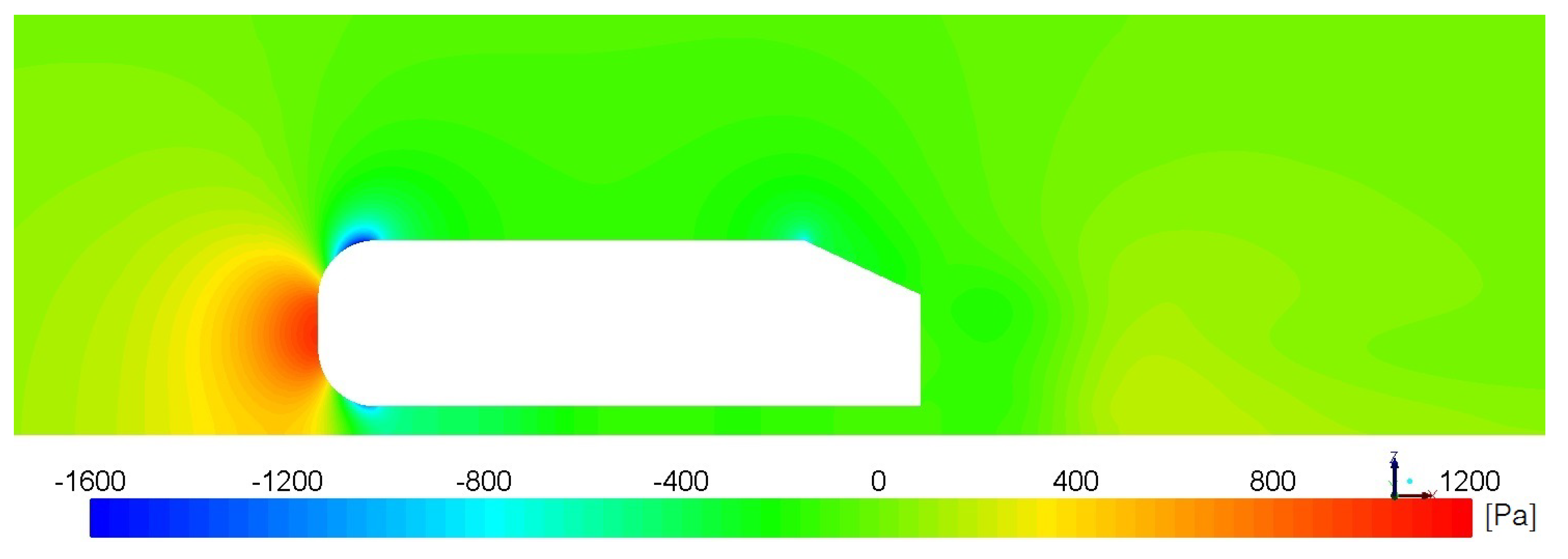
3.1. Velocity and Pressure Field in Symmetry Plane

As results of the steady-state simulation using the $k-\omega$ SST turbulence model, the pressure field (Figure 4) and velocity field (Figure 5 and Figure 6) were received. The results from the simulation are compared with studies by other authors. The similarity criteria are characteristic structures generated behind an Ahmed body (recirculation and edge vortices) and velocity profiles in the symmetry plane, as well as drag coefficients.

Figure 7 schematically shows the vortex structures: the separation bubble above the rear part of the vehicle, two recirculation bubbles behind the geometry, and the c-pillar vortex generated on the rear side edge of the Ahmed body. Similar structures were observed from the simulation in Figure 6 and Figure 8. Additionally in Figure 8 the results are presented in isometric view. Area A represent the separation bubble, areas B1, B2 are recirculation bubbles, and area C is the c-pillar vortex.

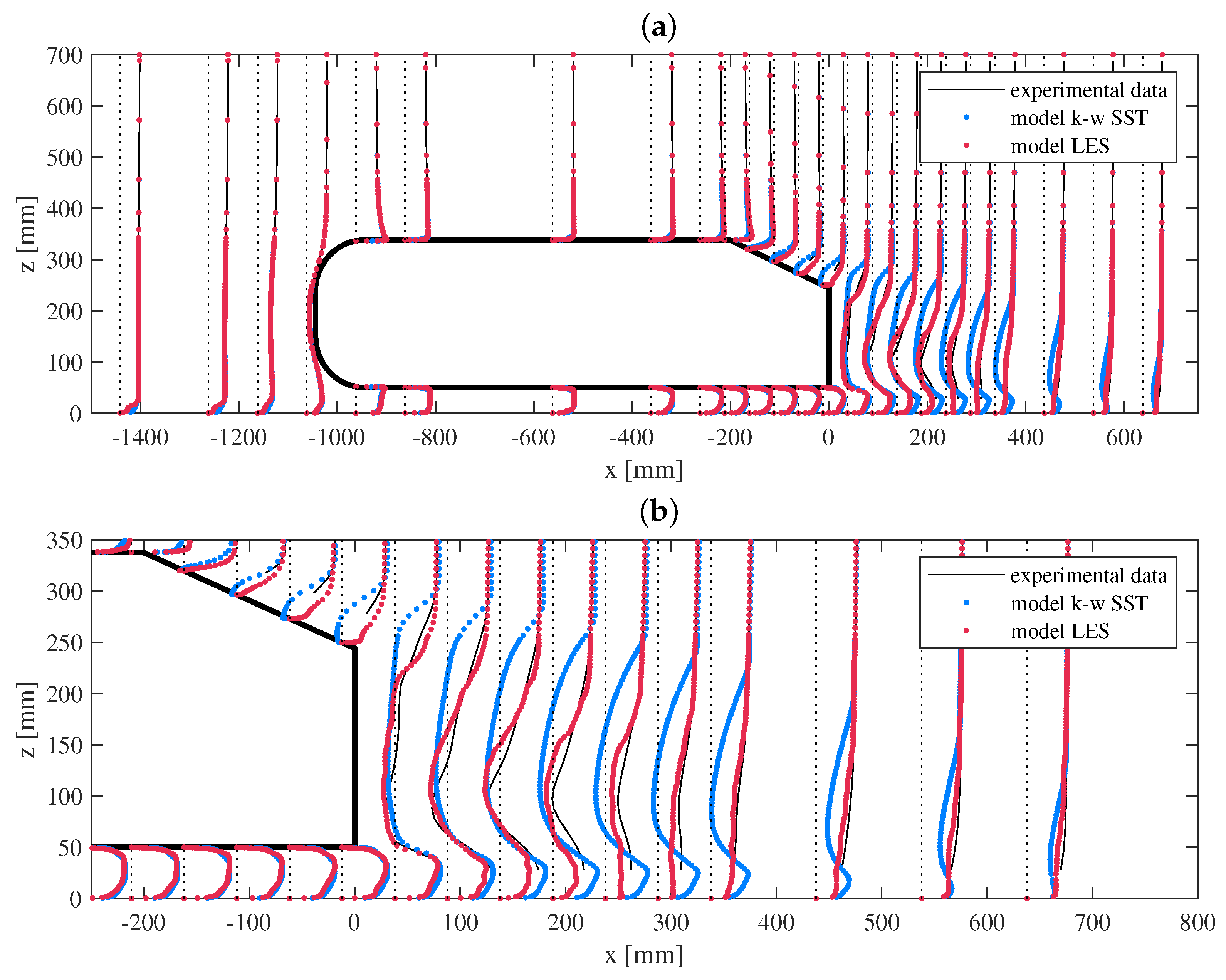
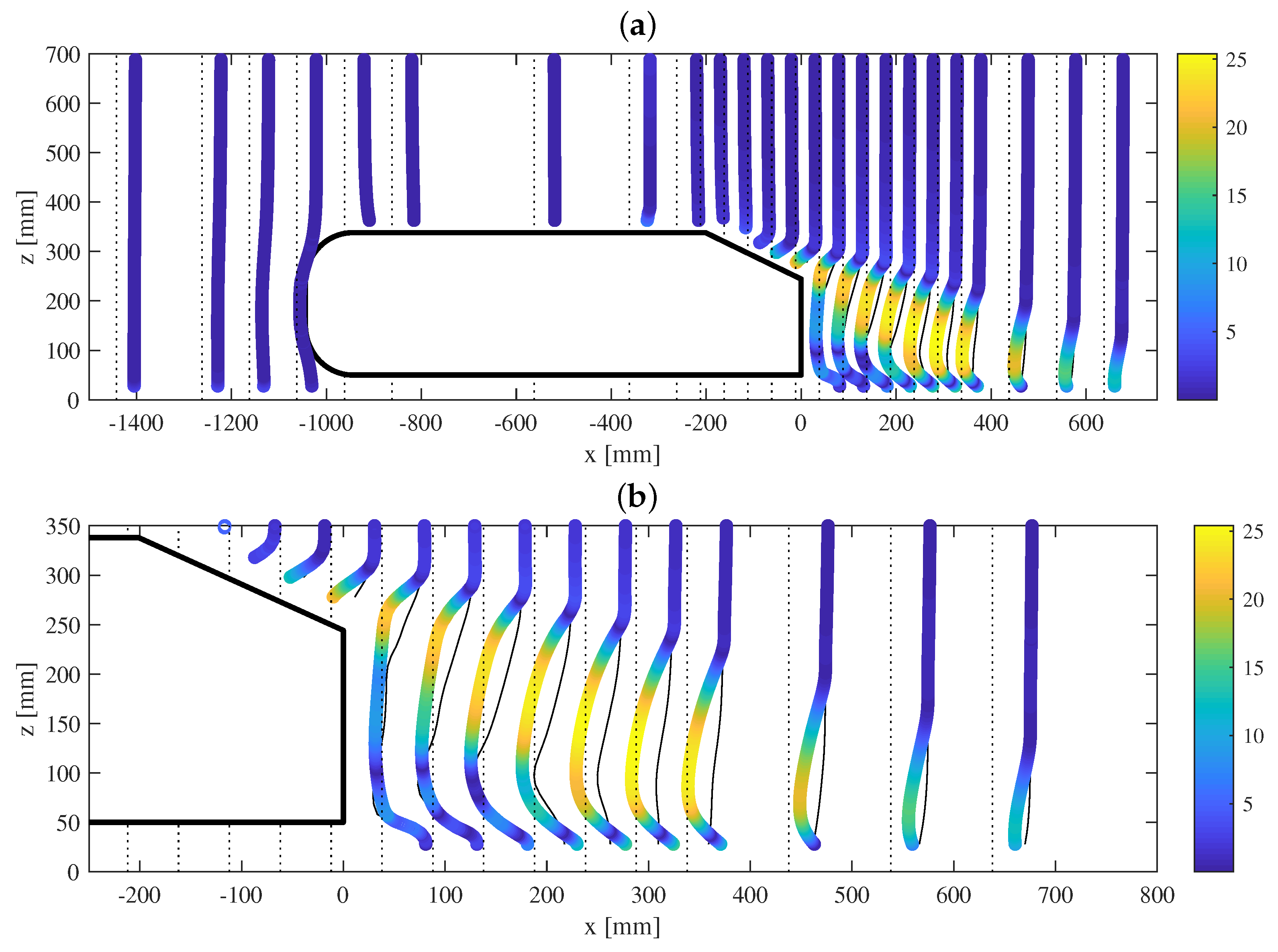
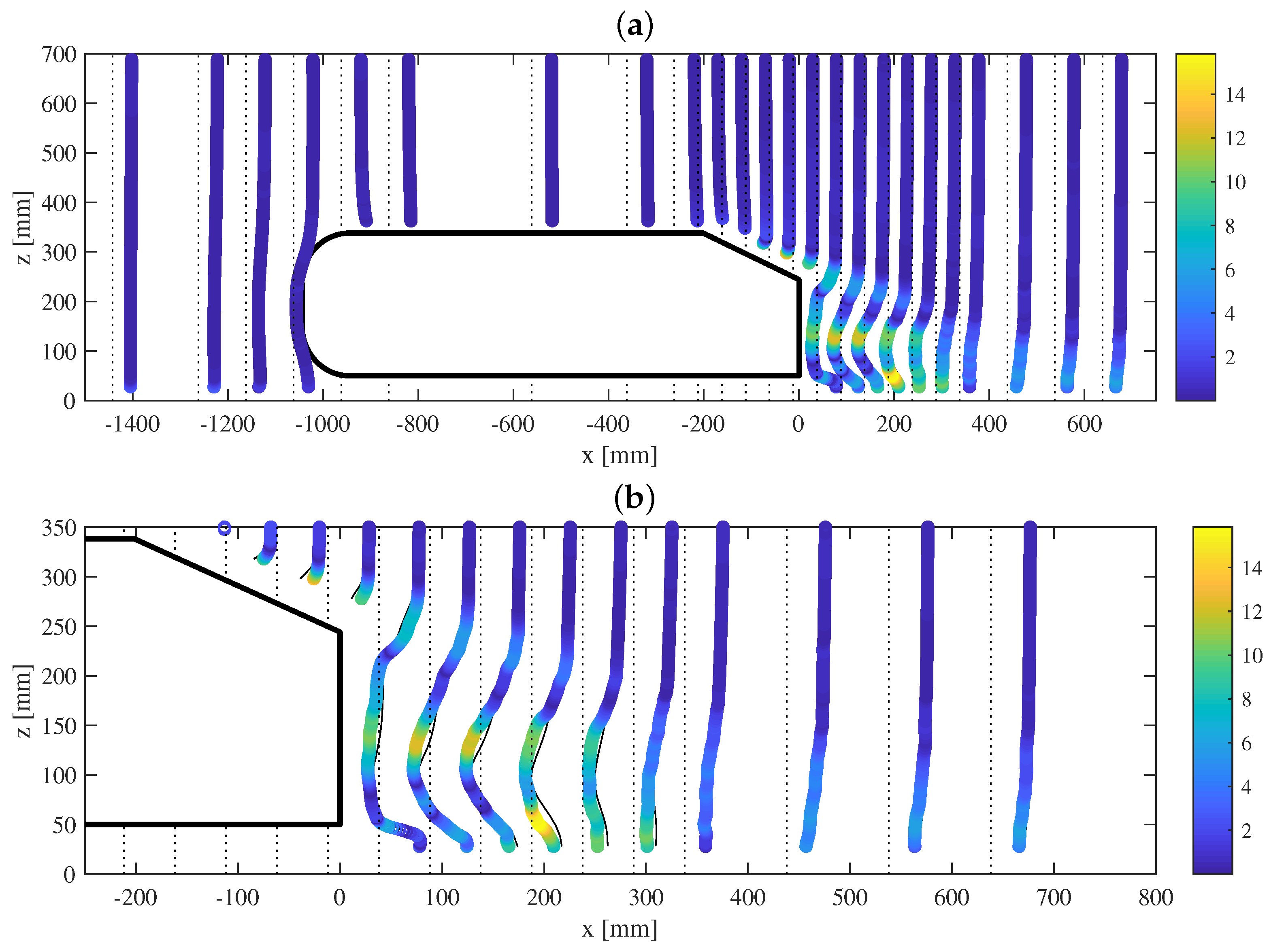
3.2. Steamwise Velocity Profile in Symmetry Plane

In order to compare results from the numerical simulation with the experiment, the streamwise velocity profile were used. The velocity profile shows velocity vectors for specific coordinates marked as a straight rake of black dots in Figure 9. The distance between a rake of black dots and the results is the value of the velocity vector in the x direction. Streamwise velocity profiles were compared around the reference geometry for two different turbulence models: the $k-\omega$ SST (blue rake of dots) and LES (red rake of dots). The air velocity was assumed as 40 m/s. The reference point for the simulation tests was the experimental data (black lines) available from Lienhart et al. [19].

The results received using the $k-\omega$ SST turbulence model allowed to map the velocity field very precisely, especially for the front and middle parts of the body. In the wake a deviation is observable from the experimental data.

Further calculation using the LES turbulence model allowed us to achieve a much improved map of the wake. The absolute errors in the x direction for the $k-\omega$ SST and LES turbulence models are shown in the Figure 10 and Figure 11. To facilitate the comparison of data, a velocity colormap is used. In order to compare results from the experiment with results from the LES unsteady turbulence model, the arithmetic average of the velocity was taken. The results from the simulation for the LES turbulence model were stored every 1305 time steps, where each time step was ${10}^{-5}$ s.

After ${10}^4$ iterations, the drag and lift coefficients were stable (Figure 12) and changing around the mean value. The streamwise velocities in that case were calculated as the average of the velocity results from the time band of 0.1 to 0.35 s.

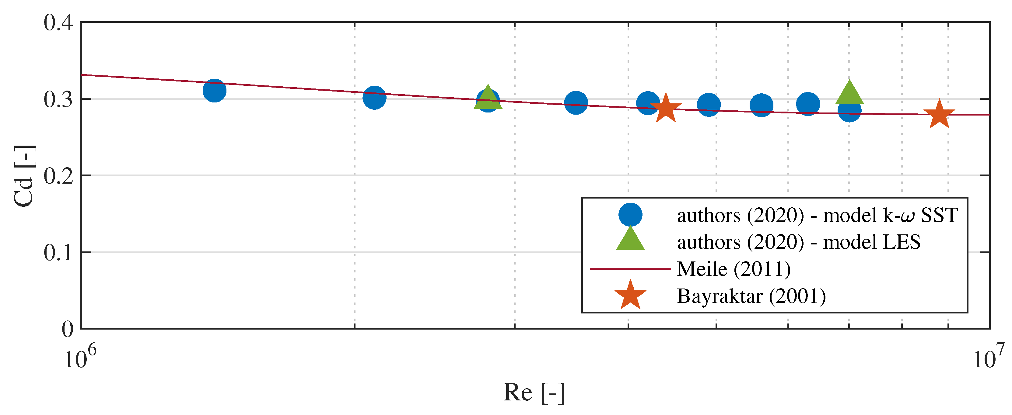
3.3. Drag Coefficient

Simulation studies were carried out for nine different speeds in the range from 20 to 100 m/s for the $k-\omega$ SST turbulence model and two different speeds, 40 and 100 m/s, for the LES turbulence model. The drag coefficients were compared with the results of other researchers [13,20] and presented as a function of the Reynolds number (Figure 13). The obtained relative error did not exceed 8.35% comparing to the Meile fit. For the aeroacoustic calculation the free stream velocity was 40 m/s. In that case the drag coefficient relative errors for the $k-\omega$ SST and LES turbulence models were 0.16 and 0.06%.

3.4. Sound Pressure Level (SPL)

Assuming windless weather conditions, the speed of the air relative to the road is zero. For this reason in everyday road situations the vehicle is a source of aerodynamic noise. However, in the case of the studied Ahmed body geometry it is quite different. We will use a numerical model with a reference structure to compare the simulation data with a future experimental study. Therefore two surfaces were chosen as the sources of sound in this model. The first is connected with the surface of the Ahmed body, which is irregular. The second is the bottom plane under the body. The generated pressure fluctuation was measured at the mid height of the Ahmed body core for the z-coordinate of 194 mm. Around the geometry 39 receivers were defined, which are shown in Figure 14. The receiver number is located at the center of the data point. The distances between receivers are 1, 2 and 4 m, except for receivers that are located close to the Ahmed body surface. The overall sound pressure level (OASPL) was calculated according to Equation (16) to one decimal place, where $p^{\prime }$ is substituted by the root mean square pressure fluctuation from the time range of 0.1 to 0.35 s. The results are also shown in Figure 14 but in a northwestern position from the data point. To facilitate analysis a colormap is used. Except for receivers located just next to the surface of the Ahmed body, the highest OASPL is observed in the wake, behind the geometry.

The A-weighting sound pressure level for three receivers, 12, 13, and 19, is presented in Figure 15. Points 12 and 13 are located behind the Ahmed body in an area of a high turbulence structure. Point 19 was chosen on the side in the distance of 1 m from the vehicle surface. Similar localization of receivers will be used in a future study, which will be concentrated on the emission of aerodynamic noise generated by a moving column of vehicles to the environment.

The highest values of A-weighting sound pressure levels were observed for low frequencies in the range from 180 to 1400 Hz in all three positions.

4. Discussion and Conclusions

In this work, numerical calculation was used in order to study an Ahmed body model. The purpose of the work was to build a numerical model using two turbulence models, $k-\omega$ SST and LES, as well as its verification based on experimental measurement data. The model quality was verified in two stages. The first stage was to prepare and ensure the good quality of the constructed computational mesh. The boundary layer was defined with a corresponding parameter y+, which was around 1. The growth ratio between the elements was set at 1.15. The minimum orthogonal quality parameter was 0.323, while the aspect ratio did not exceed 60. The second stage of the model verification consisted in comparing the simulation calculation with the experimental measurement data, as well as with the numerical results obtained by other authors. The main criterion adopted was the comparison of the streamwise velocity profiles in the symmetry plane and the drag coefficient $C_d$. In addition, the steady-state calculation confirmed the characteristic structures formed behind the vehicle model. The numerical model developed in the work, using the LES turbulence model, is of good quality. The two-stage research process related to the development of the model and the verification by experimental study allows to clearly state that the developed numerical model is correct. Further CAA analysis was possible using the FW-H analogy.

FFT analysis transformed pressure versus time characteristic to frequency domain. In order to reduce acoustic noise generated by the Ahmed body geometry it is important to eliminate high values of sound pressure levels from the frequency range of 180 to 1400 Hz.

The introduced methodology of using a colormap to compare of results of velocity profiles simplified the analysis of troubling areas of the calculation grid. For further analysis using the $k-\omega$ SST turbulence model the mesh in the wake area should be improved. In case of using the LES turbulence model the absolute velocity error was partly the result of the method used to average the results every 1305 time steps.

When analyzing the drag coefficient in respect to other studies, the biggest relative errors were observed for higher velocities, especially for the LES turbulence model. This kind of problem could be related with insufficient quality and density of the mesh. One possible solution would be using adaptive mesh refinement for automatically increasing the density in high turbulence areas [21].

Computing the steady-state flow using the $k-\omega$ SST turbulence model and the setting results from this simulation as initial conditions for transient simulation was a useful method to reduce computation time. However, in order to evaluate computational resource reduction further calculation is needed.

The study on an aeroacoustic numerical model of an Ahmed body was performed as part of a calculation grant in CYFRONET on the computing cluster PROMETHEUS. The total used walltime exceeded 60,000 h, where the number of cores reached up to 24 for a single simulation. ANSYS Fluent software was used as a solver. Further calculations and visualizations of the results were made in MATLAB software.

Created an aeroacoustic model of the Ahmed body will be used in a future study on aerodynamic and acoustic phenomena connected with a moving column of vehicles.

References

1. Helfer, M. General Aspects of Vehicle Aeroacoustics. In Proceedings of the Lecture Series on Road Vehicle Aerodynamics, Sint-Genesius-Rode, Belgium, 30 May–3 June 2005. [Google Scholar]
2. Shi, X.; Sun, D.J.; Fu, S.; Zhao, Z.; Liu, J. Assessing On-Road Emission Flow Pattern under Car-Following Induced Turbulence Using Computational Fluid Dynamics (CFD) Numerical Simulation. Sustainability 2019, 11, 6705. [Google Scholar] [CrossRef] [Green Version]
3. Żółtowski, P.; Piechna, J.; Żółtowski, K.; Zobel, H. Analysis of dynamic loads on lightweight footbridge caused by lorry passing underneath. Bull. Pol. Acad. Sci. Tech. Sci. 2006, 54, 33–43. [Google Scholar]
4. Ahmet, A.; Tahsin, E.; Halit, Y.; Alper, Y.; Ahmet, H.P. Computational Fluid Dynamics Analysis of a Vehicle Radiator Using Porous Media Approach. Heat Transf. Eng. 2020, 1–13. [Google Scholar] [CrossRef]
5. Mo, J.O.; Choi, J.H. Numerical investigation of unsteady flow and aerodynamic noise characteristics of an automotive axial cooling fan. Appl. Sci. 2020, 10, 5432. [Google Scholar] [CrossRef]
6. Bergamini, P.; Casella, M.; Vitali, D.F. Computational Prediction of Vehicle Aerodynamic Noise by Integration of a CFD Technique with Lighthill’s Acoustic Analogy. SAE Int. 1997. [Google Scholar] [CrossRef]
7. Tsai, C.-H.; Fu, L.-M.; Tai, C.-H.; Huang, Y.-L.; Leong, J.-C. Computational aero-acoustic analysis of a passenger car with a rear spoiler. Appl. Math. Model. 2009, 33, 3661–3673. [Google Scholar] [CrossRef]
8. Duncan, B.D.; Sengupta, R.; Mallick, S.; Shock, R.; Sims-Williams, D.B. Numerical Simulation and Spectral Analysis of Pressure Fluctuations in Vehicle Aerodynamic Noise Generation. SAE Int. J. Passeng. Cars Mech. Syst. 2002, 111, 872–892. [Google Scholar]
9. Ahmed, S.R.; Ramm, G.; Faltin, G. Some Salient Features Of The Time-Averaged Ground Vehicle Wake. SAE Int. 1984, 473–503. [Google Scholar] [CrossRef]
10. Guilmineau, E.; Deng, G.B.; Leroyer, A.; Queutey, P.; Visonneau, M.; Wackers, J. Assessment of hybrid RANS-LES formulations for flow simulation around the Ahmed body. Comput. Fluids 2017, 176, 302–319. [Google Scholar] [CrossRef]
11. Serre, E.; Minguez, M.; Pasquetti, R.; Guilmineau, E.; Deng, G.B.; Kornhaas, M.; Schäfer, M.; Fröhlich, J.; Hinterberger, C.; Rodi, W. On simulating the turbulent flow around the Ahmed body: A French–German collaborative evaluation of LES and DES. Comput. Fluids 2013, 78, 10–23. [Google Scholar] [CrossRef]
12. Banga, S.; Zunaid, M.; Ansari, N.A.; Sharma, S.; Dungriyal, R.S. CFD Simulation of Flow around External Vehicle: Ahmed Body. IOSR J. Mech. Civ. Eng. 2015, 12, 87–94. [Google Scholar] [CrossRef]
13. Meile, W.; Brenn, G.; Reppenhagen, A.; Lechner, B.; Fuchs, A. Experiments and numerical simulations on the aerodynamics of the Ahmed body. CFD Lett. 2011, 3, 32–39. [Google Scholar]
14. Thomas, B.; Agarwal, R.K. Evaluation of Various RANS Turbulence Models for Predicting the Drag on an Ahmed Body. In Proceedings of the AIAA Aviation Forum, Dallas, TX, USA, 17–21 June 2019. [Google Scholar]
15. Han, X.; Rahman, M.M.; Agarwal, R.K. Development and Application of a Wall Distance Free Wray-Agarwal Turbulence Model. In Proceedings of the AIAA SciTech Forum, Kissimmee, FA, USA, 8–12 January 2018. [Google Scholar]
16. Dykas, S.; Wróblewski, W.; Rulik, S.; Chmielniak, T. Numerical Method for Modeling of Acoustic Waves Propagation. Arch. Acoust. 2010, 35, 35–48. [Google Scholar] [CrossRef] [Green Version]
17. Sosnowski, M. The influence of computational domain discretization on CFD results concerning aerodynamics of a vehicle. J. Appl. Math. Comput. Mech. 2018, 17, 79–88. [Google Scholar] [CrossRef]
18. Mansour, M.; Khot, P.; Kováts, P.; Thévenin, D.; Zähringer, K.; Janiga, G. Impact of computational domain discretization and gradient limiters on CFD results concerning liquid mixing in a helical pipe. Chem. Eng. J. 2020, 383, 123121. [Google Scholar] [CrossRef]
19. Lienhart, H.; Becker, S.; Stoots, C. Flow and Turbulence Structures in the Wake of a Simplified Car Model (Ahmed Model). Notes Numer. Fluid Mech. 2002, 77, 1–8. [Google Scholar]
20. Bayraktar, I.; Landman, D.; Baysal, O. Experimental and Computational Investigation of Ahmed Body for Ground Vehicle Aerodynamics. SAE Int. 2001, 321–331. [Google Scholar] [CrossRef] [Green Version]
21. Murawski, K.; Lee, D. Numerical methods of solving equations of hydrodynamics from perspectives of the code FLASH. Bull. Pol. Acad. Sci. 2011, 59, 81–91. [Google Scholar] [CrossRef] [Green Version]
Figure 1. Dimensions of the Ahmed body used in this paper.
Applsci 10 09066 g001
Figure 2. 3D hexahedral mesh around the Ahmed body. Grid for 5.1 million elements.
Applsci 10 09066 g002
Figure 3. Surface description for boundary conditions.
Applsci 10 09066 g003
Figure 4. Pressure distribution around the Ahmed body at symmetry plane.
Applsci 10 09066 g004
Figure 5. Velocity distribution around the Ahmed body at the symmetry plane.
Applsci 10 09066 g005
Figure 6. Streamlines around the Ahmed body at symmetry plane.
Applsci 10 09066 g006
Figure 7. Vortex system in wake (schematic) [9].
Applsci 10 09066 g007
Figure 8. Vortex system in wake (simulation).
Applsci 10 09066 g008
Figure 9. Streamwise velocity profiles in the symmetry plane y = 0 . Black lines for experimental data, blue dots for model k ω SST, red dots for model LES. (a) General view; (b) zoom at the back of the Ahmed body.
Applsci 10 09066 g009
Figure 10. Velocity error for the k ω SST turbulence model. Experimental data are presented as black lines. The unit of the colormap is meter per second (m/s). (a) General view; (b) zoom at the back of the Ahmed body.
Applsci 10 09066 g010
Figure 11. Velocity error for the LES turbulence model. Experimental data are presented as black lines. The unit of the colormap is meter per second (m/s). (a) General view; (b) zoom at the back of the Ahmed body.
Applsci 10 09066 g011
Figure 12. Drag and lift coefficients as a function of time for the LES turbulence model.
Applsci 10 09066 g012
Figure 13. Drag coefficient (Cd) as a function of Reynolds number (Re).
Applsci 10 09066 g013
Figure 14. Overall sound pressure level in decibels (dBs) around the Ahmed body, measured at receivers for the z-coordinate of 194 mm. View from the top.
Applsci 10 09066 g014
Figure 15. A-weighting sound pressure level provided by terce for receivers 12, 13, and 19.
Applsci 10 09066 g015