Abstract
Noise pollution is one of the major urban environmental pollutions, and it is increasingly becoming a matter of crucial public concern. Monitoring and predicting environmental noise are of great significance for the prevention and control of noise pollution. With the advent of the Internet of Things (IoT) technology, urban noise monitoring is emerging in the direction of a small interval, long time, and large data amount, which is difficult to model and predict with traditional methods. In this study, an IoT-based noise monitoring system was deployed to acquire the environmental noise data, and a two-layer long short-term memory (LSTM) network was proposed for the prediction of environmental noise under the condition of large data volume. The optimal hyperparameters were selected through testing, and the raw data sets were processed. The urban environmental noise was predicted at time intervals of 1 s, 1 min, 10 min, and 30 min, and their performances were compared with three classic predictive models: random walk (RW), stacked autoencoder (SAE), and support vector machine (SVM). The proposed model outperforms the other three existing classic methods. The time interval of the data set has a close connection with the performance of all models. The results revealed that the LSTM network could reflect changes in noise levels within one day and has good prediction accuracy. Impacts of monitoring point location on prediction results and recommendations for environmental noise management were also discussed in this paper.
1. Introduction
The Internet of Things (IoT) is an idea that connects the physical objects to the Internet, which can play a remarkable role and improve the quality of our lives in many different domains [1,2]. There are many possibilities and uncertainties in the application scenarios of IoT [3]. The application of the IoT in the urban area is of particular interest, as it facilitates the appropriate use of the public resources, enhancing the quality of the services provided to the citizens, and minimizing the operational costs of the public administrations, thus realizing the Smart City concept [4]. The urban IoT may provide a distributed database collected by different sensors to have a complete characterization of the environmental conditions [2]. Specifically, urban IoT can provide noise monitoring services to measure the noise levels generated at a given time in the places where the service is adopted [5].
With the unprecedented rate of urbanization as a result of the rapid acceleration of economic and population growth, new problems arose, such as traffic congestion, waste management, pollution, and parking allocation [6]. Recently, noise pollution has become one of the core urban environmental pollutions and has received increasing attention. Urban noise pollution can cause various consequences, especially severe effects on human health such as hearing damage, affecting sleep and increasing psychological stress [7,8]. To solve the problem of noise pollution, the Chinese government issued the Law on the Prevention and Control of Environmental Noise Pollution of the People’s Republic of China [9] and adopted a series of policy measures on controlling urban noise, rural noise, industrial noise, construction noise, etc. However, due to the variety of noise sources [10] and the prevalence of noise pollution, the problem of environmental noise pollution in China has not been adequately solved and remained as one of the main urban ecological problems. The Chinese Environmental Noise Pollution Prevention Report showed that in 2017, environmental noise-related complaints received by environmental protection departments at all levels accounted for 42.9% of the total environmental complaints [11]. According to the latest release of the Beijing–Tianjin–Hebei research report of the environmental resource based on the big data analysis in June 2018, noise pollution cases accounted for 73% of the total number of cases in the Beijing–Tianjin–Hebei regional environmental pollution case [12]. Therefore, paying attention to urban environmental noise pollution and making an accurate and timely prediction of environmental noise will assist in comprehensively grasping and managing the urban acoustic environment, thus improving residents’ life satisfaction.
Noise prediction has significant theoretical research value and practical significance. In past studies, the authors proposed many methodologies to evaluate and predict the noise in the environment. These prediction methods are mainly classified into three groups: physical propagation models, traditional statistical methods, and machine learning methods.
The first group of noise prediction methods is the physical propagation model, which predicts the ambient noise of another location from the spatial perspective, based on the distance from the sound source to the calculated noise location point and the physical properties of the sound source itself. Since the early 1960s, many developed countries conducted research on airport noise and introduced many airport noise management methods and models [13,14], such as the Integrated Noise Model promoted by the Federal Aviation Authority, the Aircraft Noise Contour (ANCON) model of the United Kingdom and the Fluglaerm (FLULA) program developed in Switzerland [15,16,17]. Some studies focused on the spatial propagation of noise to predict environmental noise [18,19]. For example, based on the propagation model of noise attenuation, the noise distribution can be drawn [20]. There are also studies on choosing the location of noise monitoring sites to make the monitoring more effective [21]. In general, there are few studies focusing on the temporal variation of urban noise using physical propagation models [18,19,20,21].
The second group of noise prediction methods is the traditional statistical method. Kumar and Jain [22] proposed an autoregressive integrated moving average (ARIMA) model to predict traffic noise time series, but the amount of data was small, and the monitoring time was only a few hours. It is also concluded that it is better to consider the time series on a longer time scale. Garg et al. [23] analyzed the long-term noise monitoring data through ARIMA modeling technology and found that the ARIMA method is reliable for time series modeling of traffic noise, but the corresponding parameters should be adjusted according to different situations. Gajardo et al. [24] performed a Fourier analysis of the traffic noise of the two cities of Cáceres and Talca, and discovered that regardless of the measurement environment of the city and the corresponding traffic flow, larger periodic components and amplitude values are similar in different samples, which indicated that urban traffic noise has an inherent law that can be predicted. There is also a study that developed models based on the regression model to prognosticate the level of noise in closed industrial spaces through the dominant frequency cutoff point [25].
The third group of noise prediction methods is the machine learning method. Rahmani et al. [26] introduced the genetic algorithm into the traffic noise prediction and proposed two prediction models, and the simulation on the actual data achieved an accuracy of ±1%. Wang et al. [27] occupied a back propagation neural network to simulate traffic noise. Iannace et al. [28] used a random forest regression method to predict wind turbine noise. Torija and Ruiz [29] used the feature extraction and machine learning methods to predict the environmental noise and got an excellent fitting effect. However, the number of input variables was 32, the distinction is subtle, and it is challenging to organize the data.
The prediction of environmental noise heavily depends on historical and real-time noise monitoring data. The research by Frank et al. [30] shows that combining the rules or patterns mined in the monitoring data with the acoustic theoretical calculation model can effectively improve the prediction accuracy of noise. In terms of reflecting regional noise levels, sometimes sampling strategies are put forward based on considerations of saving resources and improving data acquisition efficiency [31]. Giovanni et al. [32] found that considering saving the time cost and the accuracy of the results, a non-continuous 5–7 days observation of noise is reasonable for long-term noise prediction.
Forecasting the temporal variation of noise can offer a scientific basis for urban noise control. In recent years, with the widespread utilization of sound level meters and the development of various sensor network technologies, environmental noise data has an exploding expansion. Although there have been previous studies on noise measurement, prediction, and control [19,22,23,25,33,34,35,36], most of the research data are relatively diminutive. This gave the inspiration to have a second thought about the environmental noise prediction problem, that is, whether there are more optimized noise prediction models and methods when handling an abundant amount of noise data. Therefore, predicting noise in the time dimension requires a more efficient approach. However, at a fine time interval, few studies have focused on and predicted the variation of noise within a given day so far.
Deep learning has developed rapidly and has been successfully applied in many specialties lately [37]. It utilizes multiple-layer architectures or deep architectures to extract inherent features in data from the lowest level to the highest level, and they can discover huge amounts of structure in the data [38]. Deep learning is derived from the study of artificial neural networks. The most common neural network models include multilayer perceptron (MLP), convolutional neural networks (CNN), recurrent neural networks (RNN), etc. [39]. For time series, RNN is often employed to characterize the association of hidden states and capture the data characteristics of the entire sequence. Nevertheless, simple RNN has long-term dependence problems and cannot effectively utilize long-interval historical information. Therefore, long short-term memory (LSTM) network has emerged to unravel the problem of gradient disappearance, which has been used for stock price forecasting [40], air quality forecasting, sea surface temperature forecasting [41], flight passenger number forecasting, and speech recognition [42]. The results illustrated that the model had achieved excellent performance.
In this study, we deployed an IoT-based noise monitoring system to acquire the urban environmental noise, and proposed an LSTM network to predict the noise at different time intervals. The performance of the model was compared with three classic predictive models—random walk (RW), stacked autoencoder (SAE), and support vector machine (SVM) on the same dataset. This study also explored the impact of monitoring point location on prediction results and policy recommendations for environmental noise management.
2. Materials and Methods
2.1. Urban Environmental Noise Monitoring Based on IoT
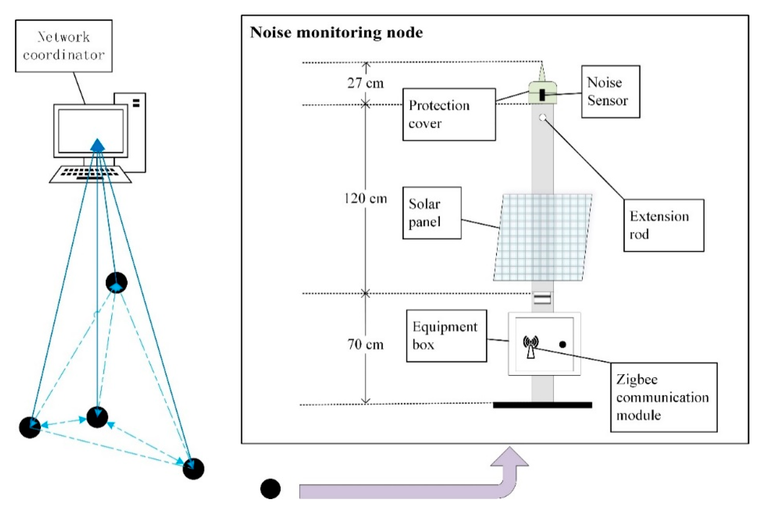
IoT systems offer environmental and ecological monitoring [3]. In this study, we deployed an IoT-based noise monitoring system powered by solar panels, as depicted in Figure 1. The system uses the HS5633T sound level meter following the Chinese GB/T 3785 standard of noise measurement, with the microphone placed at 1.90 m from the floor, and the IP-Link2220H wireless communication modules for data transmission. The noise data monitored by the noise sensors are transmitted back to the network coordinator for storage by the Zigbee wireless protocol. Due to the relatively small number of nodes, a mesh network structure was employed to enhance the efficiency of communication. The data was received and stored using noise-receiving software developed by the authors and Lenovo Thinkpad laptop server hardware.
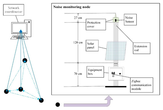
Figure 1.
Noise monitoring system based on IoT.
2.2. LSTM Recurrent Neural Network
The traditional recurrent neural network (RNN) can pass the previous information to the current task, but when the distance between the related information and the required information is considerable, the RNN becomes unable to connect the relevant information [43]. In order to learn the long-distance dependency problem, Hochreiter and Schmidhuber [44] proposed the LSTM network, and it has been improved and promoted by some scholars [45,46]. LSTM avoids long-term dependency problems through an explicit design. It is practically the default behavior of LSTM to remember the long-term information.
The LSTM network replaces the neurons in the RNN with the LSTM unit, and adds input gates, output gates, and forget gates to input, output, and forget past information to control how much information can pass (Figure 2) [47]. LSTM has two transmission states namely, a cell state, and a hidden state. The state of the cell changes slowly with time, and the hidden state at different times may be different. LSTM establishes a gate mechanism to achieve the trade-off between the previous input and the current input. The main essence is to adjust the focus of memory according to the training goal and then perform the whole series of coding. LSTM can alleviate the vanishing gradient problem, exploding gradient problem of RNN, and performs favorably than RNN on longer sequences [44,48].
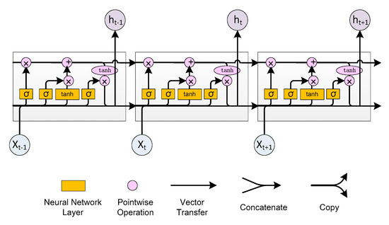
Figure 2.
LSTM architecture with one memory block.
The LSTM has a “gate” structure to remove or add information to the cell state. A gate is a method of selectively passing information, including a sigmoid neural network layer and a bitwise multiplication operation [44]. The LSTM workflow and mathematical representation mainly have the following four steps [47]:
- (1)
- Deciding to discard information:
This step is implemented by a forgetting gate that outputs a value between 0–1 to by reading and , “0” means completely discarded, and “1” indicates complete retention.
- (2)
- Determining updated information:
This step determines what new information is stored in the cell state and consists of two parts, the first part is the sigmoid layer (the input gate), to ascertain which value is to be updated, while the second part is a new candidate value created by a tanh layer.
- (3)
- Updating the cell status:
This step is implemented by updating the state of the old cell, multiplying the old state by , discarding the information to be forgotten, and adding to obtain a new candidate value.
- (4)
- Outputting information:
This step determines the final output. Firstly, a sigmoid layer determines which part of the cell state will be output, represented by . Secondly, the cell state is processed by the tanh function and multiplied by the output of the sigmoid layer to produce the output.
2.3. Proposed LSTM Model Framework
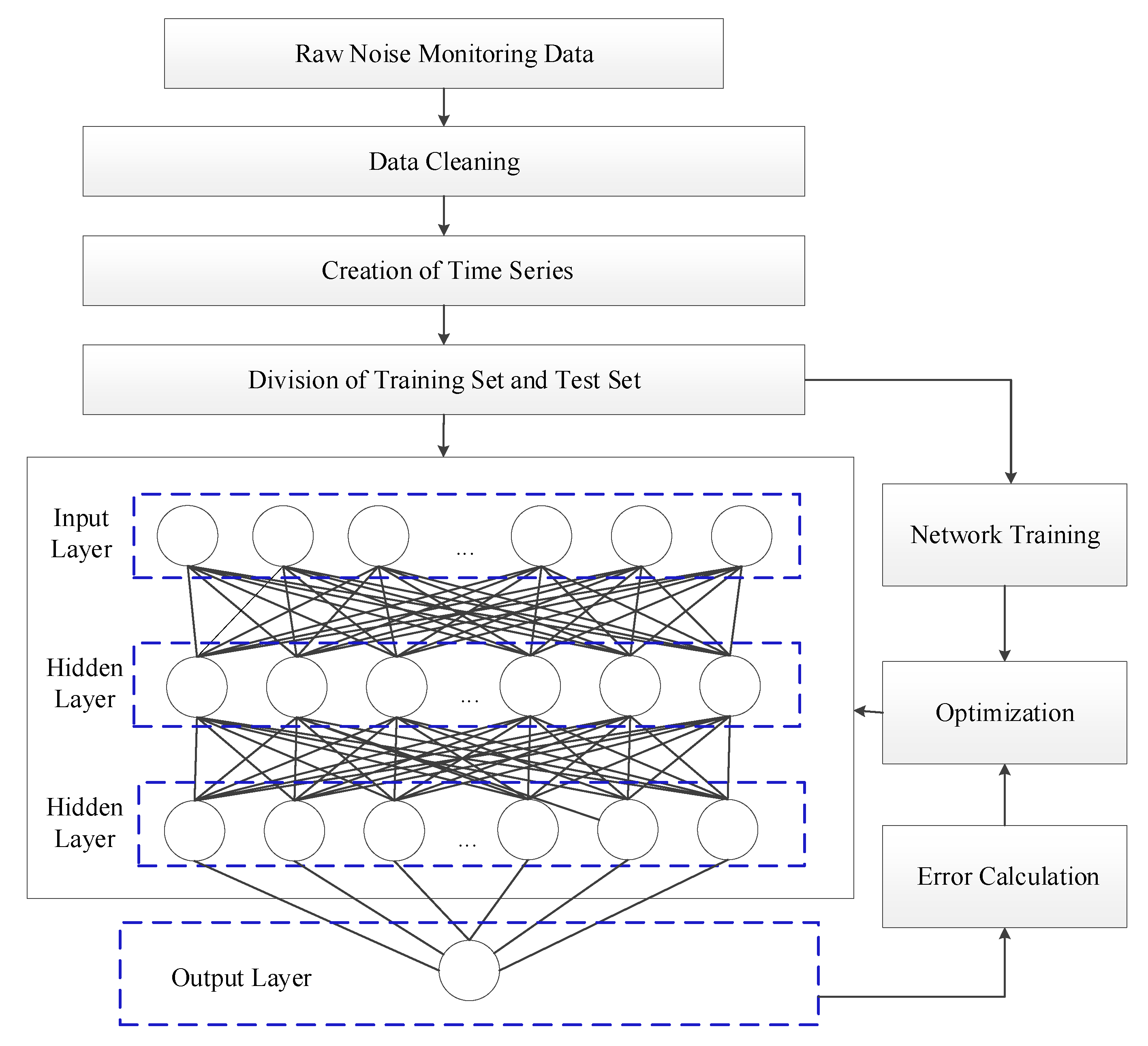
IoT must overcome some challenges to extract new insights from data [49]. In previous studies [18,19,20,21,22,23,24,25,26,27,28,29,30,31,32,33,34,35,36], environmental noise prediction mainly focused on the spatial propagation of noise, and there were few studies focused on the variation of noise in short-term. The noise data set used in this study is in seconds, which is more random. In view of the aforementioned situations, we proposed an LSTM-based environmental noise time series model, which includes an input layer, two hidden layers, and one output layer. The overall framework of the proposed LSTM model is depicted in Figure 3. The details on data cleaning, time series creation, and division of training set and test set are explained in the subsequent Section 3.2 and Section 3.4.
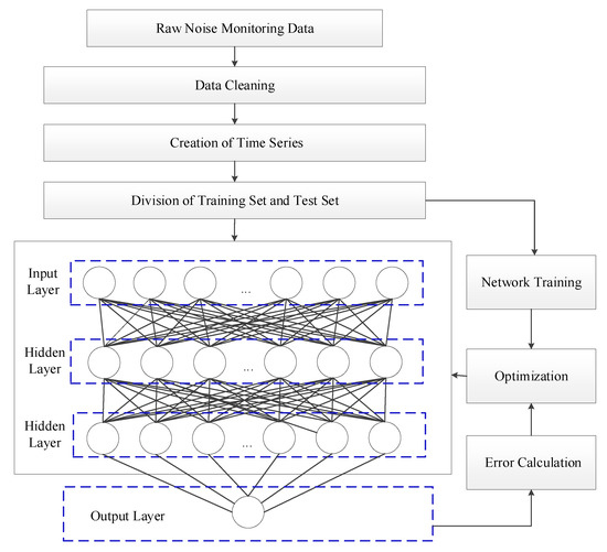
Figure 3.
Overall framework of the LSTM model.
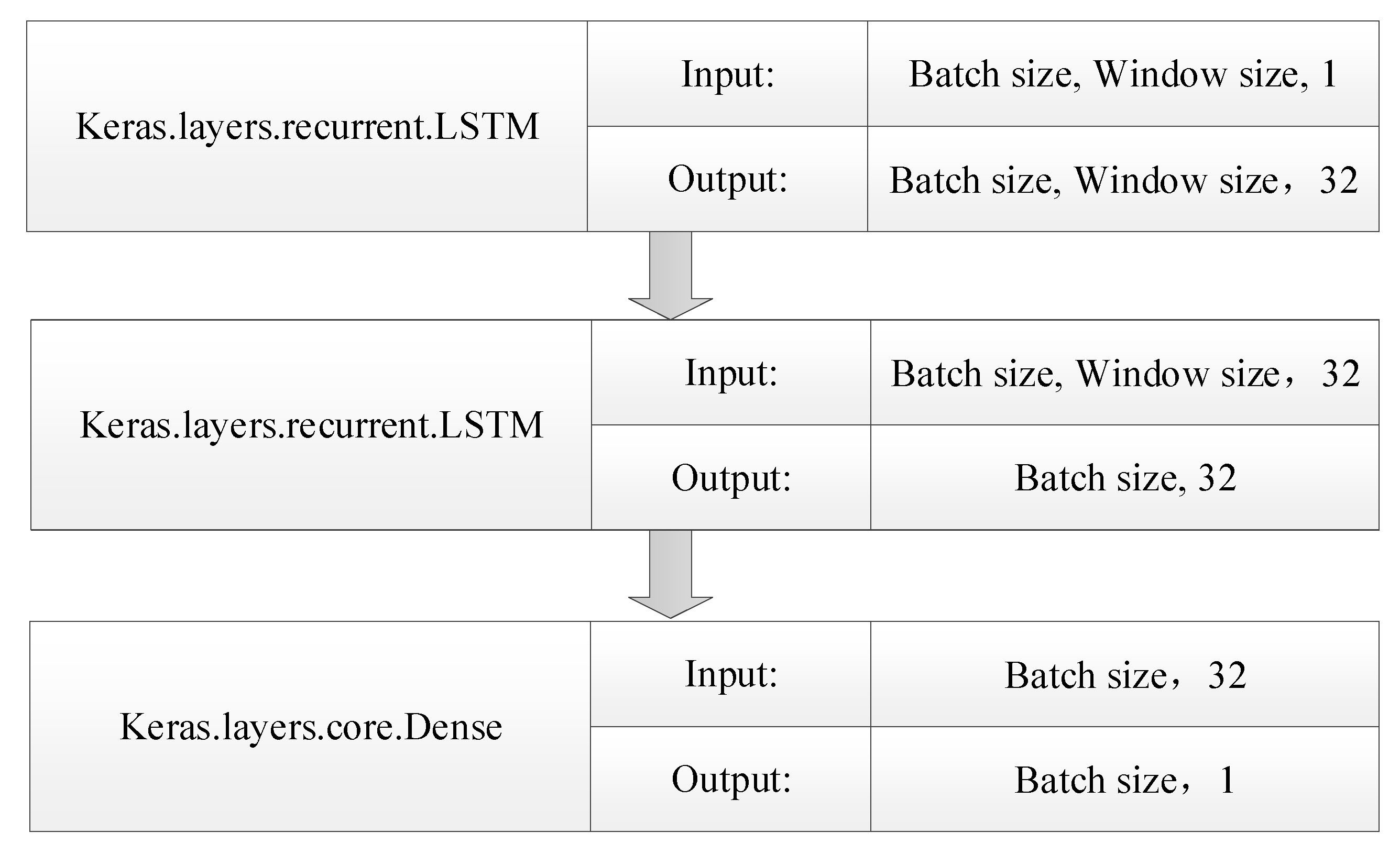
The model is put into operation with the aid of the deep learning framework Keras. The data flow form on each network layer is portrayed in Figure 4. The input is a three-dimensional tensor. As is depicted in Figure 4, the three-dimensional tensor consists of the batch size, the window size, and a number, which represents the number of input samples, the length of the time series, and the output dimension, respectively.
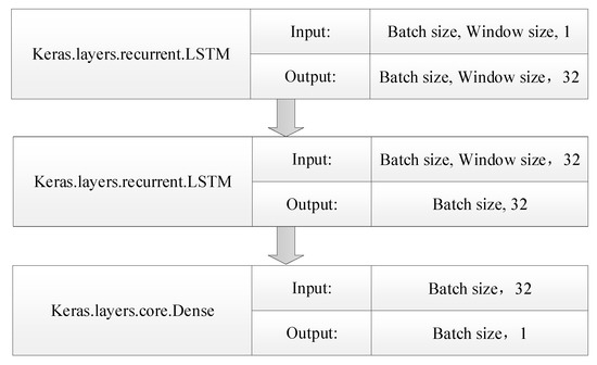
Figure 4.
Data flow on the network layer.
2.4. Network Configuration and Training
The root mean square error (RMSE) and the mean absolute error (MAE) are selected as the evaluation criteria for the performance of the model. The calculation formulas are
where represents the length of the test sequence, is the actual observation, is the predicted value, and smaller RMSE and MAE represent better prediction accuracy of the model.
Determining critical hyperparameters is significant in building a short-term noise prediction model based on LSTM [50]. According to the study by Greff et al., the interaction of hyperparameters in LSTM is minute [51], which means that each hyperparameter can be independently adjusted. The purpose of the tuning is to find the right parameters, rather than producing the final model. Generally, parameters that perform well on small data sets also perform satisfactorily on large data sets. To enhance the speed of the parameter adjustment, we used a streamlined data set, that is, the 1-min time interval was applied to average the noise monitoring data per minute, thereby compressing the length of the noise time series to 1/60 of the original.
Learning rate, number of hidden layer neurons, batch size and dropout are critical parameters of the model. 80% of the data is used as a training set, and 20% of the data is used as a test set in this study. In the network configuration process, only RMSE is used to evaluate the performance of the model.
The learning rate η has an essential influence on the performance of the model and is a relatively important parameter in the model. This study uses the hyperparameter optimization algorithm to optimize the learning rate. The commonly used adaptive learning rate optimization algorithms are AdaGrad, RMSProp, Adam, etc. [52]. Among them is the Adam algorithm, which combines the advantages of Adagrad to deal with sparse gradients and RMSprop to deal with non-stationary targets. It has little memory requirement and can calculate different adaptive learning rates for different parameters. Adam is best suited for most extensive data sets, high-dimensional spaces, and the most frequently used optimization algorithm [53]. Table 1 lists the model’s performance when using different optimization algorithms. As presented in Table 1, the performance of the Adam algorithm and Adadelta algorithm is similar, and the Adam algorithm is slightly better.

Table 1.
Model’s performance when using different optimization algorithms/dB(A).
Subsequently, the parameters are initialized to sequence length of 60, the number of neurons (neurons) of 32, and a batch size of 48. The number of iterations is 40. Then each hyperparameter was changed independently, and each test was repeated ten times. The average performance of the model in the training set and the test set is shown in Table 2. It was finally determined that the optimal number of hidden neurons was 64, the batch size was 126, and the dropout was 0.5.

Table 2.
Effect of different parameter settings on model fitting effect/dB(A).
3. Simulation Studies and Results
3.1. Data Preparation
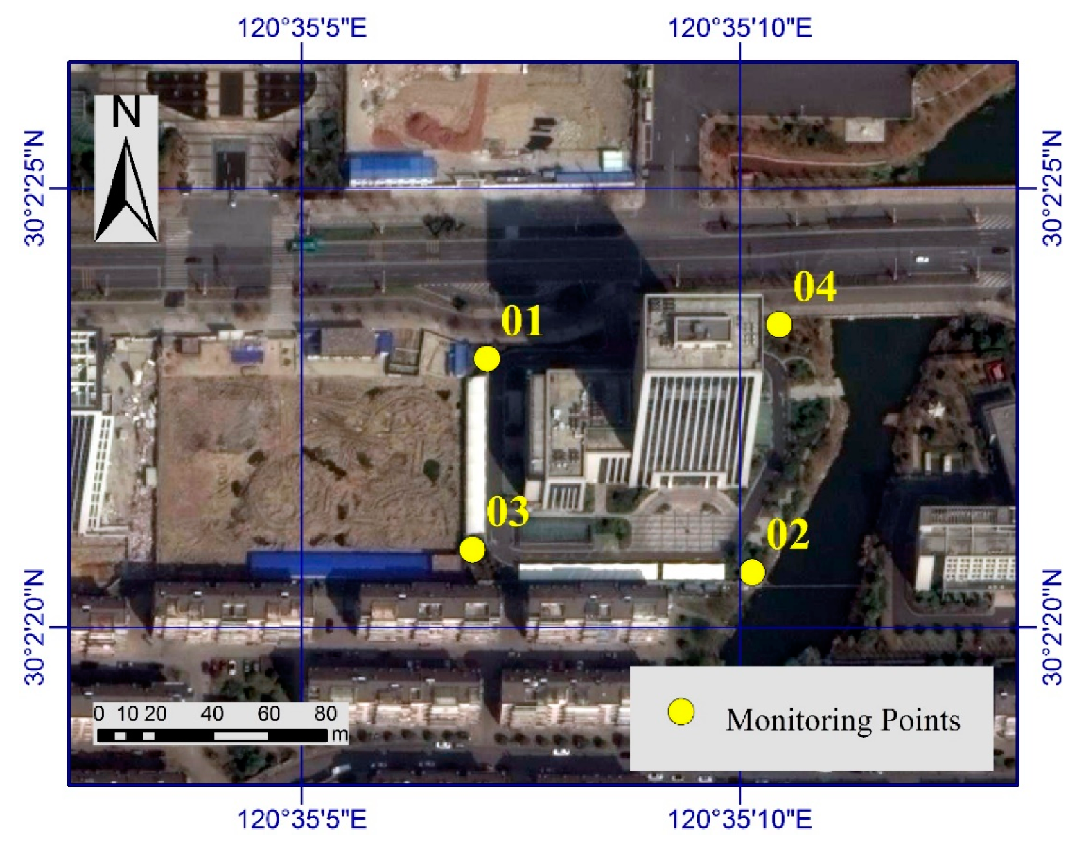
In this study, the data was acquired using an IoT-based noise monitoring system [54]. Shaoxing is located in the central northern part of Zhejiang Province and is among the key developing areas in China’s coastal economic zone. In this study, four sets of the system were installed in an administrative district of Shaoxing City, and the data acquisition interval was 1 s. Figure 5 shows the distribution of monitoring points (01, 02, 03, and 04). Point 01 is adjacent to a construction site and the main road. The primary noise sources are construction noise and traffic noise. Point 02 is near a small water surface (a river about 25 m wide) and a residential area, which means that in general, the noise level that can be monitored at this point is low. Point 03 is situated at a construction site and a residential area. The primary noise sources are construction noise and residential noise. Point 04 is close to the main road, and the primary noise source is traffic noise. The basic situation of noise monitoring points is represented in Table 3.

Figure 5.
Distribution of monitoring points.

Table 3.
Basic situation of monitoring points.
According to China’s technical specifications for the division of acoustic environment functional zones, the monitoring points are located in the administrative district types belonging to the same acoustic environment functional zones, and there are some comparabilities in urban functions and urban land types. The continuous 24-h noise monitoring was carried out in Shaoxing on August 15–21 (monitoring period a) and September 15–21 in 2015 (monitoring period b). After eliminating the null value, a total of 3,592,076 valid raw data points were obtained.
3.2. Data Preprocessing
The data cleaning of the original data is mainly to eliminate the garbled records in the original data sets and standardize the data format. During the data transmission process, the noise monitoring records of the monitoring points are missing in some seconds, and the time series processed by the LSTM network requires sequences of the same time interval due to obstacles and signal interference. The average of the noise detected before and after the second of the missing record was thereby employed to fill the lost records in the noise time series. The raw data was divided into eight data sets in accordance with the monitoring points (01, 02, 03, and 04) and the monitoring periods (a and b). Period a refers to August 15–21 in 2015 and period b refers to September 15–21 in 2015. The statistical indicators of the filled noise time series data are shown in Table 4.

Table 4.
Descriptive statistics for noise time series of different data sets/dB(A).
The variation of statistical indicators for the two monitoring periods at the same monitoring point is presented in Table 5. As shown in Table 5, for the same monitoring point, the mean change in the different monitoring weeks is −0.1–1.39 dB(A), with the maximum value and minimum value of −6.5–33.5 dB(A) and −1.2–1.4 dB(A) respectively. The standard deviation obtained ranges from −0.32–0.79 dB(A), and the quartile varies from −0.2 to 2.6 dB(A). The weekly variation of other statistical indicators is slight except for the maximum value, revealing that although the environmental noise is random, there is determinism in the randomness. The overall noise level is stable in the absence of significant changes in the ambient noise source at the monitoring point, implying that the ambient noise time series can theoretically be predicted.

Table 5.
Variation of description statistics between two monitoring periods/dB(A).
3.3. Stationary Test of Time Series
The smoothness of the sequence affects the performance of the LSTM model. As a result, we first perform a stationarity test on the time series [55] before modeling. The augmented Dickey–Fuller (ADF) test is an effective method [56]. For the 8 data sets shown in Table 1, the ADF test method was used to test the stationarity of the time series. The test results are shown in Table 6. It is glaringly apparent that the ADF test results of all data sets fall into the rejection domain, indicating that all sequences are stationary.

Table 6.
Stationary tests for noise time series of different sampling points and monitoring periods.
3.4. Evaluation of LSTM Predictive Model Performance
The raw data is collected in a 1-s interval. At each monitoring point, the noise data was examined for two weeks with two 1-week-long monitoring periods to get eight 1-s interval data sets. The monitoring data of 60 s per minute is averaged and combined to obtain 1-min interval data sets. A similar average operation was applied to get the 10-min interval and 30-min interval data sets. For each data set, 80% of the data in the chronological order was used for training, and the last 20% of the data was exploited to test model performance. Figure 6 exemplifies the RMSE and MAE of predicted noise value and actual observations on the test data sets.
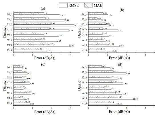
Figure 6.
Model performance on different time interval datasets: (a) 1-s interval; (b) 1-min interval; (c) 10-min interval; (d) 30-min interval.
It can be observed in Figure 6 that the LSTM network predicts the noise level with RMSE and MAE ranging between 1.77–3.20 dB(A) and 1.41–1.95 dB(A) in 1-s interval data sets respectively. Also, it forecasts the noise level to range between 0.71–1.64 dB(A) and 0.46–1.15 dB(A) in 1-min interval data sets for RMSE and MAE respectively while the noise level prediction by the LSTM network in 10-min interval data sets for RMSE and MAE ranges between 0.48–0.93 dB(A) and 0.31–0.69 dB(A) respectively. Lastly, the next level prediction made by the LSTM network in 30-min interval data sets for RMSE and MAE vary between 1.14–2.38 dB(A) and 0.73–1.57 dB(A) respectively.
Intuitively, the prediction results are fairly good based on the results of the above four groups of noise data in the LSTM model. For different monitoring points and different periods, the models behave differently. In general, the larger the time interval, the better the model performance, because the randomness of the noise is weakened as the time interval becomes larger. However, due to insufficient data volume, the number of records in the 30-min interval data set is limited, and the network is not trained enough to perform well.
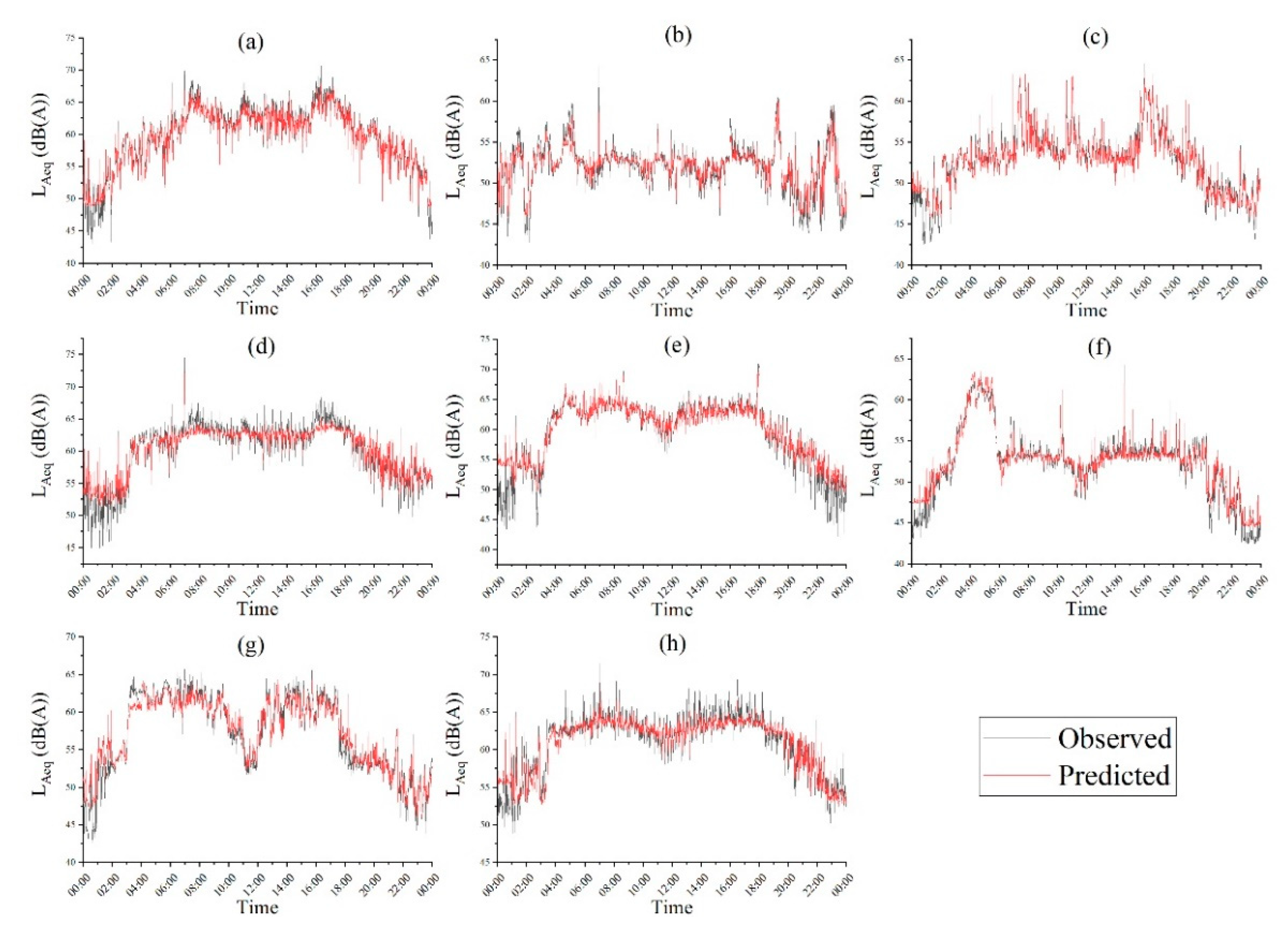
Considering the visualization of the data (too many drawing points may cause the image to appear messy), we used 10-min interval datasets throughout a monitoring day to compare the observation values and prediction values obtained by the LSTM model. As is displayed in Figure 7, the predicted values are fitted to the fluctuations of the actual values.
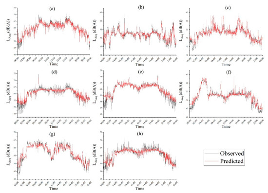
Figure 7.
Comparison of observed and predicted one-day noise value on different data sets: (a–h) dataset 01_a, 02_a, 03_a, 04_a, 01_b, 02_b, 03_b, 04_b.
3.5. Comparison of Prediction Accuracy
In this study, three classical prediction models were used to compare the prediction accuracy of the LSTM model. They are: random walk (RW) [57], stacked autoencoder (SAE) [18], and support vector machine (SVM) [58]. The RW model is the simplest, using the current state to predict the state of the next time, the formula is expressed as . SAE is a deep neural network model that has performed well in predicting time series in recent years. For SAE, we used a five-layer network, which includes three hidden layers. The optimizer is RMSprop, and the batch size is 256 for the optimal performance of the model. SVM is also one of the more typical algorithms in machine learning and has been widely used in classification and prediction problems. It solves the problem that the original data is linearly inseparable in the original space by selecting a kernel function to map the data to high-dimensional space. We chose the radial basis function (RBF) as the kernel function in this study, and set the penalty parameter C = 1000 and the kernel coefficient parameter gamma = 0.01. The autoregressive integrated moving average (ARIMA) model was also considered, but it was dismissed due to the long running time when processing large amounts of data.
Similarly, we used RMSE and MAE to evaluate the prediction accuracy of each model. For all models, the same data sets were used, and the model performance is shown in Figure 8.
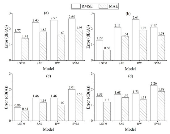
Figure 8.
Comparison of prediction results of different models at different time intervals: (a) 1-s interval; (b) 1-min interval; (c) 10-min interval; (d) 30-min interval.
It is vividly obvious from Figure 8 that, in the four prediction models for environmental noise time series, the performance of the LSTM network model proposed in this study is the best, and both the RMSE and MAE are the lowest.
4. Discussion
4.1. Superiority of the Proposed Noise Predicting Model
In this paper, the proposition of a model based on the LSTM neural network for predicting timely environmental noise was established. The model functions efficiently and saves time. The results demonstrated that the prediction ability of the model has high precision. At the same time, the proposed model outperforms the other three existing classic methods (SAE, RW, and SVM). The average running time of the model is several tens of seconds. From the results of Table 1 and Table 2, the setting and selection of parameters have little effect on the prediction results, so there is no need to be particularly cautious when selecting parameters. Moreover, a suitable set of parameters can be applied to all data sets of this study, and the parameters have certain universality. The predicted value can reflect the actual environmental noise level around the monitoring point and has a reference management role for environmental planners and government decision-makers.
4.2. Impact of Monitoring Point Location on Prediction Results
As shown in Figure 5, the four monitoring points are distributed in the same administrative district, but there are different features around different monitoring points. It is evident from Table 4 and Table 5 that the noise levels monitored by the four points are different. Among them, the 01 and 04 points are close to the road and construction site, the surrounding environment is generally noisy, and the average weekly noise is about 60 dB(A). The 02 point is relatively quiet because of the proximity to the water surface and residential areas. Its average weekly noise is about 50 dB(A). In overall, as illustrated in Figure 6, the model performs well on each dataset, but for the 1-s interval dataset, the prediction model has a larger error on the dataset of monitoring point 02. This is because the environment around point 02 is relatively quiet. When the model is making noise prediction, and it is actually predicting the typical value of this monitoring point noise, once there are other noise sources at point 02, the value predicted is much lower than the actual value, and the difference between the observed values and the predicted values is larger in contrast with other data sets, resulting in a larger error. On the other hand, when the time interval increases, this situation disappears, owing to the fact that some of the high noise values are averaged, and the model still predicts the typical value of this monitoring point. The error becomes infinitesimal when the model is fully trained.
4.3. Improvement of Prediction Method Based on Neural Network
This study focused on the prediction of noise in the short term. The noise levels of the monitoring points were predicted in seconds, minutes, 10 min, and 30 min, and contrasted with the measured values. The results revealed that there is a certain relationship between time interval and model performance. One possibility is that when the time interval increases, the randomness of the noise time series data set is weakened by the averaging operation, so the model can suitably fit the variation law of the noise level. Besides, previous studies have asserted that when the spatial and temporal diversity of noise sources is high, the prediction accuracy of the noise prediction model is reduced [59]. Poor performance was achieved by the model in 30-min interval data sets, probably because the LSTM network was not adequately trained and also few data sets were recorded. Wang et al. employed LSTM to forecast the reliability of the server system and found that the prediction accuracy of one month’s data set is higher than that of the 24-h data set, indicating that more training data has a positive impact on the prediction accuracy of the model [60]. Previous studies have developed many classic models of noise prediction, which attained good performance. However, with the development of Internet of Things technology and the promotion of big data, many classic models are no longer applicable in the case of large data volume. At this time, a new model capable of processing large data samples is needed to realize adequate management.
4.4. Recommendations for Environmental Noise Management
The predicted environmental noise has a particular reference for noise monitoring. The environmental noise standards for Chinese cities are divided into daytime (06:00–22:00) and nighttime (22:00–6:00). According to the Chinese environmental quality standard for noise [61], the study area belongs to residential, cultural, and educational institutions. The ambient noise limit is 55 dB(A) during the daytime and 45 dB during the nighttime. As shown in Table 4, during the two monitoring periods, except for monitoring point 02, the noise levels of monitoring points 01, 03, and 04 did not meet the standards. The prediction of noise in Figure 7 also reflects that the noise level of the monitoring point exceeds the standard. From this point of view, the prediction of environmental noise is conducive to a more comprehensive grasp of the noise level at the monitoring point, to promptly remind relevant departments to take practical actions.
There are many complaints about environmental noise in the city, if the predicted environmental noise can be regarded as a reference state to compare the actual observed noise level, it can facilitate the determination of a noise pollution incident that may be harmful to the health near the monitoring point, and further attract the attention of the environmental management department. On the other hand, the LSTM prediction model proposed in this study can predict the environmental noise at different time intervals, and can adapt to refined and diverse environmental management needs.
5. Conclusions
Conclusively, in the context of the rapid development of the environmental IoT, this study proposed a general method for predicting the timely environmental noise via the application of the LSTM network in a large data volume scenario and compared it with the performance of the classical model on the same data set, verifying the feasibility and effectiveness of the LSTM neural network in predicting environmental noise. However, due to the limitation of the duration of data collection time, this prediction has no way to verify the predictive ability of the LSTM network on the daily/monthly noise level. Nonetheless, as the time interval increases, the average noise level is more stable, and the randomness declines. Under the condition that the training samples are sufficient, the performance of the prediction model should be better. Furthermore, from this study, it is believed that the LSTM network can be applied simply to other noise data sets on predicting environmental noise, but different data sets may need to be re-adjusted. The shortcoming of this study is that the LSTM network structure used is relatively simple, and in the future, a more in-depth, broader and more powerful optimized LSTM model can be designed to improve accuracy. At the same time, the LSTM does not provide insight into the physical meaning of their parameters [62], in addition to time, more variables should be considered.
China’s past environmental noise monitoring method is mostly based on the statistical average. The monitoring data can only represent the overall average level of the specific time and place, which lacks understanding and application of environmental noise characteristics and acoustic laws, and in addition, lacks analysis of causes and effects. Establishing the connection between environmental noise and position, time, traffic, population, and other factors, replacing part of the monitoring work with prediction is the development direction of environmental noise evaluation. The monitoring and evaluation methods should be optimized from this perspective to make the monitoring results more in-depth and representative.
Author Contributions
R.D., X.Z., and M.Z. conceived the general idea of the paper. X.Z. and M.Z. designed the methodology and the model. All authors analyzed and discussed the results. R.D. and X.Z. wrote this paper. All authors have read and agreed to the published version of the manuscript.
Funding
This study was funded by The National Key Research and Development Program of China (No. 2016YFC0503605).
Conflicts of Interest
The authors declare no conflict of interest.
References
- Al-Fuqaha, A.; Guizani, M.; Mohammadi, M.; Aledhari, M.; Ayyash, M. Internet of things: A survey on enabling technologies, protocols, and applications. IEEE Commun. Surv. Tutor. 2015, 17, 2347–2376. [Google Scholar] [CrossRef]
- Zanella, A.; Bui, N.; Castellani, A.; Vangelista, L.; Zorzi, M. Internet of things for smart cities. IEEE Internet Things J. 2014, 1, 22–32. [Google Scholar] [CrossRef]
- Chen, S.; Xu, H.; Liu, D.; Hu, B.; Wang, H. A vision of IoT: Applications, challenges, and opportunities with China perspective. IEEE Internet Things J. 2014, 1, 349–359. [Google Scholar] [CrossRef]
- Schaffers, H.; Komninos, N.; Pallot, M.; Trousse, B.; Nilsson, M.; Oliveira, A. Smart cities and the future internet: Towards cooperation frameworks for open innovation. In Proceedings of the Future Internet Assembly, Budapest, Hungary, 17–19 May 2011; pp. 431–446. [Google Scholar]
- Maisonneuve, N.; Stevens, M.; Niessen, M.E.; Hanappe, P.; Steels, L. Citizen noise pollution monitoring. In Proceedings of the 10th Annual International Conference on Digital Government Research: Social Networks: Making Connections between Citizens, Data and Government, Puebla, Mexico, 17–20 May 2009; pp. 96–103. [Google Scholar]
- Camero, A.; Alba, E. Smart City and information technology: A review. Cities 2019, 93, 84–94. [Google Scholar] [CrossRef]
- Dzhambov, A.M.; Dimitrova, D.D. Urban green spaces effectiveness as a psychological buffer for the negative health impact of noise pollution: A systematic review. Noise Health 2014, 16, 157–165. [Google Scholar] [CrossRef]
- Clark, C.; Crumpler, C. Evidence for Environmental Noise Effects on Health for the United Kingdom Policy Context: A Systematic Review of the Effects of Environmental Noise on Mental Health, Wellbeing, Quality of Life, Cancer, Dementia, Birth, Reproductive Outcomes, and Cognition. Int. J. Environ. Res. Public Health 2020, 17, 393. [Google Scholar] [CrossRef]
- Law of the People’s Republic of China on Environmental Noise Pollution Prevention; The Standing Committee of the National People’s Congress: Beijing, China, 1996.
- López-Pacheco, M.G.; Sánchez-Fernández, L.P.; Molina-Lozano, H. A method for environmental acoustic analysis improvement based on individual evaluation of common sources in urban areas. Sci. Total Environ. 2014, 468, 724–737. [Google Scholar] [CrossRef]
- China Environmental Noise Pollution Prevention Report. 2018. Available online: http://dqhj.mee.gov.cn/dqmyyzshjgl/zshjgl/201808/t20180803_447713.shtml (accessed on 3 August 2018).
- Trial Big Data of Beijing-Tianjin-Hebei Environmental Resources Released: Noise Pollution Cases Accounted for 73% of The Total Number of Cases. Available online: http://china.cnr.cn/ygxw/20180604/t20180604_524257319.shtml (accessed on 4 June 2018).
- Aurbach, L.J. Aviation Noise Abatement Policy: The Limits on Federal Intervention. Urb. Law. 1977, 9, 559. [Google Scholar]
- Gesetz Zum Schutz Gegen Fluglärm. In Bundesgesetzblatt; Teil I; Bundesanzeiger Verlag GmbH: Köln, Germany, 1971; pp. 282–287.
- Filippone, A. Aircraft noise prediction. Prog. Aerosp. Sci. 2014, 68, 27–63. [Google Scholar] [CrossRef]
- Ollerhead, J. The CAA Aircraft Noise Contour Model: ANCON Version 1; Civil Aviation Authority: Cheltenham, UK, 1992. [Google Scholar]
- Pietrzko, S.; Bütikofer, R. FLULA-Swiss aircraft noise prediction program. In Proceedings of the Innovation in Acoustics and Vibration, Annual Conference of the Australian Acoustical Society, Adelaide, Australia, 13–15 November 2002; pp. 13–15. [Google Scholar]
- Ausejo, M.; Recuero, M.; Asensio, C.; Pavon, I.; Lopez, J.M. Study of Precision, Deviations and Uncertainty in the Design of the Strategic Noise Map of the Macrocenter of the City of Buenos Aires, Argentina. Environ. Modeling Assess. 2010, 15, 125–135. [Google Scholar] [CrossRef]
- Tsai, K.T.; Lin, M.D.; Chen, Y.H. Noise mapping in urban environments: A Taiwan study. Appl. Acoust. 2009, 70, 964–972. [Google Scholar] [CrossRef]
- Wang, H.B.; Cai, M.; Yao, Y.F. A modified 3D algorithm for road traffic noise attenuation calculations in large urban areas. J. Environ. Manag. 2017, 196, 614–626. [Google Scholar] [CrossRef]
- Zambon, G.; Roman, H.; Smiraglia, M.; Benocci, R. Monitoring and prediction of traffic noise in large urban areas. Appl. Sci. 2018, 8, 251. [Google Scholar] [CrossRef]
- Kumar, K.; Jain, V.K. Autoregressive integrated moving averages (ARIMA) modelling of a traffic noise time series. Appl. Acoust. 1999, 58, 283–294. [Google Scholar] [CrossRef]
- Garg, N.; Soni, K.; Saxena, T.K.; Maji, S. Applications of AutoRegressive Integrated Moving Average (ARIMA) approach in time-series prediction of traffic noise pollution. Noise Control Eng. J. 2015, 63, 182–194. [Google Scholar] [CrossRef]
- Gajardo, C.P.; Morillas, J.M.B.; Gozalo, G.R.; Vilchez-Gomez, R. Can weekly noise levels of urban road traffic, as predominant noise source, estimate annual ones? J. Acoust. Soc. Am. 2016, 140, 3702–3709. [Google Scholar] [CrossRef]
- Golmohammadi, R.; Abolhasannejad, V.; Soltanian, A.R.; Aliabadi, M.; Khotanlou, H. Noise Prediction in Industrial Workrooms Using Regression Modeling Methods Based on the Dominant Frequency Cutoff Point. Acoust. Aust. 2018, 46, 269–280. [Google Scholar] [CrossRef]
- Rahmani, S.; Mousavi, S.M.; Kamali, M.J. Modeling of road-traffic noise with the use of genetic algorithm. Appl. Soft Comput. 2011, 11, 1008–1013. [Google Scholar] [CrossRef]
- Wang, C.; Chen, G.; Dong, R.; Wang, H. Traffic noise monitoring and simulation research in Xiamen City based on the Environmental Internet of Things. Int. J. Sustain. Dev. World Ecol. 2013, 20, 248–253. [Google Scholar] [CrossRef]
- Iannace, G.; Ciaburro, G.; Trematerra, A. Wind Turbine Noise Prediction Using Random Forest Regression. Machines 2019, 7, 69. [Google Scholar] [CrossRef]
- Torija, A.J.; Ruiz, D.P. A general procedure to generate models for urban environmental noise pollution using feature selection and machine learning methods. Sci. Total Environ. 2015, 505, 680–693. [Google Scholar] [CrossRef]
- Van Den Berg, F.; Eisses, A.R.; Van Beek, P.J. A model based monitoring system for aircraft noise. J. Acoust. Soc. Am. 2008, 123, 3151. [Google Scholar] [CrossRef]
- Quintero, G.; Balastegui, A.; Romeo, J. Annual traffic noise levels estimation based on temporal stratification. J. Environ. Manag. 2018, 206, 1–9. [Google Scholar] [CrossRef]
- Brambilla, G.; Lo Castro, F.; Cerniglia, A.; Verardi, P. Accuracy of temporal samplings of environmental noise to estimate the long-term Lden value. In Proceedings of the INTER-NOISE and NOISE-CON Congress and Conference Proceedings, Istanbul, Turkey, 28–31 August 2007; pp. 4082–4089. [Google Scholar]
- D’Hondt, E.; Stevens, M.; Jacobs, A. Participatory noise mapping works! An evaluation of participatory sensing as an alternative to standard techniques for environmental monitoring. Pervasive Mob. Comput. 2013, 9, 681–694. [Google Scholar] [CrossRef]
- Shu, H.Y.; Song, Y.; Zhou, H. RNN Based Noise Annoyance Measurement for Urban Noise Evaluation. In Proceedings of the IEEE Region 10 Conference (TENCON), Penang, Malaysia, 5–8 November 2017; pp. 2353–2356. [Google Scholar]
- Iannace, G.; Ciaburro, G.; Trematerra, A. Heating, Ventilation, and Air Conditioning (HVAC) Noise Detection in Open-Plan Offices Using Recursive Partitioning. Buildings 2018, 8, 169. [Google Scholar] [CrossRef]
- Iannace, G.; Ciaburro, G.; Trematerra, A. Fault Diagnosis for UAV Blades Using Artificial Neural Network. Robotics 2019, 8, 59. [Google Scholar] [CrossRef]
- Deng, L.; Yu, D. Deep learning: Methods and applications. Found. Trends Signal Process. 2014, 7, 197–387. [Google Scholar] [CrossRef]
- Lv, Y.; Duan, Y.; Kang, W.; Li, Z.; Wang, F.-Y. Traffic flow prediction with big data: A deep learning approach. IEEE Trans. Intell. Transp. Syst. 2015, 16, 865–873. [Google Scholar] [CrossRef]
- Goodfellow, I.; Bengio, Y.; Courville, A.; Bengio, Y. Deep Learning; MIT Press: Cambridge, UK, 2016; Volume 1. [Google Scholar]
- Nelson, D.M.; Pereira, A.C.; de Oliveira, R.A. Stock market’s price movement prediction with LSTM neural networks. In Proceedings of the 2017 International Joint Conference on Neural Networks (IJCNN), Anchorage, AK, USA, 14–19 May 2017; pp. 1419–1426. [Google Scholar]
- Zhang, Q.; Wang, H.; Dong, J.; Zhong, G.; Sun, X. Prediction of sea surface temperature using long short-term memory. IEEE Geosci. Remote Sens. Lett. 2017, 14, 1745–1749. [Google Scholar] [CrossRef]
- Graves, A.; Jaitly, N.; Mohamed, A.-R. Hybrid speech recognition with deep bidirectional LSTM. In Proceedings of the 2013 IEEE Workshop on Automatic Speech Recognition and Understanding (ASRU), Olomouc, Czech Republic, 8–12 December 2013; pp. 273–278. [Google Scholar]
- Chowdhury, S.A.; Zamparelli, R. RNN simulations of grammaticality judgments on long-distance dependencies. In Proceedings of the 27th International Conference on Computational Linguistics, Santa Fe, NM, USA, 20–26 August 2018; pp. 133–144. [Google Scholar]
- Hochreiter, S.; Schmidhuber, J. Long short-term memory. Neural Comput. 1997, 9, 1735–1780. [Google Scholar] [CrossRef]
- Gers, F.A.; Schmidhuber, J.; Cummins, F. Learning to forget: Continual prediction with LSTM. Neural Comput. 2014, 12, 2451–2471. [Google Scholar] [CrossRef]
- Graves, A.; Schmidhuber, J. Framewise phoneme classification with bidirectional LSTM and other neural network architectures. Neural Netw. 2005, 18, 602–610. [Google Scholar] [CrossRef]
- Colah. Understanding LSTM Networks. Available online: http://colah.github.io/posts/2015-08-Understanding-LSTMs/ (accessed on 27 August 2015).
- Sundermeyer, M.; Schlüter, R.; Ney, H. LSTM neural networks for language modeling. In Proceedings of the Thirteenth Annual Conference of the International Speech Communication Association, Portland, OR, USA, 9–13 September 2012. [Google Scholar]
- Mahdavinejad, M.S.; Rezvan, M.; Barekatain, M.; Adibi, P.; Barnaghi, P.; Sheth, A.P. Machine learning for Internet of Things data analysis: A survey. Digit. Commun. Netw. 2018, 4, 161–175. [Google Scholar] [CrossRef]
- Tian, Y.; Pan, L. Predicting short-term traffic flow by long short-term memory recurrent neural network. In Proceedings of the 2015 IEEE international conference on smart city/SocialCom/SustainCom (SmartCity), Chengdu, China, 19–21 December 2015; pp. 153–158. [Google Scholar]
- Greff, K.; Srivastava, R.K.; Koutnik, J.; Steunebrink, B.R.; Schmidhuber, J. LSTM: A Search Space Odyssey. IEEE Trans. Neural Netw. Learn. Syst. 2017, 28, 2222–2232. [Google Scholar] [CrossRef]
- Ruder, S. An overview of gradient descent optimization algorithms. arXiv 2016, arXiv:1609.04747. [Google Scholar]
- Kingma, D.P.; Ba, J. Adam: A method for stochastic optimization. arXiv 2014, arXiv:1412.6980. [Google Scholar]
- Quan, Y.; Wang, C.P.; Wang, H.W.; Su, X.D.; Dong, R.C. Design and Application of Noise Monitoring System Based on Wireless Sensor Network. Environ. Sci. Technol. 2012, 35, 255–258. [Google Scholar]
- Brooks, C. Introductory Econometrics for Finance; Cambridge University Press: Cambridge, UK, 2019. [Google Scholar]
- Bouktif, S.; Fiaz, A.; Ouni, A.; Serhani, M. Optimal deep learning lstm model for electric load forecasting using feature selection and genetic algorithm: Comparison with machine learning approaches. Energies 2018, 11, 1636. [Google Scholar] [CrossRef]
- Spitzer, F. Principles of Random Walk; Springer Science & Business Media: Berlin/Heidelberg, Germany, 2013; Volume 34. [Google Scholar]
- Sapankevych, N.I.; Sankar, R. Time series prediction using support vector machines: A survey. IEEE Comput. Intell. Mag. 2009, 4, 24–38. [Google Scholar] [CrossRef]
- Oiamo, T.H.; Davies, H.; Rainham, D.; Rinner, C.; Drew, K.; Sabaliauskas, K.; Macfarlane, R. A combined emission and receptor-based approach to modelling environmental noise in urban environments. Environ. Pollut. 2018, 242, 1387–1394. [Google Scholar] [CrossRef]
- Wang, H.B.; Yang, Z.P.; Yu, Q.; Hong, T.J.; Lin, X. Online reliability time series prediction via convolutional neural network and long short term memory for service-oriented systems. Knowl. Based Syst. 2018, 159, 132–147. [Google Scholar] [CrossRef]
- Ministry of Environmental Protection. Environmental Standard for Noise; In Chinese; Ministry of Environmental Protection: Beijing, China, 2008.
- Tomić, J.; Bogojević, N.; Pljakić, M.; Šumarac-Pavlović, D. Assessment of traffic noise levels in urban areas using different soft computing techniques. J. Acoust. Soc. Am. 2016, 140, EL340–EL345. [Google Scholar] [CrossRef] [PubMed]
© 2020 by the authors. Licensee MDPI, Basel, Switzerland. This article is an open access article distributed under the terms and conditions of the Creative Commons Attribution (CC BY) license (http://creativecommons.org/licenses/by/4.0/).

