Article

Artificial Neural Network for Vertical Displacement Prediction of a Bridge from Strains (Part 2): Optimization of Strain-Measurement Points by a Genetic Algorithm under Dynamic Loading

1
Department of Civil and Environmental Engineering, Yonsei University, College of Engineering, 50, Yonsei-ro, Seodaemun-gu, Seoul 03722, Korea
2
Department of Civil Engineering, The University of Tokyo, 7-3-1 Hongo, Bunkyo-ku, Tokyo 790-8577, Japan
*
Author to whom correspondence should be addressed.
Appl. Sci. 2020, 10(3), 777; https://doi.org/10.3390/app10030777
Submission received: 22 November 2019 / Revised: 11 January 2020 / Accepted: 16 January 2020 / Published: 22 January 2020

Abstract

:
Bridge displacements are one of the most important physical values in evaluating the health of bridges. However, the direct measurement of bridge displacements is not easy due to various factors, such as installation location and cost. For that reason, in a previous study (part 1), a method for predicting bridge displacements from strains was proposed using an artificial neural network (ANN), which has a strong ability in data mapping. In this paper, to predict the overall displacements from a small number of strains more efficiently, a method to optimize the number and locations of strain-measurement points was proposed using the genetic algorithm (GA), which is widely used for global optimization. To verify the proposed methods, two cases, a simple beam under sinusoidal loads and a girder bridge under vehicle loads, are carried out through numerical analysis. Also, a laboratory experiment is carried out with a vibrating cantilever beam. The results indicate that the predicted displacements from at least two strains at the optimized locations show good agreements with displacements by numerical analysis and measurements. The results suggest that the proposed method (optimization of strain-measurement points) is very efficient and can be applied in the actual field.

1. Introduction

After an infrastructure is opened to the public, it gradually deteriorates because of unexpected loading, temperature fluctuations, and/or numerous other environmental factors. To ensure the durability and integrity of infrastructure from these factors, it is important to monitor global structural behavior. In particular, bridges are one of the most important infrastructures. Hence, bridge behavior can provide considerable information. The intuitive global behavior of bridges not only predicts the loads applied to them, such as that in weigh-in-motion systems [1], but also evaluates the structural condition. Also, the long-term variation in the displacements provides a rationale for evaluating the degradation and aging of a structure. Although the displacements provide important information regarding intuitive global behavior, it is difficult to measure them directly. For example, to directly measure the relative displacement of a structure using instruments (such as mechanical dial gauges, linear potentiometers, and linear variable differential transducers) fixed bases are required. However, it is difficult to find fixed bases because most bridges are constructed high from the ground or cross the seas and rivers [2]. The measurement cost with the use of a supporting systems for fixed bases is sometimes very expensive.
To overcome the difficulty of direct measurement of bridge displacements, various studies have been conducted to measure bridge displacements through various direct measurement approaches. Xu et al. [3] researched the measurement of bridge displacement using a global positioning system (GPS). GPS shows high accuracy but has the disadvantage of being expensive. It is also affected by weather because it needs to communicate with satellites. Nassif et al. [4] and Pieraccini et al. [5] researched the measurement of bridge displacement using a laser doppler vibrometer (LDV) and Lee et al. [2], Stephen et al. [6], Olaszek [7], and Wahbeh et al. [8] researched using optic devices.
Studies on the prediction of displacement from relatively easily measurable data, such as acceleration and strain, have also been researched. Faulkner [9] and Park et al. [10] proposed a method for predicting bridge displacement from measured acceleration. Theoretically, displacements can be calculated by double integration of acceleration. However, because it is difficult to determine the initial condition (displacement, velocity) for integration in advance, it seems to be unreliable. Wang et al. [11], Chung et al. [12], Glaser et al. [13], Kang et al. [14], Rapp et al. [15], Kim et al. [16], and Kim and Cho [17] proposed a method for predicting displacement from strain. The curvature or modal shape of the structure can be obtained from the measured strains. Finally, the displacements can be predicted from the curvature or modal shape. Theoretically, the proposed method is feasible. However, the actual bridges in service are complex, and the load is irregular. Therefore, it is not easy to theoretically predict displacement.
Moon et al. [18] suggested a method for predicting the overall bridge displacements from strains using an artificial neural network (ANN). The relationship between strains and displacements is difficult to justify theoretically in the case of complex structures. However, if an ANN is utilized, the relation between strains and the displacements can be justified better than beam theory because an ANN justifies the relation based on data training rather than theory. In the previous paper [18], the feasibility of displacement prediction from strain was confirmed by numerical model.
In this paper, as an extension of previous research, a method for optimizing the number and locations of strain-measurement points using a genetic algorithm (GA) is proposed to efficiently and accurately predict the displacements with fewer strains. Since the ANN trains the relationship between strain (= input) and displacement (= output), the number and locations of strain-measurement points used as input have a significant effect on the training results. In general, the larger the number of strains used as input, the higher the accuracy of displacement prediction. Also, advances in sensor technology make it possible to install large numbers of sensors in structures [19,20]. However, this can cause some economic problems such as cost of installations, data acquisition and analysis, etc. [20,21]. In addition, even when the same number of strains is used, the displacement prediction accuracy varies greatly depending on the location of the strains. In the field, the number and locations of sensor installations may be determined by one’s intuition or empirical knowledge [22]. However, this reduces the usefulness of the measured data, resulting in economic and time loss. Since the number and locations of sensors have a large impact on data utilization, considerable research has been conducted for sensor optimization [22,23,24,25,26,27,28,29,30,31,32,33,34,35,36,37,38]. In those researches, many intelligent algorithms such as GAs, particle swarm, glowworm swarm, artificial bee colony, monkey, ant colony, etc., have been utilized for the optimization. As mentioned, various algorithms have been used for optimization, but methods to optimize the number and locations of strains required for ANNs to predict displacements have not been studied. Hence, in this study, the number and locations of strain-measurement points are optimized using a genetic algorithm. The locations of strain-measurement points as optimization variables and mean squared error of the trained ANN as the objective function are used for the optimization. To verify the proposed method, two cases, a simple beam and bridge under dynamic loading, were carried out by utilizing the numerical models. Also, a laboratory experiment was carried out with the steel cantilever beam. Using the commercial program ABAQUS, the two numerical models are made and analyzed for obtaining ANN training and test data. The neural network toolbox in MATLAB is utilized for ANN training and tests. Also, the global optimization toolbox in MATLAB is used for optimizing the number and locations of strain-measurement points based on a GA.

2. Methods

In this section, a brief background on artificial intelligence is presented to understand ANNs and GAs. Additionally, the method to optimize the number and locations of strain-measurement points using both an ANN and a GA is described.

2.1. Artificial Neural Networks (ANNs)

An ANN is a computer model inspired by the neural networks observed in biology. McCulloch and Pitts pioneered the study on ANNs [39]. ANNs were originally developed as an algorithm to describe the capabilities of biological neural systems [40]. Thereafter, various types of ANNs have been developed such as the most widely used multilayer feed-forward ANN [41]. This type of ANN comprises an input layer, one or more hidden layers, and an output layer (see Figure 1).
The advantage of an ANN is that it can be used to map the correlation between the input and output data in a complex nonlinear or ambiguous relationship. To accurately determine the relationship between the inputs and the outputs, the ANN should be trained. The most commonly used algorithm for training is backpropagation [42]. Through this algorithm, the trained ANN can accurately predict data similar to, but not the same as, the learning data [43]. The most commonly used error function for training is mean squared error(MSE).
M S E = 1 N i = 1 N ( T i P i ) 2
In Equation (1), T is the target value, P is the predicted value, and N is the number of data. The closer the MSE is to zero, the higher the prediction accuracy.
ANNs have been used successfully in civil engineering applications. Yan et al. [44] predicted the concrete bond strength of a glass fiber-reinforced polymer bar using an ANN optimized via a GA. Najjar and Basheer [45] predicted soil characteristics and uncertainty using an ANN. Shahin et al. [46] used an ANN to predict the settlement of shallow foundations. Jan et al. [47] predicted the displacement of an excavation using an ANN. Although ANNs have been used in various fields in civil engineering, they have rarely been applied to predict the displacement of a bridge.

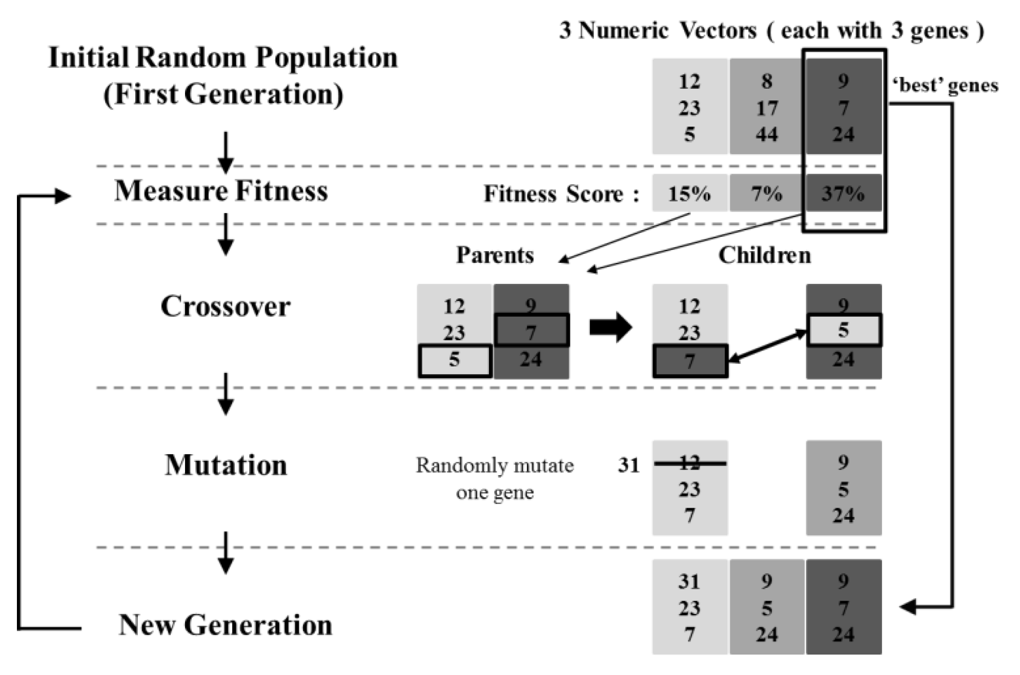
2.2. Genetic Algorithm (GA)

A GA is an optimization algorithm developed by Holland [48]. A GA imitates the process of evolution of biological species by natural selection [41]. In other words, analogous to the evolution of creatures, the strong species (with a high fitness score) evolve into the next generation, whereas the weak species (with a low fitness score) disappear from that generation. Figure 2 shows the GA concept. In a GA, the new possible solutions are iterated via crossover and mutation. The crossover is the main operator that helps in randomly selecting two-parent numeric vectors and swapping their segments [49]. The other is a mutation wherein an operator is used to change the gene of an existing numeric vector to an arbitrary gene. The GA repeats this process until the optimal numeric vector (i.e., with the highest fitness score) to a problem is found. The advantage of GAs is that they can be applied to complex optimization problems [50]. In addition, the probability of being trapped at a local minimum is less than that in a typical optimization technique. Because of these advantages, GAs have been widely used in many optimization problems. Faghihi et al. [51] optimized a construction scheduling problem using GAs. Chandwani et al. [52] employed a GA to predict the slump of concrete based on the optimized weight and bias of an ANN. RazaviAlavi and AbouRizk [53] optimized site layout and construction plan variables. Moreover, a method for planning an efficient construction project was proposed using GAs.

2.3. Optimizing the Number and Locations of Strain-Measurement Points

Figure 3 shows a flowchart of the process wherein the GA and ANN are used for optimizing the number and locations of strain-measurement points. First, the number (ns) of strain-measurement points is selected. Then, the GA optimizes the location of ns strain-measurement points as optimization variables. The MSE of the trained ANN is used as an objective function. Using the ns strains at the locations generated by the GA as inputs and the overall displacements as outputs, the ANN is trained. Then, the GA evaluates the fitness values for all populations for each generation. Using the selection, the crossover, and mutations, the GA continues to evaluate the fitness values. We used stochastic uniform function for the selection, which helps various parents to be selected for the next generation. We used scattered function for the crossover and Gaussian function for the mutation. The GA continues to iterate to determine the minimum MSE until the stopping criterion is satisfied. For the ANN architecture, one hidden layer is used in consideration of the computational time. Additionally, the number of nodes in the hidden layer is selected the same as the number of input values, as suggested by [55]. The parameters used in the training of the ANN are shown in Table 1.

3. Verification through a Simple Beam Under Sinusoidal Loads

3.1. Collecting Training and Test Data

To verify the proposed method, a simple beam with a span of 3000 mm (see Figure 4) was utilized. Because simple beams are used as the main girder in bridges, it is very important to predict the displacements of simple beams. To collect the training and test data, a sine load of 1 kN with periods of 1, 0.5, and 0.1 s was applied to the center of the beam for 1 s. For example, in the case of the 0.5 s period, a total of two cycles was applied. To obtain the data, numerical analysis was carried out. Additionally, the beam was divided into 41 nodes (interval 75 mm) to obtain the strains and displacements at each time step. Therefore, one dataset consisted of 41 strains (input) and 41 displacements (output). Figure 5 shows the graph for sine loads. Also, Table 2 shows the number of datasets.

3.2. Optimization Results

As proposed in Section 2.2., the location of ns strain-measurement points was optimized in the order of four, three, and two. The GA optimized the location of the strain-measurement points as optimization variables. The MSE of the trained ANN was used as an objective function. The ANN architecture of ns-ns-41 (no. of inputs–no. of hidden nodes–no. of outputs) was selected. The population size was 40, and generations were iterated until the minimum fitness value was not updated over more than 50 iterations. Table 3 shows the optimization results. Means squared error (MSE), and regression value (R) were used as the results of ANN training and testing. MSE is a function that shows the ANN training accuracy in general. The closer to 0, the higher the accuracy. Since MSE may be influenced by the absolute values of the predicted values, the regression (R) value was additionally used to evaluate the training accuracy. The R-value represents the degree of correlation between the target and the prediction. An R-value tending to 1 represents a high correlation. Figure 6 shows the optimized locations for each number of strain-measurement points on the beam.
When four strains at the optimized locations (450, 1500, 2250, and 2700 mm) were used as the ANN input, the MSE and R of the trained ANN were 0.0113 and 0.9999, respectively. For comparison, the MSE and R-values are presented in Table 3 when four strains at arbitrary locations (75, 150, 2775, and 2850 mm) were used as the ANN input. The MSE and R of the trained ANN were 8.0591 and 0.9945, respectively. Even if the same number of strains were used, it can be seen that the prediction accuracy would differ significantly depending on the location. Likewise, a similar tendency was shown when three and two strains were used. In the case of the strains at the optimized locations, the MSE was 0.0113, 0.0073, and 0.0513 for four, three, and two strains, respectively. The R-value was 0.9999 in all cases. The MSE close to 0 and the R close to 1 showed that the overall displacement prediction accuracy was very high even when using two strains at the optimized locations. Although the ANN was well-trained, the prediction accuracy of the data that was not used in the training was significantly lower than the training accuracy. This situation is called overfitting. To test for overfitting and prediction accuracy, strains from the test dataset (periods 0.8 s) were input into the trained ANN, and the displacements predicted using the trained ANN were then compared with those predicted by the numerical analysis. When the displacements were predicted from four, three, and two strains, the MSEs were 0.0125, 0.0072, and 0.0524, respectively. Since there was no significant difference from the training MSE, overfitting did not occur, and the predictive accuracy of the trained ANN was very high. In Figure 7 and Figure 8, the graphs are plotted for an intuitive comparison. Figure 7 shows the displacements over time at the beam center, depending on the number of strains. It can be seen that the fluctuation was very large when the strains at the arbitrary locations were used. However, when the strains at the optimized locations were used, the predicted displacements showed good agreements with the numerical results regardless of the number of strains. Figure 8 shows the beam displacement shape at t = 1 s, where the largest displacement occurs. In the case of using strains at arbitrary locations, the overall displacement shape was similar, but it can be seen that there was a large difference from the numerical results. However, when the strains at the optimized locations were used, the displacement shape was very similar to the numerical results. From the results, it could be seen that the ANN can predict the displacement shape of the beam under the dynamic load with very high accuracy when using the strain at the optimized locations by GA.
Difference = DisplacementFEM − DisplacementANN

4. Application to a Plate Girder Bridge under Vehicle Load

4.1. Collecting Training and Test Data

In Section 3.1., the proposed optimization method was verified using a simple beam. In this section, an I-shaped steel plate 5-girder bridge was utilized for verification of the proposed optimization method. Moon et al. [18] confirmed the predictability of displacements from the strains of a bridge under vehicle load in a previous paper. Eleven displacements were predicted from eleven strains per girder. In this paper, the number and locations of strain-measurement points needed to predict eleven displacements for the same bridge model were optimized by GA. The specifications of the bridge model are shown in Table 4.
Three types of vehicles—passenger cars, buses, and trucks—were considered for vehicle load. Additionally, it was assumed that they moved at constant speeds (40 km/h, 60 km/h, and 80 km/h) across the bridge. The numerical models of cars, buses, and trucks were made by vehicles proposed by Zuo and Nayfeh [56], Ahmed et al. [57], and Li [58]. The numerical model was verified by comparison with experimental values [59,60]. Figure 9 shows the numerical bridge model and section of girder.
Utilizing a Pearson type III traffic distribution theory [61], a total of 25 load scenarios were created for each vehicle speed. Using the 25 load scenario for each speed, numerical analysis was carried out. From the analysis, eleven strains and displacement measurement points were selected at uniform intervals of 3.6 m below the flange of each girder (Figure 10) to obtain ANN training and test data. Therefore, a total of 55 strains (11 points × 5 girders, input) and displacements (11 points × 5 girders, output) were collected. The time step (Δt) was 0.01 s, and the vehicles were loaded for a total of 8 s. Table 5 shows the organization of training and test datasets obtained from the analysis. Also, the detail description for the numerical analysis and numerical model can be found in part 1 of the paper [18].

4.2. Optimization Results

According to the proposed method in Section 2.2., the locations of ns strain-measurement points per girder as optimization variables were optimized in the order of four, three, and two. Since the bridge model has five girders, the total number of strain-measurement points was 5 × ns. Additionally, it was assumed that the location of ns strain-measurement points were all the same for five girders. Fifty populations per generation were evaluated based on the objective function (= MSE). Additionally, the optimization was set to end when the minimum fitness value had not changed in more than 50 iterations. In Figure 11, the change in fitness value according to generation is shown.
In Figure 11, the MSE gradually decreases with the generations even though there are differences depending on the number of strain measurements. Table 6 and Figure 12 show the optimized locations of strain-measurement points and the training MSE and R for the optimized locations. The training results for arbitrary locations are also presented in Table 6. Using eleven strains and using two strains, the MSE (×10−3) was 1.2007 and 2.5370, respectively. Although the number of strain-measurement points decreased by more than five times, there was no significant difference in MSE values. When comparing the R-values using eleven strains and two strains, the R-values were 0.9988 and 0.9975, respectively. It is also considered that there was no significant difference in the R-value. In the case of four strains for arbitrary and optimized locations, the training MSE (×10−3) was 5.4946 and 1.4268, respectively. In other words, when the strains at the optimized locations were used as the ANN input, the training accuracy was much higher. The same result occurred even when three and two strains were used. In the case of the optimized locations, the number of strains was four, three, and two, and the training MSE (×10−3) tended to increase slightly to1.4268, 1.7511, and 2.5370, respectively. However, since the values were all very close to zero, even when two strains at the optimized locations were used as ANN input, very high training accuracy can be expected. In addition, the R-value was close to 1 for all optimized positions. From the training results, the effectiveness of the GA for the location optimization of strains required for displacement prediction could be confirmed. To test for overfitting and prediction accuracy of the trained ANN, three test datasets (40 km/h, 60 km/h, and 80 km/h) that were not used for training were utilized. Table 7 shows the test results for the test dataset. When the strains at the optimized locations obtained from numerical analysis were input into the trained ANN, the trained ANN predicted displacements from the strains. In the case of using four strains at arbitrary locations, the MSE (×10−3) was 1.7815, 1.7924, and 7.6117 for 40 km/h, 60 km/h, and 80 km/h, respectively. Additionally, using four strains at the optimized locations, the MSE (×10−3) was 0.7987, 0.4805, and 4.7009 for 40 km/h, 60 km/h, and 80 km/h, respectively. Comparing the two cases, it could be seen that the displacement prediction accuracy was very high when the strains at the optimized locations were used. Similar results were obtained for three and two strains. Using strains at the optimized locations, the MSE (×10−3) for four, three, and two strains was 0.7987, 0.8830, and 1.1249, respectively, for 40 km/h. The MSE increased slightly as the number of strains decreased but was still close to zero. From the results, as with the training accuracy, it could be confirmed that the prediction accuracy of the test data was very high. For an intuitive comparison, the predicted displacements are presented in Figure 13, Figure 14, Figure 15, Figure 16, Figure 17 and Figure 18. Figure 13 shows the change in displacements over time at the midpoint of the center girder (CG) for strains at arbitrary and optimized locations for 40 km/h, which is expected to produce the maximum displacements. In addition, the differences between the numerical analysis results and predicted displacements are plotted. In both arbitrary and optimized locations, as the number of strains decreased, the difference from the numerical analysis results increased. In particular, in the case of arbitrary locations, the difference according to the number of strains was large, and it could be seen that there was an overall fluctuation. In the case of the optimized locations, the difference in the number of strains was not large and predicted displacements showed good agreements with the overall numerical analysis. Figure 14 shows the overall displacement shape of the center girder (CG) at t = 6.52 s, at which time the maximum displacement occurred. As in Figure 14, for arbitrary locations, the difference between predicted displacements and numerical results was very large. For the optimized locations, predicted displacements showed good agreements with numerical analysis regardless of the number of strains. The same results are shown for the test datasets of 60 km/h and 80 km/h (Figure 15, Figure 16, Figure 17 and Figure 18). From the results, as in the simple beam, the effectiveness of the GA was confirmed in optimizing the locations of the strain-measurement points required for displacement prediction of a bridge under vehicle load.

5. Experimental Verification with Cantilever Beam

In order to predict the displacements of a vibrating cantilever beam using the proposed method, a laboratory test was performed (Figure 19). The cross-section of the beam was a 50 × 5 mm rectangle. The elastic modulus of the steel cantilever beam was 200 GPa and the unit weight was 7850 kgf/m3. In order to vibrate the beam, initial displacements at the end of the beam were introduced. Training data were obtained from the numerical model and test data were obtained from actual measurements. First, strains and displacements data for the training were obtained from numerical model. The two initial displacement conditions of 1 cm and 3 cm were introduced. A total 4002 training datasets were obtained from the numerical analysis for 10 s with 200 Hz sampling frequency. One dataset consisted of 52 strains and 52 displacements with 1020 mm beams spaced at 20 mm intervals.
Using those training data and the proposed method (GA and ANN), the locations of strain-measurement points were optimized for two numbers. Then, the optimized locations were 100 mm and 700 mm. To obtain test data, strain sensors were installed in three locations (100, 600, and 700 mm), including the optimized locations. Also, laser displacement sensors were installed at three points (400, 700, and 1000 mm) to compare the accuracy of the predicted displacements (Table 8). The initial displacement of 2 cm was introduced on the beam. During vibration, strains and displacement were measured for 3 s with 200 Hz sampling frequency. Two measured strains were input into the ANN trained by the numerical data. Figure 20 and Figure 21 show the predicted displacements when two measured strains were input. As can be seen, the displacements predicted by strains at the optimized locations (100–700 mm) showed much better agreements with the measured displacements than those predicted by strains at arbitrary locations (600–700 mm). Through laboratory test results, the feasibility of the proposed optimization method can be confirmed.

6. Conclusions

In this study, a method for optimizing the number and locations of strain-measurement points required for predicting displacements was newly proposed. The ANN’s ability for data mapping was used to define the relation between strain and displacements. Additionally, the GA’s ability for global search was used to optimize the strain-measurement points because the displacement prediction accuracy of the ANN varies according to the number and locations of strain-measurement points. The proposed method was verified for two cases by using a simple beam under a sinusoidal load and a bridge under a vehicle load. Also, the proposed method was applied to a vibrating cantilever beam. From the results, the following conclusions can be drawn:
(1)
The ANN prediction accuracy can be improved by optimizing the ANN input values using GA. In this study, the number and locations of strains were optimized to accurately predict displacements. The optimization results show that at least two strains at the optimized locations are sufficient to predict the displacements;
(2)
By comparing the ANN displacement prediction results from the strain at the optimized locations and the strain at the arbitrary locations, the difference between the MSE and the R value was found. In particular, the difference was prominent in the graph. Therefore, if the number and locations of strain-measurement points are optimized by using the proposed method, the displacements can be predicted very economically and accurately;
(3)
When the proposed method was applied to a vibrating cantilever beam, the feasibility of the proposed method was confirmed. As with the two cases using the numerical model, the predicted displacements from the measured strains showed good agreements with the measure displacements for the real cantilever beam. From laboratory experiment results, the applicability to actual bridges in the field can be confirmed.
In future work, experiments applying the proposed method to the actual bridge will be described. For the verification of the proposed method in this paper, a real test was carried out for the actual bridge. From the experiment, actual strains at the optimized locations and displacements were measured. By comparing the measured displacements with the displacements predicted by the ANN from the measured strain, the real feasibility of the proposed method in this paper will be reviewed.

Author Contributions

Conceptualization, H.S.M., M.K.K. and Y.M.L.; formal analysis, P.-J.C.; methodology and validation, H.S.M.; writing—original draft preparation, H.S.M.; review and editing, P.-J.C., M.K.K. and Y.M.L.; supervision, Y.M.L. All authors have read and agreed to the published version of the manuscript.

Acknowledgments

This research was supported by a grant (19CTAP-C152286-01) from the Technology Advancement Research Program (TARP) funded by the Ministry of Land, Infrastructure and Transport of the Korean government.

Conflicts of Interest

The authors declare no conflict of interest.

References

  1. Moses, F. Weigh-in-motion system using instrumented bridges. J. Transp. Eng. 1979, 105, 233–249. [Google Scholar]
  2. Lee, J.-J.; Shinozuka, M. Real-time displacement measurement of a flexible bridge using digital image processing techniques. Exp. Mech. 2006, 46, 105–114. [Google Scholar] [CrossRef]
  3. Xu, L.; Guo, J.J.; Jiang, J.J. Time–frequency analysis of a suspension bridge based on GPS. J. Sound Vib. 2002, 254, 105–116. [Google Scholar] [CrossRef]
  4. Nassif, H.H.; Gindy, M.; Davis, J. Comparison of laser Doppler vibrometer with contact sensors for monitoring bridge deflection and vibration. NDT E Int. 2005, 38, 213–218. [Google Scholar] [CrossRef]
  5. Pieraccini, M.; Luzi, G.; Mecatti, D.; Fratini, M.; Noferini, L.; Carissimi, L.; Franchioni, G.; Atzeni, C. Remote sensing of building structural displacements using a microwave interferometer with imaging capability. NDT E Int. 2004, 37, 545–550. [Google Scholar] [CrossRef]
  6. Stephen, G.A.; Brownjohn, J.M.W.; Taylor, C.A. Measurements of static and dynamic displacement from visual monitoring of the Humber Bridge. Eng. Struct. 1993, 15, 197–208. [Google Scholar] [CrossRef] [Green Version]
  7. Olaszek, P. Investigation of the dynamic characteristic of bridge structures using a computer vision method. Measurement 1999, 25, 227–236. [Google Scholar] [CrossRef]
  8. Wahbeh, A.M.; Caffrey, J.P.; Masri, S.F. A vision-based approach for the direct measurement of displacements in vibrating systems. Smart Mater. Struct. 2003, 12, 785. [Google Scholar] [CrossRef]
  9. Faulkner, B.C. Determination of Bridge Response Using Acceleration Data; Report No. FHWA/VA-97-R5; Virginia Transportation Research Council: Charlottesville, VA, USA, 1996. [Google Scholar]
  10. Park, K.-T.; Kim, S.-H.; Park, H.-S.; Lee, K.-W. The determination of bridge displacement using measured acceleration. Eng. Struct. 2005, 27, 371–378. [Google Scholar] [CrossRef]
  11. Wang, Z.-C.; Geng, D.; Ren, W.-X.; Liu, H.-T. Strain modes based dynamic displacement estimation of beam structures with strain sensors. Smart Mater. Struct. 2014, 23, 125045. [Google Scholar] [CrossRef]
  12. Chung, W.; Kim, S.; Kim, N.-S.; Lee, H.-U. Deflection estimation of a full scale prestressed concrete girder using long-gauge fiber optic sensors. Constr. Build. Mater. 2008, 22, 394–401. [Google Scholar] [CrossRef]
  13. Glaser, R.; Caccese, V.; Shahinpoor, M. Shape monitoring of a beam structure from measured strain or curvature. Exp. Mech. 2012, 52, 591–606. [Google Scholar] [CrossRef]
  14. Kang, L.-H.; Kim, D.-K.; Han, J.-H. Estimation of dynamic structural displacements using fiber Bragg grating strain sensors. J. Sound Vib. 2007, 305, 534–542. [Google Scholar] [CrossRef]
  15. Rapp, S.; Kang, L.-H.; Han, J.-H.; Mueller, U.C.; Baier, H. Displacement field estimation for a two-dimensional structure using fiber Bragg grating sensors. Smart Mater. Struct. 2009, 18, 025006. [Google Scholar] [CrossRef]
  16. Kim, H.-I.; Kang, L.-H.; Han, J.-H. Shape estimation with distributed fiber Bragg grating sensors for rotating structures. Smart Mater. Struct. 2011, 20, 035011. [Google Scholar] [CrossRef]
  17. Kim, N.-S.; Cho, N.-S. Estimating deflection of a simple beam model using fiber optic Bragg-grating sensors. Exp. Mech. 2004, 44, 433–439. [Google Scholar] [CrossRef]
  18. Moon, H.S.; Ok, S.; Chun, P.-J.; Lim, Y.M. Artificial neural network for vertical displacement prediction of a bridge from strains (Part 1): Girder bridge under moving vehicles. Appl. Sci. 2019, 9, 2881. [Google Scholar] [CrossRef] [Green Version]
  19. Chen, X.; Topac, T.; Smith, W.; Ladpli, P.; Liu, C.; Chang, F.K. Characterization of Distributed Microfabricated Strain Gauges on Stretchable Sensor Networks for Structural Applications. Sensors 2018, 18, 3260. [Google Scholar] [CrossRef] [Green Version]
  20. Glišić, B.; Yao, Y.; Tung, S.T.E.; Wagner, S.; Sturm, J.C.; Verma, N. Strain sensing sheets for structural health monitoring based on large-area electronics and integrated circuits. Proc. IEEE 2016, 104, 1513–1528. [Google Scholar] [CrossRef]
  21. Yi, T.H.; Li, H.N.; Zhang, X.D. Health monitoring sensor placement optimization for Canton Tower using immune monkey algorithm. Struct. Control Health Monit. 2015, 22, 123–138. [Google Scholar] [CrossRef]
  22. Jung, B.K.; Cho, J.R.; Jeong, W.B. Sensor placement optimization for structural modal identification of flexible structures using genetic algorithm. J. Mech. Sci. Technol. 2015, 29, 2775–2783. [Google Scholar] [CrossRef]
  23. Papadimitriou, C. Optimal sensor placement methodology for parametric identification of structural systems. J. Sound Vib. 2004, 278, 923–947. [Google Scholar] [CrossRef]
  24. Kincaid, R.K.; Padula, S.L. D-optimal designs for sensor and actuator locations. Comput. Oper. Res. 2002, 29, 701–713. [Google Scholar] [CrossRef]
  25. Papadimitriou, C.; Beck, J.L.; Au, S.-K. Entropy-based optimal sensor location for structural model updating. J. Vib. Control 2000, 6, 781–800. [Google Scholar] [CrossRef]
  26. Worden, K.; Burrows, A.P. Optimal sensor placement for fault detection. Eng. Struct. 2001, 23, 885–901. [Google Scholar] [CrossRef]
  27. Liu, W.; Gao, W.-C.; Sun, Y.; Xu, M.-J. Optimal sensor placement for spatial lattice structure based on genetic algorithms. J. Sound Vib. 2008, 317, 175–189. [Google Scholar] [CrossRef]
  28. Yi, T.-H.; Li, H.-N. Methodology developments in sensor placement for health monitoring of civil infrastructures. Int. J. Distrib. Sens. Netw. 2012, 8, 612726. [Google Scholar] [CrossRef]
  29. Meo, M.; Zumpano, G. On the optimal sensor placement techniques for a bridge structure. Eng. Struct. 2005, 27, 1488–1497. [Google Scholar] [CrossRef]
  30. Yi, T.-H.; Li, H.-N.; Gu, M. Optimal sensor placement for health monitoring of high-rise structure based on genetic algorithm. Math. Probl. Eng. 2011, 2011, 1–12. [Google Scholar] [CrossRef]
  31. Papadimitriou, C.; Lombaert, G. The effect of prediction error correlation on optimal sensor placement in structural dynamics. Mech. Syst. Signal Proc. 2012, 28, 105–127. [Google Scholar] [CrossRef]
  32. Chow, H.M.; Lam, H.F.; Yin, T.; Au, S.K. Optimal sensor configuration of a typical transmission tower for the purpose of structural model updating. Struct. Control Health Monit. 2011, 18, 305–320. [Google Scholar] [CrossRef]
  33. Rao, A.R.M.; Anandakumar, G. Optimal placement of sensors for structural system identification and health monitoring using a hybrid swarm intelligence technique. Smart Mater. Struct. 2007, 16, 2658. [Google Scholar] [CrossRef]
  34. Rapaic, M.; Kanovic, Z.; Jelicic, Z. Discrete particle swarm optimization algorithm for solving optimal sensor deployment problem. J. Autom. Control 2008, 18, 9–14. [Google Scholar] [CrossRef]
  35. Kukunuru, N.; Thella, B.R.; Davuluri, R.L. Sensor deployment using particle swarm optimization. Int. J. Eng. Sci. Technol. 2010, 2, 5395–5401. [Google Scholar]
  36. Dutta, R.; Ganguli, R.; Mani, V. Swarm intelligence algorithms for integrated optimization of piezoelectric actuator and sensor placement and feedback gains. Smart Mater. Struct. 2011, 20, 105018. [Google Scholar] [CrossRef]
  37. Yi, T.-H.; Li, H.-N.; Zhang, X.-D. A modified monkey algorithm for optimal sensor placement in structural health monitoring. Smart Mater. Struct. 2012, 21, 105033. [Google Scholar] [CrossRef]
  38. Yi, T.-H.; Li, H.-N.; Gu, M. A new method for optimal selection of sensor location on a high-rise building using simplified finite element model. Struct. Eng. Mech. 2011, 37, 671–684. [Google Scholar] [CrossRef]
  39. McCulloch, W.S.; Pitts, W. A logical calculus of the ideas immanent in nervous activity. Bull. Math. Biophys. 1943, 5, 115–133. [Google Scholar] [CrossRef]
  40. Cook, D.F.; Ragsdale, C.T.; Major, R.L. Combining a neural network with a genetic algorithm for process parameter optimization. Eng. Appl. Artif. Intell. 2000, 13, 391–396. [Google Scholar] [CrossRef]
  41. Momeni, E.; Nazir, R.; Armaghani, D.J.; Maizir, H. Prediction of pile bearing capacity using a hybrid genetic algorithm-based ANN. Measurement 2014, 57, 122–131. [Google Scholar] [CrossRef]
  42. Chen, H.; Zeng, Z. Deformation prediction of landslide based on improved back-propagation neural network. Cogn. Comput. 2013, 5, 56–62. [Google Scholar] [CrossRef]
  43. Benardos, P.G.; Vosniakos, G.-C. Optimizing feedforward artificial neural network architecture. Eng. Appl. Artif. Intell. 2007, 20, 365–382. [Google Scholar] [CrossRef]
  44. Yan, F.; Lin, Z.; Wang, X.; Azarmi, F.; Sobolev, K. Evaluation and prediction of bond strength of GFRP-bar reinforced concrete using artificial neural network optimized with genetic algorithm. Compos. Struct. 2017, 161, 441–452. [Google Scholar] [CrossRef]
  45. Najjar, Y.M.; Basheer, I.A. Utilizing computational neural networks for evaluating the permeability of compacted clay liners. Geotech. Geol. Eng. 1996, 14, 193–212. [Google Scholar]
  46. Shahin, M.A.; Maier, H.R.; Jaksa, M.B. Predicting settlement of shallow foundations using neural networks. J. Geotech. Geoenviron. Eng. 2002, 128, 785–793. [Google Scholar] [CrossRef]
  47. Jan, J.C.; Hung, S.-L.; Chi, S.Y.; Chern, J.C. Neural network forecast model in deep excavation. J. Comput. Civ. Eng. 2002, 16, 59–65. [Google Scholar] [CrossRef] [Green Version]
  48. Holland, J.H. Adaptation in Natural and Artificial Systems; The University of Michigan Press: Ann Arbor, MI, USA, 1975. [Google Scholar]
  49. Mohamad, E.T.; Faradonbeh, R.S.; Armaghani, D.J.; Monjezi, M.; Majid, M.Z.A. An optimized ANN model based on genetic algorithm for predicting ripping production. Neural Comput. Appl. 2017, 28, 393–406. [Google Scholar] [CrossRef]
  50. Osyczka, A. Evolutionary Algorithms for Single and Multicriteria Design Optimization; Physica: Heidelberg, Germany, 2002. [Google Scholar]
  51. Faghihi, V.; Reinschmidt, K.F.; Kang, J.H. Construction scheduling using genetic algorithm based on building information model. Expert Syst. Appl. 2014, 41, 7565–7578. [Google Scholar] [CrossRef]
  52. Chandwani, V.; Agrawal, V.; Nagar, R. Modeling slump of ready mix concrete using genetic algorithms assisted training of Artificial Neural Networks. Expert Syst. Appl. 2015, 42, 885–893. [Google Scholar] [CrossRef]
  53. RazaviAlavi, S.; AbouRizk, S. Site layout and construction plan optimization using an integrated genetic algorithm simulation framework. J. Comput. Civ. Eng. 2017, 31, 04017011. [Google Scholar] [CrossRef]
  54. Woodward, R.I.; Kelleher, E.J.R. Towards ‘smart lasers’: Self-optimisation of an ultrafast pulse source using a genetic algorithm. Sci. Rep. 2016, 6, 37616. [Google Scholar] [CrossRef] [PubMed]
  55. Zhang, G.; Patuwo, B.E.; Hu, M.Y. Forecasting with artificial neural networks: The state of the art. Int. J. Forecast. 1998, 14, 35–62. [Google Scholar] [CrossRef]
  56. Zuo, L.; Nayfeh, S.A. Structured H2 optimization of vehicle suspensions based on multi-wheel models. Veh. Syst. Dyn. 2003, 40, 351–371. [Google Scholar] [CrossRef]
  57. Ahmed, K.A.; Abdelhady, M.B.A.; Abouelnour, A.M.A.A. The improvement of ride comfort of a city bus which is fabricated on a lorry chassis. Eng. Res. J. 1997, 53, 19–35. [Google Scholar]
  58. Li, H. Dynamic Response of Highway Bridges Subjected to Heavy Vehicles; The Florida State University: Tallahassee, FL, USA, 2005. [Google Scholar]
  59. Chun, B.-J. Skewed Bridge Behaviors: Experimental, Analytical, and Numerical Analysis. Ph.D. Thesis, Wayne State University, Detroit, MI, USA, 2010. [Google Scholar]
  60. Ok, S.Y.; Moon, H.S.; Chun, P.-J.; Lim, Y.M. Estimation of dynamic vertical displacement using artificial neural network and axial strain in girder bridge. J. Korean Soc. Civ. Eng. 2014, 34, 1655–1665. [Google Scholar] [CrossRef] [Green Version]
  61. Mathew, T.V. Vehicle Arrival Models: Headway. In Transportation Systems Engineering; Chapter 12; Retrieved from website of National Programme on Technology Enhanced Learning (NPTEL); Indian Institute of Technology: Bombay, India, 2014; Available online: https://nptel.ac.in/courses/105101008/downloads/cete_12.pdf (accessed on 19 February 2014).
Figure 1. Backpropagation algorithm of a multilayer ANN.
Applsci 10 00777 g001
Figure 2. Example iteration of GA with a population of three numeric vectors [54].
Applsci 10 00777 g002
Figure 3. Flowchart for optimizing strain-measurement points using the GA in conjunction with the ANN.
Applsci 10 00777 g003
Figure 4. Specification of the simple beam (Unit: mm) [17].
Applsci 10 00777 g004
Figure 5. Sine loads applied to the simple beam.
Applsci 10 00777 g005
Figure 6. The optimized locations of strain-measurement points.
Applsci 10 00777 g006
Figure 7. Displacements over time at the beam center for test dataset.
Applsci 10 00777 g007
Figure 8. Overall displacements shape at t = 1 s (max. displacement).
Applsci 10 00777 g008
Figure 9. Dimensions of the bridge (Unit: mm).
Applsci 10 00777 g009
Figure 10. Measurement points on the girder (Unit: mm).
Applsci 10 00777 g010
Figure 11. The best fitness value changes in generations by GA.
Applsci 10 00777 g011
Figure 12. The optimized locations of strain-measurement points on the girders (Unit: mm).
Applsci 10 00777 g012
Figure 13. Displacements over time at center girder for 40 km/h test dataset.
Applsci 10 00777 g013
Figure 14. Overall displacements shape at t = 6.52 s (max. displacement) for the 40 km/h test dataset.
Applsci 10 00777 g014
Figure 15. Displacements over time at center girder for 60 km/h test dataset.
Applsci 10 00777 g015
Figure 16. Overall displacements shape at t = 1.75 s (max. displacement) for the 60 km/h test dataset.
Applsci 10 00777 g016
Figure 17. Displacements over time at center girder for 80 km/h test dataset.
Applsci 10 00777 g017
Figure 18. Overall displacements shape at t = 2.59 s (max. displacement) for the 80 km/h test dataset.
Applsci 10 00777 g018
Figure 19. The dimension of cantilever beam.
Applsci 10 00777 g019
Figure 20. Displacements over time at x = 1000 mm.
Applsci 10 00777 g020
Figure 21. Overall displacements shape at time = 1.5 s.
Applsci 10 00777 g021
Table 1. General information for the artificial neural network (ANN) model.
Number of input nodes (strain values)ns
Number of hidden layers1
Number of hidden nodesns
Number of output nodes (displacement values)Overall displacements
Training algorithmScaled conjugate gradient backpropagation
Transfer functionLogsig (hidden), Purelin (output)
Learning rate0.01
Momentum0.9
Table 2. The number of datasets for ANN training and testing.
Period (T)Δt (s)Datasets (= 1 s/Δt)
1 s (training)0.00625161
0.5 s (training)0.003125321
0.1 s (training)0.0006251601
0.8 s (test)0.005201
Total number of datasets-2083 (training), 201 (test)
One dataset consists of 41 strains (input) and 41 displacements (output).
Table 3. The results of ANN training and testing with optimized strain-measurement points.
No. of Strains (= ns)Locations of Strain-Measurement Points (mm)TrainingTest
Point 1Point 2Point 3Point 4MSERMSE
Arbitrary475150277528508.05910.99457.4406
37528502925-14.95540.989516.3313
2150300--16.77630.988616.3592
Optimized44501500225027000.01130.99990.0125
390015002250-0.00730.99990.0072
211252025--0.05130.99990.0524
Table 4. Information for the bridge model.
Type of bridgeI-shape girder bridge (5 girders)
Number of spans1 (simply supported)
Length of the slab36 m
Width of the slab15 m
Number of the lanes4 (two in each direction)
MaterialConcrete(Slab), Steel(Girder)
Modulus of elasticity (GPa)30 (Slab), 200 (Girder)
Unit weight (kgf/m3)2300 (Slab), 8000 (Girder)
Table 5. The number of training and test datasets.
Training DataTest Data
Velocity (km/h)406080406080
Number of load scenarios242424111
Number of datasets per scenario800800800800800800
Total number of datasets57,6002400
One dataset consists of 55 strains (input) and 55 displacements (output).
Table 6. The results of ANN training with optimized strain-measurement points.
No. of Strains(= ns)Locations of Strain-Measurement Points (m)Training
Point 1Point 2Point 3Point 4MSE (×10−3)R
110~36 (interval 3.6 m)1.20070.9988
Arbitrary47.214.425.228.85.49460.9947
37.225.232.4-31.11060.9696
214.421.6--44.01950.9575
Optimized47.214.421.632.41.42680.9986
37.21825.2-1.75110.9983
210.821.6--2.53700.9975
Table 7. The results of the ANN test for three test datasets.
No. of Strains Per GirderANN Structure (Input–Hidden–Output)Mean Squared Error (MSE, ×10−3)
40 km/h60 km/h (Test 2)80 km/h (Test 3)
1155–55–550.68740.37124.4094
Arbitrary420–20–551.78151.79247.6117
315–15–5515.073111.873331.2476
210–10–5515.014110.779243.6243
Optimized420–20–550.79870.48054.7009
315–15–550.88300.57895.0831
210–10–551.12490.80255.7813
Table 8. The locations of sensor installation.
Type of SensorLocation (mm)
X1X2X3
Strain100600700
Displacement4007001000

