Abstract
In mining and civil engineering applications, a reliable and proper analysis of ground vibration due to quarry blasting is an extremely important task. While advances in machine learning led to numerous powerful regression models, the usefulness of these models for modeling the peak particle velocity (PPV) remains largely unexplored. Using an extensive database comprising quarry site datasets enriched with vibration variables, this article compares the predictive performance of five selected machine learning classifiers, including classification and regression trees (CART), chi-squared automatic interaction detection (CHAID), random forest (RF), artificial neural network (ANN), and support vector machine (SVM) for PPV analysis. Before conducting these model developments, feature selection was applied in order to select the most important input parameters for PPV. The results of this study show that RF performed substantially better than any of the other investigated regression models, including the frequently used SVM and ANN models. The results and process analysis of this study can be utilized by other researchers/designers in similar fields.
1. Introduction
Blasting operation is one of the most frequently used techniques in rock excavation. However, this technique may result in several environmental impacts, including air over-pressure, back break, fly-rock, and ground vibration [1,2,3,4,5,6,7,8]. Typically, these impacts are the results of wasting a huge amount of explosive energy. The existing literature on surface mining and blasting operation confirmed that ground vibration is one the most undesirable phenomena and can damage surrounding structures [9,10,11,12]. These include damage of nearby rock masses, underground workings, slopes, railroads, roads, the existing groundwater conduits, and the adjacent area ecology [13,14,15,16]. Therefore, an accurate estimation of ground vibration helps engineers to reduce the environmental impacts of blasting.
Once explosive material is detonated in a blast hole, a chemical reaction of the explosive may produce high-pressure gas. The produced gas pressure then crushes the surrounding rock mass of the blast hole, and the explosion pressure fades or bursts rapidly. Then, in the ground, wave motion is created by the strain waves conveyed to the nearby rocks [17]. The waves of strain run as an elastic wave once the intensity of the stress wave decreases to the ground level [18]. These waves are recognized as ground vibration.
Typically, two factors are used to record ground vibration, including frequency and peak particle velocity (PPV). PPV is an index which is critically important to control the damage criteria. Thus, the PPV is used to measure ground vibrations [13,19,20]. Several empirical vibration predictors were proposed during the past years to predict PPV created by blasting [17,21,22,23,24]. Among these predictors, two factors, including maximum charge per delay and distance from the blast face, were used to obtain the PPV values. As the high degree of PPV estimation is needed to identify blast safety area, the abovementioned empirical approaches are not sufficient. The PPV estimation is also influenced by several other parameters, including burden, powder factor, spacing, and stemming. The lack of these parameters in the estimation of PPV may be the main reason for the insufficiency of the abovementioned empirical approaches [25].
PPV prediction was not limited to empirical predictors; several statistical techniques were also proposed for this purpose [26,27,28]. One of the main advantages of these techniques over the empirical ones is that these techniques consider more predictors, including those related to blasting design, rock mass property, and explosive material [3,29,30]. The main disadvantage of the statistical techniques is that the implementation of these techniques may be problematic if newly available data differ from the original data [9,31].
Recently, several soft computing and machine learning (ML) techniques were widely used to solve civil and mining engineering problems, as well as the ground vibration resulting from blasting [32,33,34,35,36,37,38,39,40,41,42,43,44,45,46,47,48,49,50,51,52,53,54,55,56,57,58,59,60,61,62,63,64,65,66]. These techniques include artificial neural network (ANN), adaptive neuro-fuzzy inference system (ANFIS), fuzzy inference system (FIS), support vector machine (SVM), particle swarm optimization (PSO), imperialism competitive algorithm (ICA), gene expression programming (GEP), genetic programming (GP), and genetic algorithm (GA). A summary of the previous studies that used soft computing and ML techniques to predict PPV is presented in Table 1. Several studies acknowledged the better performance of ANN compared to empirical and statistical techniques, as well as other techniques [67,68]. On the other hand, several studies obtained more accurate results using the fuzzy models (e.g., ANFIS and FIS) compared to previous ones [12,69,70]. Several studies compared ML techniques to determine the best model. For example, Mohamed [31] compared the ANN and FIS models, and Mohamadnejad et al. [71] compared the SVM and ANN models.

Table 1.
Summary of the previous studies on peak particle velocity (PPV). ANFIS—adaptive neuro-fuzzy inference system; ANN—artificial neural network; FIS—fuzzy inference system; SVM—support vector machine; PSO—particle swarm optimization; ICA—imperialism competitive algorithm; CART—classification and regression trees; GEP—gene expression programming.
Despite the vast use of soft computing and ML techniques to predict PPV, a very limited number of studies are available that investigated the use of decision trees to predict PPV [68,73]. To this end, this study develops three decision tree-based models to find the best modeling approach. These models are classification and regression trees (CART), chi-squared automatic interaction detection (CHAID), and random forest (RF). To conduct a more comprehensive comparison, two other ML techniques that showed a desirable performance in the previous studies on PPV prediction were added to this study. This paper continues with brief explanations of the methods used and the case study. Then, the comparison results are presented. Finally, this paper ends by presenting some conclusions, limitations, and suggestions for future studies.
2. Methods
In this present study, the authors compared five ML techniques to identify the best-performing method. Firstly, two decision tree methods (CART and CHAID) that can be used for predicting a target variable with continuous values were selected. Then, the authors developed another tree-based model, random forest (RF). RF was developed since several studies in the literature acknowledged the better performance of RF compared to other tree-based methods. RF uses an ensemble technique that creates a final tree using more than 100 single trees. Thus, the results should be more accurate. Finally, the authors added two more models to this study to have a more comprehensive comparison of these methods. Thus, SVM and ANN were used since these two models showed desirable performance in previous studies, and since they can be used to predict a target variable with continuous values. Before developing these models, a feature selection (FS) technique was used to reduce the dimensionality of data and to identify/select the most important and relevant input variables.
2.1. Input Selection Technique
Several techniques and methods are available to select the relevant input variables before developing a new model. FS is one of the most frequently used techniques in ML for input selection [32]. This technique aims to reduce the dimensionality of data and remove irrelevant inputs. The FS improves the predictive accuracy of ML in several ways. For example, it enhances the efficiency of learning and the effectiveness of data collection [33]. The FS identifies the variable quality using the correlation between input variables and the target variable, and it selects those variables with the highest correlations. Typically, the FS ranks the input variables according to the intrinsic properties of the data and chooses the top k variables according to thresholds. The screening rules and cut-off values are shown in Table 2.

Table 2.
Screening rules and cut-off values.
2.2. Decision Trees
Decision trees are among the most popular ML methods. There are several algorithms for developing decision tree models, including classification and regression trees (CART), chi-squared automatic interaction detection (CHAID), quick, unbiased, efficient, and statistical tree (QUEST), and C5. Among these algorithms, only CART and CHAID can be used for continuous target variables.
CART is a binary decision tree, which was developed by Breiman [83]. CART seeks to achieve the best feasible split. To choose the best partition, CART attempts to lessen the impurity of leaf nodes. CART uses three main indices to select the best partition, including the Gini criterion entropy and Twoing criterion. The performance of the CART is influenced by the selection of these indices. A simple presentation of the CART structure is presented in Figure 1.
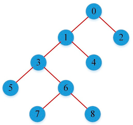
Figure 1.
Presentation of a simple classification and regression decision tree (CART).
To develop the CART model, the maximum tree depth was considered as five, which showed that the sample was recursively split five times. It also indicated that there are five levels below the root node. To avoid overfitting and deal with missing values, the authors pruned the tree using the “maximum surrogates” technique which eliminates bottom-level splits that do not substantially improve the accuracy of the tree. In order to control how the CART tree is constructed, two stopping rules, including the (1) minimum records in the parent branch and (2) minimum records in the child branch, were considered. The value of the former parameter was set as two, and it prevented a split if the number of records in the parent node to be divided was less than two. The former parameter was set as one, and it prevented a split if the number of records in any child branch created by the split was less than one. The authors used two parameters to determine the behavior of assembly that occurs during the boosting and bagging: (1) combining rule for continuous target, and (2) the number of component models for boosting and/or bagging. The authors used the mean of the predicted values from the base models to combine the ensemble values for the continuous target of this study. For boosting and bagging, the number of base models to build was set as 10. This number may improve the CART model accuracy and stability. To fine-tune the CART tree-building process, two advanced parameters were used: (1) minimum change in impurity and (2) overfit prevention set. The former parameter was used to create a new split in the tree and was set as 0.0001. The latter parameter was used to track errors during training to prevent the CART from modeling chance variation in the data. The percentage of records was set as 30.
CHAID is a widely used and non-binary decision tree, which was developed by Kass [84]. CHAID creates the decision tree using several sequential combinations and splits, based on a chi-square test. To avoid overfitting, which is one of the most common drawbacks of decision trees, it automatically prunes the tree. CHAID also produces a number of rules, whereby each has a confidence level (accuracy). The confidence level is defined as the ratio of records having the specific value for the target variable to the given values for the independent variables.
Similarly to the CART model, the same values were used for maximum tree depth, minimum records in parent branch, minimum records in child branch, combining rule for continues target, and the number of component models for boosting and/or bagging to develop the CHAID model. However, more settings were used to develop the CHAID decision tree model compared to the CART model. To fine-tune the CHAID tree-building process, five parameters were used: (1) significance level for splitting, (2) significance level for merging, (3) adjustment of significance values technique, (4) minimum change in expected cell frequencies, and (5) maximum iterations for convergence. The significance levels for splitting and merging were set as 0.05. To control the false-positive error rate, an adjustment of significance values technique known as the “Boferroni method” was used. In order to converge on the optimal estimate used in the chi-square test for a specific split, the minimum change in expected cell frequencies was used and set as 0.001. The last parameter specified the maximum number of iterations before stopping, whether convergence occurred or not. This parameter was set to 0.001.
Decision trees are regarded as unstable and high-variance models, which causes the trees to be prone to different generalization behavior with small changes in the training data [85]. The RF method can be used to avoid the abovementioned drawbacks. RF is a relatively new tree-based method and was developed by Breiman [86]. RF is an ensemble technique that produces more accurate prediction compared to other tree-based methods by merging a huge number of decision trees. RF uses a bagging technique to build each ensemble from different datasets. The bagging technique randomly selects from the space of decision trees and creates almost identical (low-diversity) predictions.
2.3. Artificial Neural Network
The artificial neural network (ANN) is a non-linear statistical data modeling technique for decision-making [87]. ANN is able to find patterns in data, or to unveil relations between input variables and the target variable. ANN is applied to different fields, such as function approximation, classification, and data processing. This technique uses a connectionist approach for computation. Mostly, an ANN can be viewed as an adaptive system that modifies its structure according to internal and external information which flows through the network during the learning stage. In ANN, the weights represent the connections of the biological neurons. An excitatory connection is shown by a positive weight, while an inhibitory connection is shown by a negative value. Typically, the ANN uses a multilayer perception (MLP) approximator which is a class of feed-forward ANN. MLP comprises at least three layers of nodes: an input layer, a hidden layer, and an output layer. Its multiple layers differentiate MLP from a linear perceptron. In fact, it can differentiate data that are not linearly separable [87].
The authors developed the ANN model through an MLP approximator which allowed for more complex associations at the possible cost of raising the training and scoring time. Moreover, the authors set the maximum number of minutes for the algorithm to run as 15. Once an ensemble model is created, this is the training time allowed for each component model of the ensemble. The authors used the mean of the predicted values from the base models to combine the ensemble values for the continuous target of this study. For boosting and bagging, the number of base models to build was set as 10. This number may enhance the model accuracy and stability. To control the options that do not fit neatly into other groups of setting, the authors used two parameters: (1) overfit prevention set and (2) missing values in predictors. The former is an independent set of data records used to track errors during training to prevent the method from modeling chance variation in the data. The percentage of records was set as 30. The latter specifies how to deal with missing values. The authors used the delete listwise approach, which eliminates records with missing values on predictors from model building.
2.4. Support Vector Machine
Support vector machine (SVM) is one of the most frequently used methods for regression and classification problems [88]. Several advantages of SVM are acknowledged in the literature. For example, this method can be effectively applied to high-dimensional and linearly non-separable datasets [89,90]. According to Cortes and Vapnik [91], statistical learning theory is the basic theory behind SVM. Several kernel functions, including linear, radial basis function, sigmoid and polynomial, also influence the performance of SVM [92]. The SVM aims to determine an ideal separation hyperplane that can distinguish two classes [92]. Furthermore, the SVM can reduce both the error (for training and testing datasets) and the complexity of model [93].
To develop the SVM model and data transformation in this study, the authors used the radial basis function (RBF) as the mathematical function. It is noteworthy to mention that the authors developed the SVM models using different kernel functions, including linear, radial basis function, sigmoid, and polynomial. Since the RBF resulted in higher accuracy compared to other kernels, the model developed using the RBF was used in this study. Additionally, a stopping criterion was used to determine when to stop the optimization algorithm. Values ranged from 1.0 × 10⁻¹ to 1.0 × 10⁻⁶. The authors used different values to run the SVM models. According to the results, the value of 1.0 × 10⁻³ was selected as the best since it resulted in the highest accuracy and lowest training time among stopping criterion values. A regularization parameter (C) was used to provide control of the trade-off between maximizing the margin and minimizing the training error term. C values ranged from 1–10. Because higher values of C may result in higher classification accuracy, the authors used the value of 10.
2.5. Case Study and Data Collection
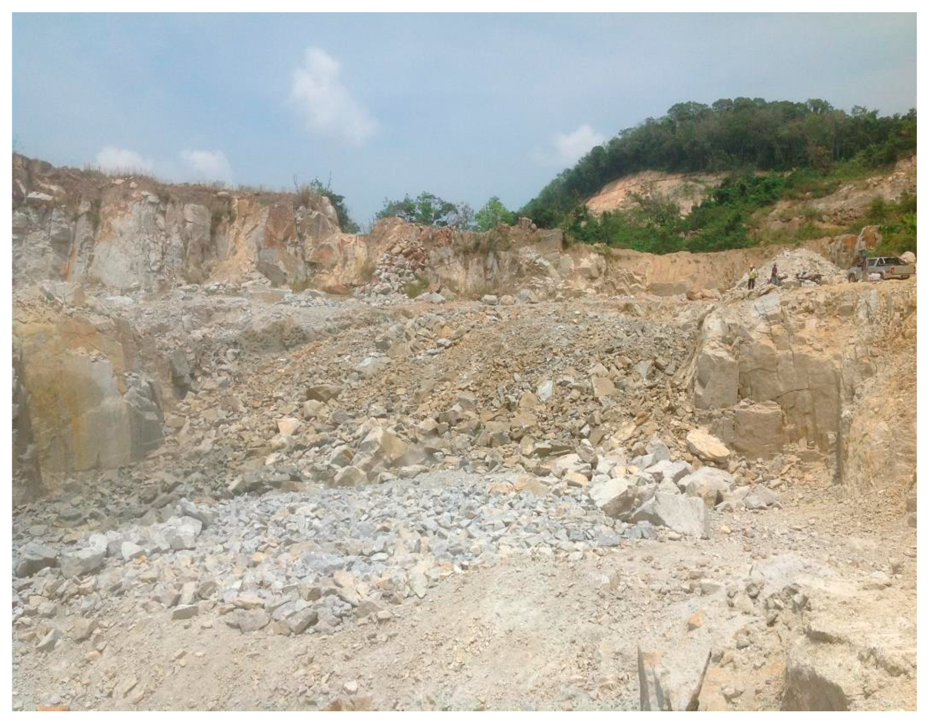
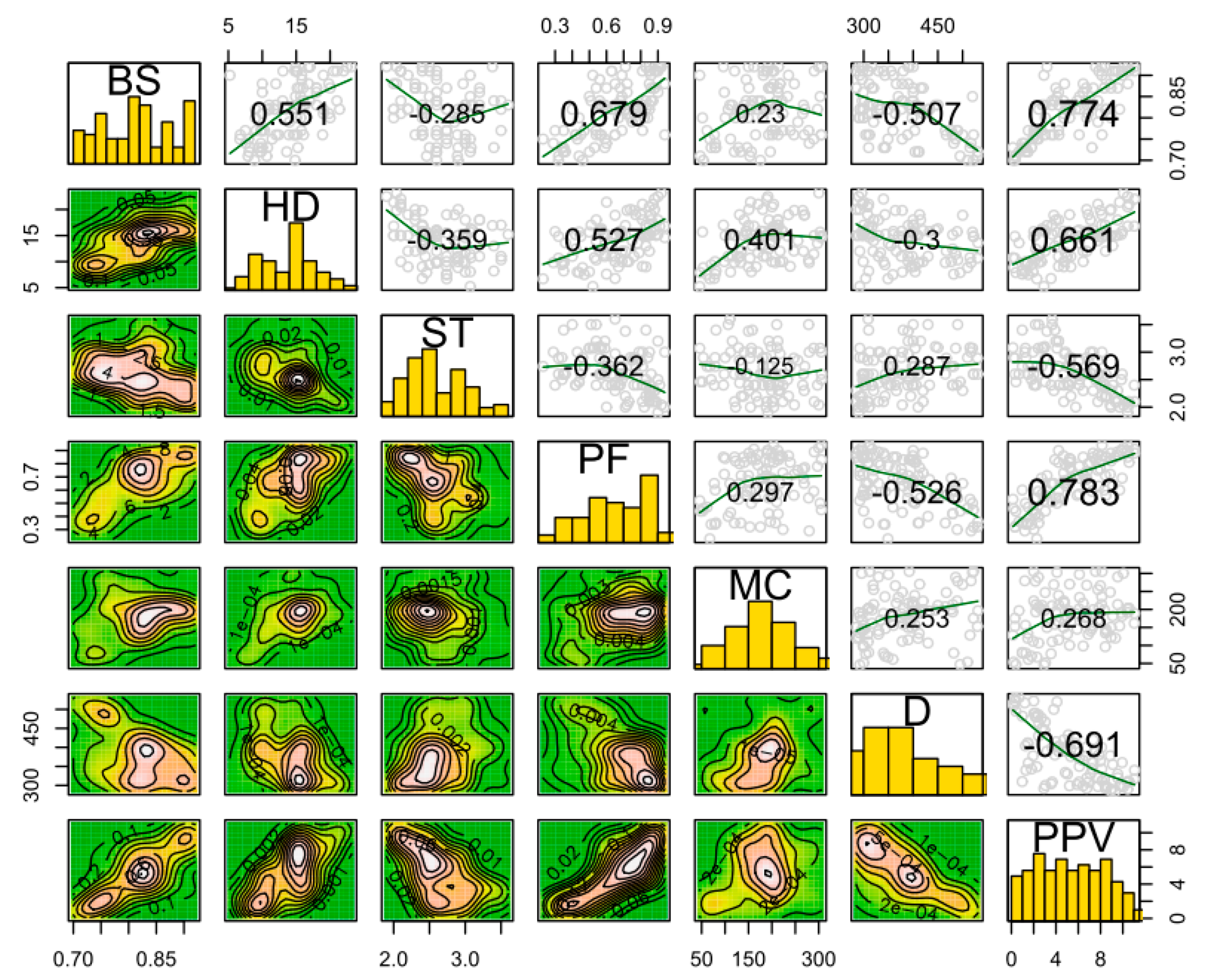
In this research, in order to have an interesting prediction purpose, an extensive dataset was collected from a mine containing explosive operations. A main view of the granite mine is shown in Figure 2. In general, explosive operations are common in this mine and are repeated at different intervals. The production capacity of this mine is about 500–700 thousand tons per year, and explosive operations use large quantities of explosives. The values of 856 kg to 9420 kg of explosives are usually used in holes with diameters between 76 mm and 89 mm. The highly explosive operations increased the danger in the mine. In this research, 102 operations were accurately measured and evaluated with all design details. Important parameters such as the burden, spacing, hole diameter, hole depth, total charge, number of holes, stemming length, maximum charge per delay, powder factor, sub-drilling, and distance from the blast-face, which help in determining PPV values were measured and recorded. Additionally, the Vibra ZEB seismographer was used for PPV recording. The distance from the seismograph to the explosion was about 280 m–530 m. According to the content given in Section 1 about the influence of various parameters, the importance of this parameter was determined by the effect of this phenomenon. In addition, previous research also made recommendations on the selection of effective parameters, the importance of each item, and design issues, which can be consulted for further information. Finally, the input data collected for the prediction and simulation purposes with the mathematical and probabilistic models are summarized in Table 3. Using this table, different ranges of recorded data can be seen. The relationships between the PPV and other input indicators are demonstrated in the correlation matrix plot (see Figure 3), which can be observed as the pairwise relationship between two indicators with corresponding correlation coefficients for each indicator. In the remaining sections, after input selection through the FS technique, five ML methods, i.e., RF, CART, CHAID, ANN, and SVM, are applied to predict PPV, and then the best PPV prediction model is selected and introduced.
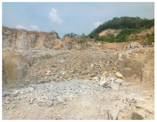
Figure 2.
A view of the investigated granite mine.

Table 3.
Recorded input and output data for prediction purposes.
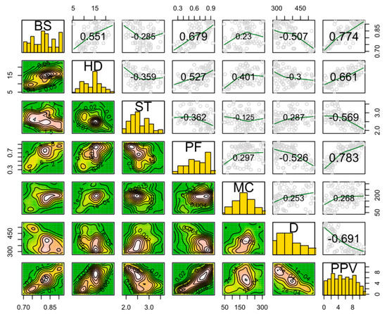
Figure 3.
Correlation matrix of input and output variables for all 102 blasting events.
3. Results
3.1. Input Selection Using FS Technique
An FS technique was used to reduce the dimensionality of the data and select the most important input variables. Table 4 shows the results obtained from the FS technique. The FS technique reduced the number of input variables from six to five. Thus, FS identified the maximum charge per delay (MC), hole depth (HD), stemming (ST), powder factor (PF), and distance (D) as the most important input variables. These variables were then used to develop five ML models to predict the PPV.

Table 4.
The importance value of the selected input variables using the feature selection (FS) technique.
3.2. Development of ML Models
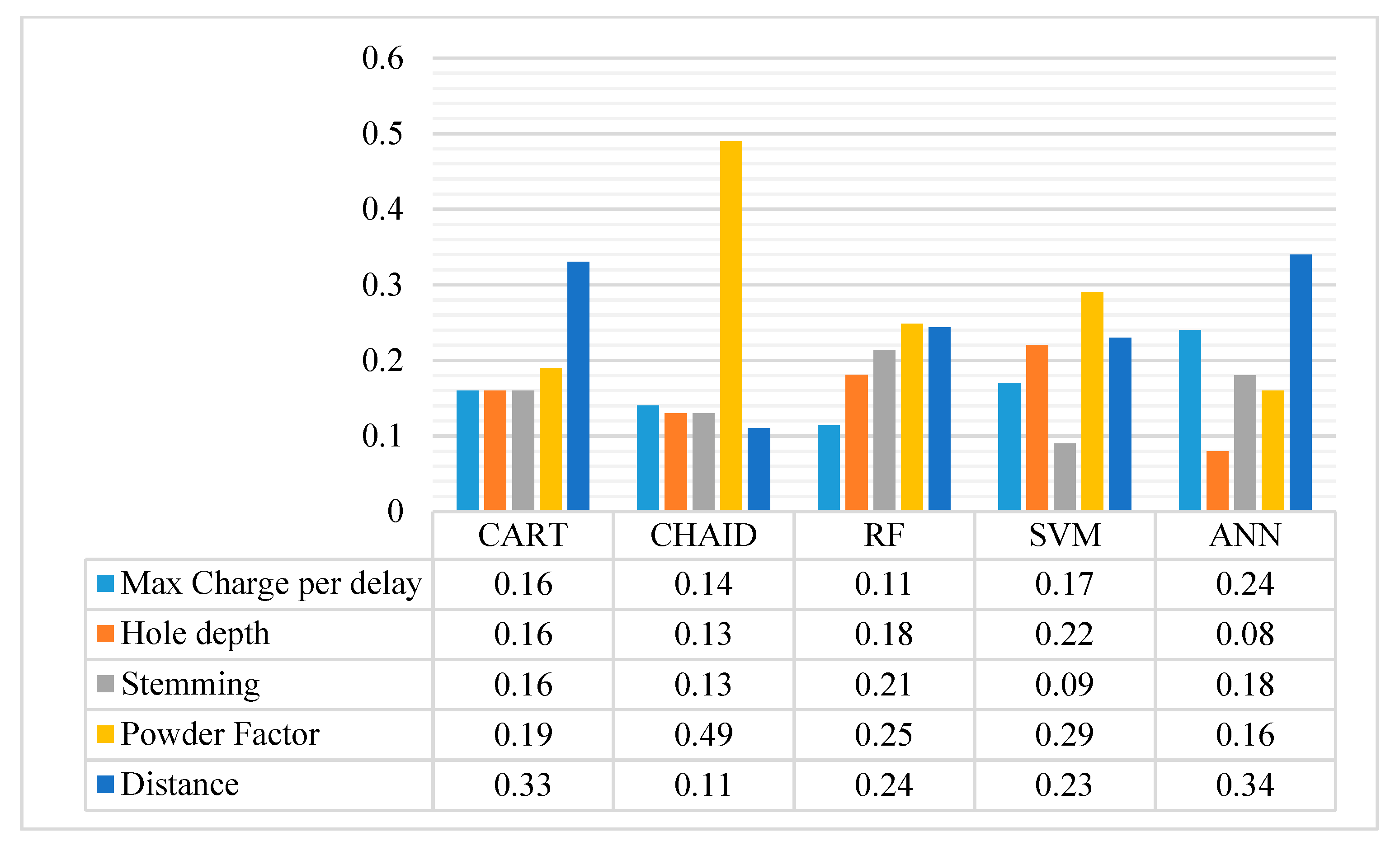
The authors of this study developed five ML models, namely, RF, CART, CHAID, SVM, and ANN. Each of these models was evaluated in terms of performance using four indices. These models also determined the importance of each input variable to predict the PPV. Thus, the authors compared the importance of each input variable across the developed models (Figure 4). According to the chart, PF was the most important variable to predict the PPV for the methods of CHAID, RF, and SVM. On the other hand, the methods of CART and ANN determined D as the most important variable. It is worth noting that RF uses an ensemble approach to develop the final tree; thus, the RF results may be more reliable than other decision tree methods.
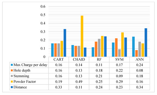
Figure 4.
Variable importance through the developed models.
3.3. Assessment of the Proposed Models
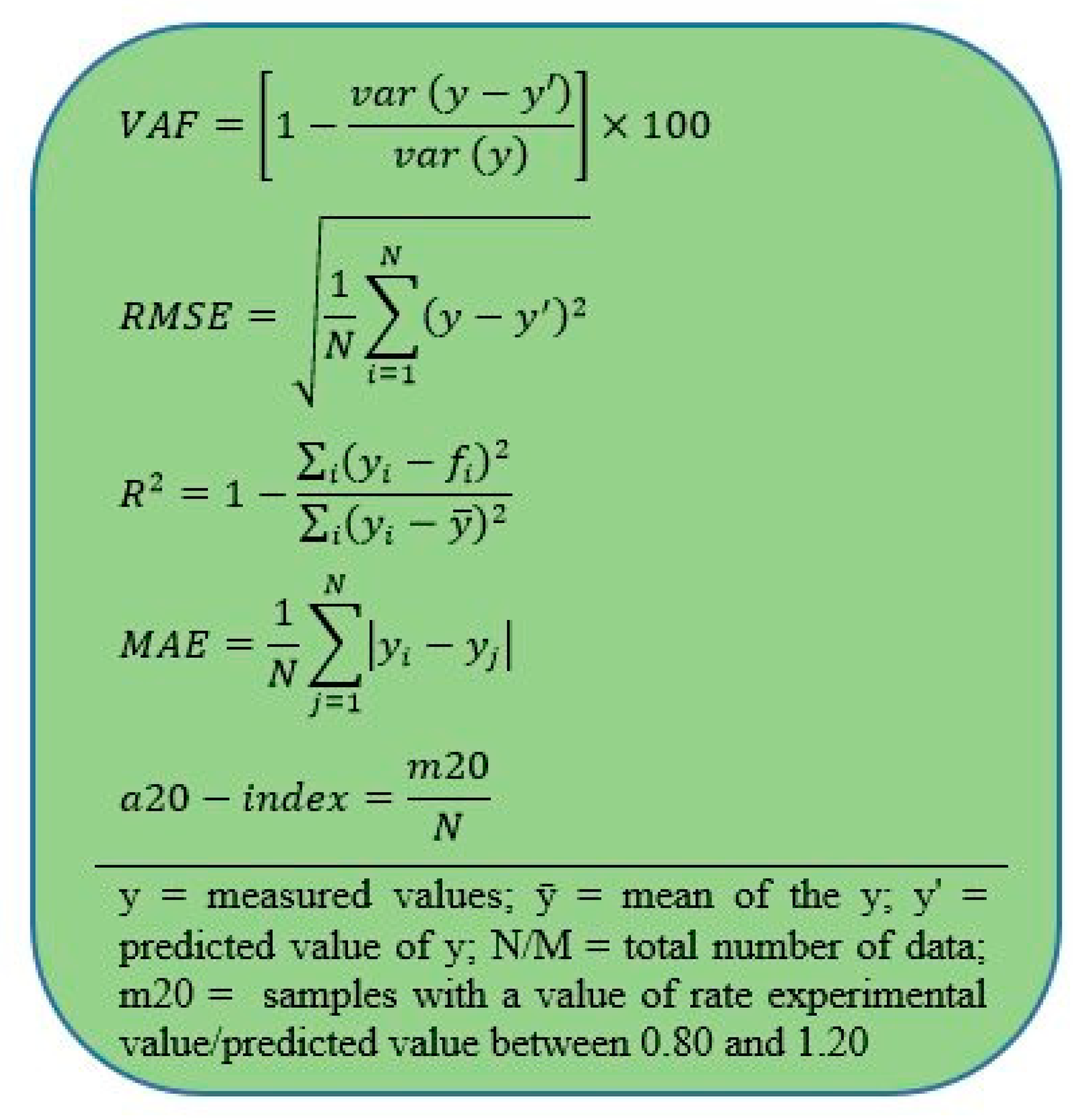
The present study used five performance indices to assess the performance of the models developed. These included coefficient of determination (R2), mean absolute error (MAE), root-mean-square error (RMSE), variance accounted for (VAF), and a20-index [32,40,41,42,44,94,95,96,97]. These indices were widely used in previous studies for the performance assessment of ML models. The computation formulas are presented in Figure 5.
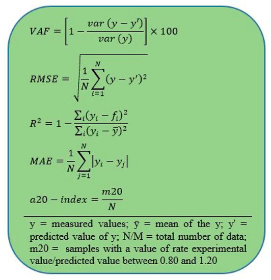
Figure 5.
Performance indices for evaluating the developed machine learning (ML) models.
This study also used a simple ranking system proposed by Zorlu et al. [86] to rank the performance of each proposed PPV prediction model. Before the model development, the authors split the data into training (70%) and testing (30%) datasets. For each dataset, this technique assigned a rank of five to the model that had the best value for each performance index, and then assigned a rank of one to the model that had the worst value for each performance index. The total performance rating of each model was then calculated by summing up its total rank of each dataset (Equation (1)). The authors also calculated the final rank of each model by summing up the training and testing dataset total ranks of the model. Table 5 shows the results of performance evaluation and the final ranking of each proposed model. Overall, the RF model obtained the highest final rank (41) by far, followed by ANN, CHAID, and SVM. CART achieved the lowest final rank (10). RF had the highest total rank (23) for the training dataset, while SVM and ANN had the highest total rank (21) for the testing dataset. The CART model had the lowest total rank for both training and testing datasets.
where i denotes the performance indices, and Ri is the model’s ranking for each performance index.

Table 5.
Obtained results of performance indices for all developed models in estimating PPV.
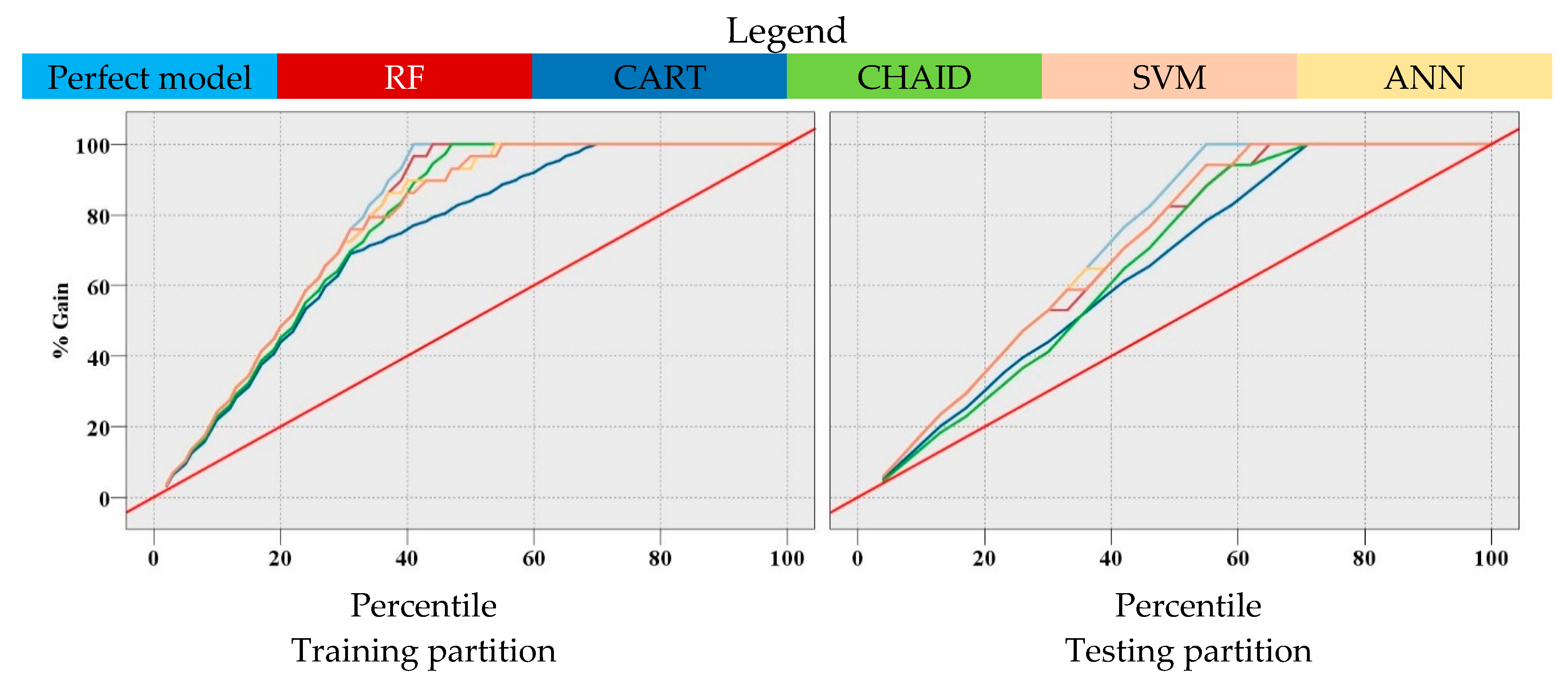
The performance of the proposed models was also evaluated using a gain chart, which is shown in Figure 6. A simple definition of gains is the proportion of total hits that occur in each percentile or increment. In the chart below, the diagonal red line denotes the at-chance model, the blue line (the higher line) denotes the perfect prediction model, and the other five lines in the middle represent the models that were developed in this study. Basically, higher lines indicate better models, specifically on the left side of the gain chart. The areas between each of the models and the red line show how much better the proposed models are compared to the at-chance model. Furthermore, the areas between each of the models and the perfect model show where the proposed models can be improved. It is worth noting that the aim of the developed models is to be as close to the perfect model as possible. The models also identified a PPV of greater than 5.59 mm/s as the best predictive value for the perfect model.

Figure 6.
Gain chart for comparing the accuracy of the developed models.
For the training dataset, as we went through 40% of the data, the at-chance model indicated that we correctly identified 40% of the samples which had a PPV of greater than 5.59 mm/s. The perfect model showed that we correctly identified 100% of the samples which had a PPV of greater than 5.59 mm/s. As we went through 44% of the data, the RF model showed that we identified 100% of the samples with the probability of a PPV of greater than 5.59 mm/s. As we went through 46% of the data, the CHAID model showed that we identified 100% of the samples with the probability of a PPV of greater than 5.59 mm/s. As we went through 54% of the data, the ANN model showed that we identified 100% of the samples with the probability of a PPV of greater than 5.59 mm/s. As we went through 55% of the data, the SVM model showed that we identified 100% of the samples with the probability of a PPV of greater than 5.59 mm/s. As we went through 68% of the data, the CART model showed that we identified 100% of the samples with the probability of a PPV of greater than 5.59 mm/s.
The gain chart illustrates that the performance of the RF model was better than other proposed models for the training dataset since the performance of this model was closer to the perfect model compared to the other proposed models. For the testing dataset, the ANN and SVM models performed slightly better than the RF model and other proposed models.
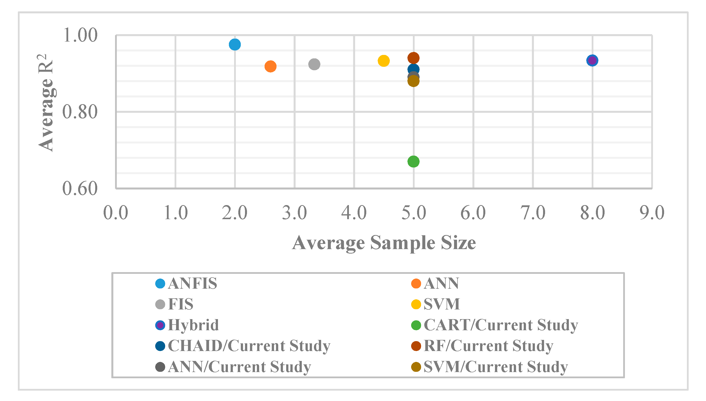
The authors provide a comparison between the achieved R2 values in previous studies that were listed in Table 1 and the current study. Figure 7 shows the average number of input variables and average R2 values for several types of models. This figure shows that the ANFIS models with two input variables obtained an average R2 value of 0.98, which was the highest value among other models. The ANFIS was followed by SVM and hybrid models (PSO–ANN and ICA–ANN) that had 4.5 and eight input variables on average and achieved an average R2 value of 0.93. In addition, ANN and FIS models that had 2.6 and 3.3 input variables on average could obtain an average R2 value of 0.92. Turning to this present study, the authors used a hybrid approach to develop several models using six input variables. The FS–RF model developed in this study showed a higher R2 compared to the previous hybrid models, including PSO–ANN and ICA–ANN, while a lower number of input variables were used to develop this model. The other models developed in this study achieved a lower R2 compared to the models previously developed.
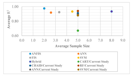
Figure 7.
Comparison of average R2 values and input variable numbers of the models developed in previous and current studies.
Comparing the results of this study with similar studies in terms of predictive techniques, it was found that the present study has some advantages. For example, concerning the study by Hasanipanah et al. [78], they only developed a CART model (one of the implemented techniques of this study) to predict PPV induced by blasting using MC and D parameters as inputs. In addition, Nam Bui et al. [98] developed a hybrid model of PSO and k-nearest neighbors (KNN) to estimate the blast-induced PPV. The database included 152 blasting events. Three different kernel functions were used to develop the KNN models. They used two input variables, including MC and D, for predicting PPV. The results of the PSO–KNN models were compared with RF and support vector regression (SVR) in terms of R2, RMSE, and MAE. The results of this study show that the R2 values of PSO–KNN (training = 0.982, testing = 0.977) was higher than RF (training = 0.996, testing = 0.953) and SVR (training = 0.973, testing = 0.944) models for both training and testing datasets. The difference between our study and the study by Bui et al. [98] is based on three aspects: (1) different input parameters, (2) different case study and type of rock mass and region, and (3) different predictive techniques. According to the above discussion, the methods presented in this study have a high level of originality and novelty in the field of blasting environmental issues.
4. Summary and Conclusions
This study set out with the aim of comparing the different ML techniques to predict ground vibration (PPV) due to quarry blasting. Thus, five methods, including RF, CART, CHAID, ANN, and SVM, were used. Before development of the models, an FS method was used to identify the most important input variables and reduce the dimensionality of the data. Concerning the variable importance, the results of the analysis of variable importance showed that the magnitudes of variable importance between the considered models differed. This indicates that these models identified the relationships between variables in a dissimilar manner. While RF showed a better performance for the training dataset compared to other methods used in this study, the ANN and SVM together obtained the highest rank for the testing dataset. The higher rank of RF for the training dataset shows that its flexibility, which is achieved by combining multiple decision trees, is particularly useful for predicting ground vibration. The performance of RF was significantly better than other tree-based regression models like CHAID and CART. This difference can be connected to the larger diversity among the learned trees of RF, which is a consequence of RF’s procedure for randomized splitting at nodes. Typically, ensemble regression models function better if there is notable diversity among the models [99]. However, the performance of CART was inferior to both RF and CHAID. It can be explained by the fact that CART models are more prone to overfitting, while RF and CHAID conceptually aim to reduce model variance and consequently avoid overfitting.
The aim of the FS techniques is not only increasing the model accuracy. The FS techniques also aim to reduce model dimensionality/complexity, training time, and overfitting risk [100]. In addition, these techniques may increase the model generalization ability [101]. It is worth mentioning that the FS techniques are heuristic, as they are just an indication of what may work well. The authors of this present study compared the predictive accuracies achieved from different models, with and without FS. It was found that the hybridization of FS and RF increased the R2 value, while this hybridization decreased the number of input variables. The results confirmed the effectiveness of FS technique employment before developing the RF model to predict the PPV.
The evaluation using the gain chart confirmed the results of performance indices. The RF performance for the training dataset was better than that for the testing dataset. In fact, the RF model correctly predicted 100% of the samples that had a PPV of greater than 5.59 mm/s when we went through 44% of the training dataset, while, for the testing dataset, the RF model correctly predicted 100% of the samples that had a PPV of greater than 5.59 mm/s when we went through 65% of data.
Better performance of RF over SVM and ANN was relatively unexpected, since both SVM and ANN use more advanced techniques compared to the RF to predict the target variable. The findings of this study suggest that RF can be used as an effective method to predict the PPV. Moreover, RF is a more powerful method compared to other decision tree methods to determine the importance of input variables, as the RF considers a huge number of trees (e.g., 100) and prevents the masking of the tree by another correlated input. However, caution must be taken when applying the results to other studies, since the present study used only five input variables, including MC, HD, ST, PF, and D. Future studies can develop the RF model to predict the PPV using more or different input variables.
Author Contributions
Formal analysis, H.Z.; conceptualization, D.J.A.; supervision, J.Z.; writing—review and editing, M.M.T., B.T.P., and D.J.A.; validation, V.V.H. All authors have read and agreed to the published version of the manuscript.
Funding
This work was financially supported by the National Natural Science Foundation Project of China (No. 41807259), the State Key Laboratory of Safety and Health for Metal Mines (No. 2017-JSKSSYS-04), the Project of Changsha Science and Technology Project (No. kc1809012), the Project for the Hunan Social Science Results Review Committee (No. XSP18YBC343), the Innovation-Driven Project of Central South University (2020CX040), and the Research Foundation of Education Bureau of Hunan Province, China (Nos. 18A381 and 18A295).
Conflicts of Interest
The authors declare no conflicts of interest.
Abbreviations
| ANFIS | Adaptive neuro-fuzzy inference system |
| ANN | Artificial neural network |
| CHAID | Chi-squared automatic interaction detection |
| CART | Classification and regression trees |
| R2 | Coefficient of determination |
| FS | Feature selection |
| FIS | Fuzzy inference system |
| GEP | Gene expression programming |
| GA | Genetic algorithm |
| GP | Genetic programming |
| ICA | Imperialism competitive algorithm |
| ML | Machine learning |
| MAE | Mean absolute error |
| MLP | Multilayer perception |
| PSO | Particle swarm optimization |
| PPV | Peak particle velocity |
| QUEST | Quick, unbiased, efficient, and statistical tree |
| RBF | Radial basis function |
| RF | Random forest |
| RMSE | Root mean square error |
| SVM | Support vector machine |
| VAF | Variance accounted for |
References
- Khandelwal, M.; Kumar, D.L.; Yellishetty, M. Application of soft computing to predict blast-induced ground vibration. Eng. Comput. 2011, 27, 117–125. [Google Scholar] [CrossRef]
- Ebrahimi, E.; Monjezi, M.; Khalesi, M.R.; Armaghani, D.J. Prediction and optimization of back-break and rock fragmentation using an artificial neural network and a bee colony algorithm. Bull. Eng. Geol. Environ. 2016, 75, 27–36. [Google Scholar] [CrossRef]
- Dindarloo, S.R. Prediction of blast-induced ground vibrations via genetic programming. Int. J. Min. Sci. Technol. 2015, 25, 1011–1015. [Google Scholar] [CrossRef]
- Armaghani, D.J.; Hajihassani, M.; Mohamad, E.T.; Marto, A.; Noorani, S.A. Blasting-induced flyrock and ground vibration prediction through an expert artificial neural network based on particle swarm optimization. Arab. J. Geosci. 2014, 7, 5383–5396. [Google Scholar] [CrossRef]
- Hajihassani, M.; Jahed Armaghani, D.; Sohaei, H.; Tonnizam Mohamad, E.; Marto, A. Prediction of airblast-overpressure induced by blasting using a hybrid artificial neural network and particle swarm optimization. Appl. Acoust. 2014, 80, 57–67. [Google Scholar] [CrossRef]
- Armaghani, D.J.; Hajihassani, M.; Sohaei, H.; Mohamad, E.T.; Marto, A.; Motaghedi, H.; Moghaddam, M.R. Neuro-fuzzy technique to predict air-overpressure induced by blasting. Arab. J. Geosci. 2015, 8, 10937–10950. [Google Scholar] [CrossRef]
- Tonnizam Mohamad, E.; Hajihassani, M.; Jahed Armaghani, D.; Marto, A. Simulation of blasting-induced air overpressure by means of Artificial Neural Networks. Int. Rev. Model. Simul. 2012, 5, 2501–2506. [Google Scholar]
- Mohamad, E.T.; Armaghani, D.J.; Noorani, S.A.; Saad, R.; Alvi, S.V.; Abad, N.K. Prediction of flyrock in boulder blasting using artificial neural network. Electron. J. Geotech. Eng. 2012, 17, 2585–2595. [Google Scholar]
- Khandelwal, M.; Singh, T.N. Prediction of blast-induced ground vibration using artificial neural network. Int. J. Rock Mech. Min. Sci. 2009, 46, 1214–1222. [Google Scholar] [CrossRef]
- Hasanipanah, M.; Bakhshandeh Amnieh, H.; Khamesi, H.; Jahed Armaghani, D.; Bagheri Golzar, S.; Shahnazar, A. Prediction of an environmental issue of mine blasting: An imperialistic competitive algorithm-based fuzzy system. Int. J. Environ. Sci. Technol. 2018, 15, 551–560. [Google Scholar] [CrossRef]
- Monjezi, M.; Ahmadi, M.; Sheikhan, M.; Bahrami, A.; Salimi, A.R. Predicting blast-induced ground vibration using various types of neural networks. Soil Dyn. Earthq. Eng. 2010, 30, 1233–1236. [Google Scholar] [CrossRef]
- Armaghani, D.J.; Momeni, E.; Abad, S.V.A.N.K.; Khandelwal, M. Feasibility of ANFIS model for prediction of ground vibrations resulting from quarry blasting. Environ. Earth Sci. 2015, 74, 2845–2860. [Google Scholar] [CrossRef]
- Singh, T.N.; Singh, V. An intelligent approach to prediction and control ground vibration in mines. Geotech. Geol. Eng. 2005, 23, 249–262. [Google Scholar] [CrossRef]
- Toraño, J.; Ramírez-Oyanguren, P.; Rodríguez, R.; Diego, I. Analysis of the environmental effects of ground vibrations produced by blasting in quarries. Int. J. Min. Reclam. Environ. 2006, 20, 249–266. [Google Scholar] [CrossRef]
- Ozer, U.; Kahriman, A.; Aksoy, M.; Adiguzel, D.; Karadogan, A. The analysis of ground vibrations induced by bench blasting at Akyol quarry and practical blasting charts. Environ. Geol. 2008, 54, 737–743. [Google Scholar] [CrossRef]
- Faramarzi, F.; Farsangi, M.A.E.; Mansouri, H. Simultaneous investigation of blast induced ground vibration and airblast effects on safety level of structures and human in surface blasting. Int. J. Min. Sci. Technol. 2014, 24, 663–669. [Google Scholar] [CrossRef]
- Duvall, W.I.; Petkof, B. Spherical Propagation of Explosion-Generated Strain Pulses in Rock; USBM: Washington, DC, USA, 1959.
- Dowding, C.H. Suggested Method for Blast Vibration Monitoring. Int. J. Rock Mech. Min. Sci. Geomech. Abstr. 1992, 29, 145–156. [Google Scholar] [CrossRef]
- Indian Standard. Criteria for Safety and Design of Structures Subjected to under Ground Blast; No 15-6922; ISI: Karnataka, India, 1973.
- Kahriman, A. Analysis of ground vibrations caused by bench blasting at can open-pit lignite mine in Turkey. Environ. Geol. 2002, 41, 653–661. [Google Scholar] [CrossRef]
- Ambraseys, N.N.; Hendron, A.J. Dynamic Behaviour of Rock Masses; John Wiley & Sons: Hoboken, NJ, USA, 1968. [Google Scholar]
- Davies, B.; Farmer, I.W.; Attewell, P.B. Ground vibration from shallow sub-surface blasts. Engineer 1964, 217, 5644. [Google Scholar]
- Langefors, U.; Kihlstrom, B. The Modern Technique of Rock Blasting; Wiley: New York, NY, USA, 1963. [Google Scholar]
- Roy, P. Putting ground vibration predictions into practice. Colliery Guard. 1993, 241, 63–67. [Google Scholar]
- Khandelwal, M.; Singh, T.N. Evaluation of blast-induced ground vibration predictors. Soil Dyn. Earthq. Eng. 2007, 27, 116–125. [Google Scholar] [CrossRef]
- Verma, A.K.; Singh, T.N. Intelligent systems for ground vibration measurement: A comparative study. Eng. Comput. 2011, 27, 225–233. [Google Scholar] [CrossRef]
- Verma, A.K.; Singh, T.N. A neuro-fuzzy approach for prediction of longitudinal wave velocity. Neural Comput. Appl. 2013, 22, 1685–1693. [Google Scholar] [CrossRef]
- Hudaverdi, T. Application of multivariate analysis for prediction of blast-induced ground vibrations. Soil Dyn. Earthq. Eng. 2012, 43, 300–308. [Google Scholar] [CrossRef]
- Hajihassani, M.; Jahed Armaghani, D.; Marto, A.; Tonnizam Mohamad, E. Ground vibration prediction in quarry blasting through an artificial neural network optimized by imperialist competitive algorithm. Bull. Eng. Geol. Environ. 2014, 74, 873–886. [Google Scholar] [CrossRef]
- Monjezi, M.; Baghestani, M.; Shirani Faradonbeh, R.; Pourghasemi Saghand, M.; Jahed Armaghani, D. Modification and prediction of blast-induced ground vibrations based on both empirical and computational techniques. Eng. Comput. 2016, 32, 717–728. [Google Scholar] [CrossRef]
- Mohamed, M.T. Performance of fuzzy logic and artificial neural network in prediction of ground and air vibrations. Int. J. Rock Mech. Min. Sci. 2011, 48, 845. [Google Scholar] [CrossRef]
- Xu, H.; Zhou, J.; Asteris, P.G.; Jahed Armaghani, D.; Tahir, M.M. Supervised Machine Learning Techniques to the Prediction of Tunnel Boring Machine Penetration Rate. Appl. Sci. 2019, 9, 3715. [Google Scholar] [CrossRef]
- Apostolopoulou, M.; Armaghani, D.J.; Bakolas, A.; Douvika, M.G.; Moropoulou, A.; Asteris, P.G. Compressive strength of natural hydraulic lime mortars using soft computing techniques. Procedia Struct. Integr. 2019, 17, 914–923. [Google Scholar] [CrossRef]
- Gordan, B.; Jahed Armaghani, D.; Hajihassani, M.; Monjezi, M. Prediction of seismic slope stability through combination of particle swarm optimization and neural network. Eng. Comput. 2016, 32, 85–97. [Google Scholar] [CrossRef]
- Zhou, J.; Aghili, N.; Ghaleini, E.N.; Bui, D.T.; Tahir, M.M.; Koopialipoor, M. A Monte Carlo simulation approach for effective assessment of flyrock based on intelligent system of neural network. Eng. Comput. 2019. [Google Scholar] [CrossRef]
- Zhou, J.; Koopialipoor, M.; Murlidhar, B.R.; Fatemi, S.A.; Tahir, M.M.; Armaghani, D.J.; Li, C. Use of Intelligent Methods to Design Effective Pattern Parameters of Mine Blasting to Minimize Flyrock Distance. Nat. Resour. Res. 2019. [Google Scholar] [CrossRef]
- Koopialipoor, M.; Murlidhar, B.R.; Hedayat, A.; Armaghani, D.J.; Gordan, B.; Mohamad, E.T. The use of new intelligent techniques in designing retaining walls. Eng. Comput. 2019, 36, 283–294. [Google Scholar] [CrossRef]
- Guo, H.; Zhou, J.; Koopialipoor, M.; Armaghani, D.J.; Tahir, M.M. Deep neural network and whale optimization algorithm to assess flyrock induced by blasting. Eng. Comput. 2019. [Google Scholar] [CrossRef]
- Armaghani, D.J.; Koopialipoor, M.; Marto, A.; Yagiz, S. Application of several optimization techniques for estimating TBM advance rate in granitic rocks. J. Rock Mech. Geotech. Eng. 2019, 11, 779–789. [Google Scholar] [CrossRef]
- Harandizadeh, H.; Armaghani, D.J.; Khari, M. A new development of ANFIS–GMDH optimized by PSO to predict pile bearing capacity based on experimental datasets. Eng. Comput. 2019. [Google Scholar] [CrossRef]
- Khari, M.; Dehghanbandaki, A.; Motamedi, S.; Armaghani, D.J. Computational estimation of lateral pile displacement in layered sand using experimental data. Measurement 2019, 146, 110–118. [Google Scholar] [CrossRef]
- Shao, Z.; Armaghani, D.J.; Bejarbaneh, B.Y.; Mu’azu, M.A.; Mohamad, E.T. Estimating the Friction Angle of Black Shale Core Specimens with Hybrid-ANN Approaches. Measurement 2019, 145, 744–755. [Google Scholar] [CrossRef]
- Chen, W.; Sarir, P.; Bui, X.-N.; Nguyen, H.; Tahir, M.M.; Armaghani, D.J. Neuro-genetic, neuro-imperialism and genetic programing models in predicting ultimate bearing capacity of pile. Eng. Comput. 2019. [Google Scholar] [CrossRef]
- Hajihassani, M.; Abdullah, S.S.; Asteris, P.G.; Armaghani, D.J. A Gene Expression Programming Model for Predicting Tunnel Convergence. Appl. Sci. 2019, 9, 4650. [Google Scholar] [CrossRef]
- Zhou, J.; Li, X.; Mitri, H.S. Evaluation method of rockburst: State-of-the-art literature review. Tunn. Undergr. Space Technol. 2018, 81, 632–659. [Google Scholar] [CrossRef]
- Zhou, J.; Li, E.; Yang, S.; Wang, M.; Shi, X.; Yao, S.; Mitri, H.S. Slope stability prediction for circular mode failure using gradient boosting machine approach based on an updated database of case histories. Saf. Sci. 2019, 118, 505–518. [Google Scholar] [CrossRef]
- Wang, M.; Shi, X.; Zhou, J.; Qiu, X. Multi-planar detection optimization algorithm for the interval charging structure of large-diameter longhole blasting design based on rock fragmentation aspects. Eng. Optim. 2018, 50, 2177–2191. [Google Scholar] [CrossRef]
- Zhou, J.; Li, E.; Wei, H.; Li, C.; Qiao, Q.; Armaghani, D.J. Random Forests and Cubist Algorithms for Predicting Shear Strengths of Rockfill Materials. Appl. Sci. 2019, 9, 1621. [Google Scholar] [CrossRef]
- Zhou, J.; Li, E.; Wang, M.; Chen, X.; Shi, X.; Jiang, L. Feasibility of Stochastic Gradient Boosting Approach for Evaluating Seismic Liquefaction Potential Based on SPT and CPT Case Histories. J. Perform. Constr. Facil. 2019, 33, 4019024. [Google Scholar] [CrossRef]
- Asteris, P.G.; Mokos, V.G. Concrete compressive strength using artificial neural networks. Neural Comput. Appl. 2019. [Google Scholar] [CrossRef]
- Huang, L.; Asteris, P.G.; Koopialipoor, M.; Armaghani, D.J.; Tahir, M.M. Invasive Weed Optimization Technique-Based ANN to the Prediction of Rock Tensile Strength. Appl. Sci. 2019, 9, 5372. [Google Scholar] [CrossRef]
- Apostolopoulour, M.; Douvika, M.G.; Kanellopoulos, I.N.; Moropoulou, A.; Asteris, P.G. Prediction of Compressive Strength of Mortars using Artificial Neural Networks. In Proceedings of the 1st International Conference TMM_CH, Transdisciplinary Multispectral Modelling and Cooperation for the Preservation of Cultural Heritage, Athens, Greece, 10–13 October 2018; pp. 10–13. [Google Scholar]
- Zhou, J.; Li, X.; Shi, X. Long-term prediction model of rockburst in underground openings using heuristic algorithms and support vector machines. Saf. Sci. 2012, 50, 629–644. [Google Scholar] [CrossRef]
- Zhou, J.; Li, X.B.; Mitri, H.S. Classification of rockburst in underground projects: Comparison of ten supervised learning methods. J. Comput. Civ. Eng. 2016, 30, 04016003. [Google Scholar] [CrossRef]
- Sarir, P.; Chen, J.; Asteris, P.G.; Armaghani, D.J.; Tahir, M.M. Developing GEP tree-based, neuro-swarm, and whale optimization models for evaluation of bearing capacity of concrete-filled steel tube columns. Eng. Comput. 2019. [Google Scholar] [CrossRef]
- Yang, H.Q.; Xing, S.G.; Wang, Q.; Li, Z. Model test on the entrainment phenomenon and energy conversion mechanism of flow-like landslides. Eng. Geol. 2018, 239, 119–125. [Google Scholar] [CrossRef]
- Yang, H.Q.; Zeng, Y.Y.; Lan, Y.F.; Zhou, X.P. Analysis of the excavation damaged zone around a tunnel accounting for geostress and unloading. Int. J. Rock Mech. Min. Sci. 2014, 69, 59–66. [Google Scholar] [CrossRef]
- Liu, B.; Yang, H.; Karekal, S. Effect of Water Content on Argillization of Mudstone During the Tunnelling process. Rock Mech. Rock Eng. 2019. [Google Scholar] [CrossRef]
- Yang, H.; Liu, J.; Liu, B. Investigation on the cracking character of jointed rock mass beneath TBM disc cutter. Rock Mech. Rock Eng. 2018, 51, 1263–1277. [Google Scholar] [CrossRef]
- Yang, H.Q.; Li, Z.; Jie, T.Q.; Zhang, Z.Q. Effects of joints on the cutting behavior of disc cutter running on the jointed rock mass. Tunn. Undergr. Space Technol. 2018, 81, 112–120. [Google Scholar] [CrossRef]
- Armaghani, D.J.; Hatzigeorgiou, G.D.; Karamani, C.; Skentou, A.; Zoumpoulaki, I.; Asteris, P.G. Soft computing-based techniques for concrete beams shear strength. Procedia Struct. Integr. 2019, 17, 924–933. [Google Scholar] [CrossRef]
- Chen, H.; Asteris, P.G.; Jahed Armaghani, D.; Gordan, B.; Pham, B.T. Assessing Dynamic Conditions of the Retaining Wall: Developing Two Hybrid Intelligent Models. Appl. Sci. 2019, 9, 1042. [Google Scholar] [CrossRef]
- Asteris, P.G.; Nikoo, M. Artificial bee colony-based neural network for the prediction of the fundamental period of infilled frame structures. Neural Comput. Appl. 2019, 31, 4837–4847. [Google Scholar] [CrossRef]
- Asteris, P.G.; Nozhati, S.; Nikoo, M.; Cavaleri, L.; Nikoo, M. Krill herd algorithm-based neural network in structural seismic reliability evaluation. Mech. Adv. Mater. Struct. 2019, 26, 1146–1153. [Google Scholar] [CrossRef]
- Asteris, P.; Roussis, P.; Douvika, M. Feed-forward neural network prediction of the mechanical properties of sandcrete materials. Sensors 2017, 17, 1344. [Google Scholar] [CrossRef]
- Cavaleri, L.; Asteris, P.G.; Psyllaki, P.P.; Douvika, M.G.; Skentou, A.D.; Vaxevanidis, N.M. Prediction of Surface Treatment Effects on the Tribological Performance of Tool Steels Using Artificial Neural Networks. Appl. Sci. 2019, 9, 2788. [Google Scholar] [CrossRef]
- Khandelwal, M.; Singh, T.N. Prediction of blast induced ground vibrations and frequency in opencast mine: A neural network approach. J. Sound Vib. 2006, 289, 711–725. [Google Scholar] [CrossRef]
- Monjezi, M.; Ghafurikalajahi, M.; Bahrami, A. Prediction of blast-induced ground vibration using artificial neural networks. Tunn. Undergr. Space Technol. 2011, 26, 46–50. [Google Scholar] [CrossRef]
- Fişne, A.; Kuzu, C.; Hüdaverdi, T. Prediction of environmental impacts of quarry blasting operation using fuzzy logic. Environ. Monit. Assess. 2011, 174, 461–470. [Google Scholar] [CrossRef]
- Iphar, M.; Yavuz, M.; Ak, H. Prediction of ground vibrations resulting from the blasting operations in an open-pit mine by adaptive neuro-fuzzy inference system. Environ. Geol. 2008, 56, 97–107. [Google Scholar] [CrossRef]
- Mohamadnejad, M.; Gholami, R.; Ataei, M. Comparison of intelligence science techniques and empirical methods for prediction of blasting vibrations. Tunn. Undergr. Space Technol. 2012, 28, 238–244. [Google Scholar] [CrossRef]
- Li, D.T.; Yan, J.L.; Zhang, L. Prediction of blast-induced ground vibration using support vector machine by tunnel excavation. Appl. Mech. Mater. 2012, 170, 1414–1418. [Google Scholar] [CrossRef]
- Ghasemi, E.; Ataei, M.; Hashemolhosseini, H. Development of a fuzzy model for predicting ground vibration caused by rock blasting in surface mining. J. Vib. Control 2013, 19, 755–770. [Google Scholar] [CrossRef]
- Monjezi, M.; Hasanipanah, M.; Khandelwal, M. Evaluation and prediction of blast-induced ground vibration at Shur River Dam, Iran, by artificial neural network. Neural Comput. Appl. 2013, 22, 1637–1643. [Google Scholar] [CrossRef]
- Hasanipanah, M.; Monjezi, M.; Shahnazar, A.; Armaghani, D.J.; Farazmand, A. Feasibility of indirect determination of blast induced ground vibration based on support vector machine. Measurement 2015, 75, 289–297. [Google Scholar] [CrossRef]
- Dindarloo, S.R. Peak particle velocity prediction using support vector machines: A surface blasting case study. J. S. Afr. Inst. Min. Metall. 2015, 115, 637–643. [Google Scholar] [CrossRef]
- Hajihassani, M.; Jahed Armaghani, D.; Monjezi, M.; Mohamad, E.T.; Marto, A. Blast-induced air and ground vibration prediction: A particle swarm optimization-based artificial neural network approach. Environ. Earth Sci. 2015, 74, 2799–2817. [Google Scholar] [CrossRef]
- Hasanipanah, M.; Faradonbeh, R.S.; Amnieh, H.B.; Armaghani, D.J.; Monjezi, M. Forecasting blast-induced ground vibration developing a CART model. Eng. Comput. 2017, 33, 307–316. [Google Scholar] [CrossRef]
- Armaghani, D.J.; Hasanipanah, M.; Amnieh, H.B.; Mohamad, E.T. Feasibility of ICA in approximating ground vibration resulting from mine blasting. Neural Comput. Appl. 2018, 29, 457–465. [Google Scholar] [CrossRef]
- Shirani Faradonbeh, R.; Jahed Armaghani, D.; Abd Majid, M.Z.; MD Tahir, M.; Ramesh Murlidhar, B.; Monjezi, M.; Wong, H.M. Prediction of ground vibration due to quarry blasting based on gene expression programming: A new model for peak particle velocity prediction. Int. J. Environ. Sci. Technol. 2016, 13, 1453–1464. [Google Scholar] [CrossRef]
- Shahnazar, A.; Nikafshan Rad, H.; Hasanipanah, M.; Tahir, M.M.; Jahed Armaghani, D.; Ghoroqi, M. A new developed approach for the prediction of ground vibration using a hybrid PSO-optimized ANFIS-based model. Environ. Earth Sci. 2017, 76, 527. [Google Scholar] [CrossRef]
- Ghoraba, S.; Monjezi, M.; Talebi, N.; Armaghani, D.J.; Moghaddam, M.R. Estimation of ground vibration produced by blasting operations through intelligent and empirical models. Environ. Earth Sci. 2016, 75, 1137. [Google Scholar] [CrossRef]
- Breiman, L.; Friedman, J.; Olshen, R.; Stone, C. Classification and regression trees. Wadsworth Int. Group 1984, 37, 237–251. [Google Scholar]
- Kass, G.V. An exploratory technique for investigating large quantities of categorical data. J. R. Stat. Soc. Ser. C Appl. Stat. 1980, 29, 119–127. [Google Scholar] [CrossRef]
- Brown, G. Ensemble Learning. In Encyclopedia of Machine Learning; Springer: Boston, MA, USA, 2010; pp. 312–320. [Google Scholar]
- Breiman, L. Random forests. Mach. Learn. 2001, 45, 5–32. [Google Scholar] [CrossRef]
- Cybenko, G. Approximation by superpositions of a sigmoidal function. Math. Control. Signals Syst. 1989, 2, 303–314. [Google Scholar] [CrossRef]
- Vapnik, V.; Vapnik, V. Statistical Learning Theory; Wiley: New York, NY, USA, 1998; pp. 156–160. [Google Scholar]
- Kavzoglu, T.; Sahin, E.K.; Colkesen, I. Landslide susceptibility mapping using GIS-based multi-criteria decision analysis, support vector machines, and logistic regression. Landslides 2014, 11, 425–439. [Google Scholar] [CrossRef]
- Hasanipanah, M.; Shahnazar, A.; Bakhshandeh Amnieh, H.; Jahed Armaghani, D. Prediction of air-overpressure caused by mine blasting using a new hybrid PSO–SVR model. Eng. Comput. 2017, 33, 23–31. [Google Scholar] [CrossRef]
- Cortes, C.; Vapnik, V. Support-vector networks. Mach. Learn. 1995, 20, 273–297. [Google Scholar] [CrossRef]
- Hong, H.; Pradhan, B.; Bui, D.T.; Xu, C.; Youssef, A.M.; Chen, W. Comparison of four kernel functions used in support vector machines for landslide susceptibility mapping: A case study at Suichuan area (China). Geomat. Nat. Hazards Risk 2017, 8, 544–569. [Google Scholar] [CrossRef]
- Kalantar, B.; Pradhan, B.; Naghibi, S.A.; Motevalli, A.; Mansor, S. Assessment of the effects of training data selection on the landslide susceptibility mapping: A comparison between support vector machine (SVM), logistic regression (LR) and artificial neural networks (ANN). Geomat. Nat. Hazards Risk 2018, 9, 49–69. [Google Scholar] [CrossRef]
- Toghroli, A.; Mohammadhassani, M.; Suhatril, M.; Shariati, M.; Ibrahim, Z. Prediction of shear capacity of channel shear connectors using the ANFIS model. Steel Compos. Struct. 2014, 17, 623–639. [Google Scholar] [CrossRef]
- Asteris, P.G.; Apostolopoulou, M.; Skentou, A.D.; Moropoulou, A. Application of artificial neural networks for the prediction of the compressive strength of cement-based mortars. Comput. Concr. 2019, 24, 329–345. [Google Scholar]
- Khari, M.; Armaghani, D.J.; Dehghanbanadaki, A. Prediction of Lateral Deflection of Small-Scale Piles Using Hybrid PSO–ANN Model. Arab. J. Sci. Eng. 2019. [Google Scholar] [CrossRef]
- Asteris, P.G.; Tsaris, A.K.; Cavaleri, L.; Repapis, C.C.; Papalou, A.; Di Trapani, F.; Karypidis, D.F. Prediction of the fundamental period of infilled RC frame structures using artificial neural networks. Comput. Intell. Neurosci. 2016, 2016, 20. [Google Scholar] [CrossRef]
- Bui, X.-N.; Jaroonpattanapong, P.; Nguyen, H.; Tran, Q.-H.; Long, N.Q. A novel Hybrid Model for predicting Blast-induced Ground Vibration Based on k-nearest neighbors and particle Swarm optimization. Sci. Rep. 2019, 9, 1–14. [Google Scholar] [CrossRef]
- Kuncheva, L.I.; Whitaker, C.J. Measures of diversity in classifier ensembles and their relationship with the ensemble accuracy. Mach. Learn. 2003, 51, 181–207. [Google Scholar] [CrossRef]
- Guyon, I.; Elisseeff, A. An introduction to variable and feature selection. J. Mach. Learn. Res. 2003, 3, 1157–1182. [Google Scholar]
- Cortés, G.; Benitez, M.C.; García, L.; Álvarez, I.; Ibanez, J.M. A comparative study of dimensionality reduction algorithms applied to volcano-seismic signals. IEEE J. Sel. Top. Appl. Earth Obs. Remote Sens. 2015, 9, 253–263. [Google Scholar] [CrossRef]
© 2020 by the authors. Licensee MDPI, Basel, Switzerland. This article is an open access article distributed under the terms and conditions of the Creative Commons Attribution (CC BY) license (http://creativecommons.org/licenses/by/4.0/).


