Abstract
Recent years have witnessed significant advances in single image deblurring due to the increasing popularity of electronic imaging equipment. Most existing blind image deblurring algorithms focus on designing distinctive image priors for blur kernel estimation, which usually play regularization roles in deconvolution formulation. However, little research effort has been devoted to the relative scale ambiguity between the latent image and the blur kernel. The well-known normalization constraint, i.e., fixing the sum of all the kernel weights to be one, is commonly selected to remove this ambiguity. In contrast to this arbitrary choice, we in this paper introduce the -norm normalization constraint on the blur kernel associated with a hyper-Laplacian prior. We show that the employed hyper-Laplacian regularizer can be transformed into a joint regularized prior based on a scale factor. We quantitatively show that the proper choice of p makes the joint prior sufficient to favor the sharp solutions over the trivial solutions (the blurred input and the delta kernel). This facilitates the kernel estimation within the conventional maximum a posterior (MAP) framework. We carry out numerical experiments on several synthesized datasets and find that the proposed method with generates the highest average kernel similarity, the highest average PSNR and the lowest average error ratio. Based on these numerical results, we set in our experiments. The evaluation on some real blurred images demonstrate that the results by the proposed methods are visually better than the state-of-the-art deblurring methods.
1. Introduction
Signal processing is a hot research topic in the field of electronics and information, which has been researched everywhere in today’s digital era, especially for cultural, military, health and scientific research domains. As a 2D signal, image plays an important role for people to obtain information and the study of images has attracted much attention. Single image deblurring is a classical problem in image processing communities. A few image debluring methods [1,2,3,4,5,6,7] may be the most representatively used to handle deblurring problems. The work of Lai et al. [8] provided an overview of a series of deblurring methods [9,10,11,12,13,14]. When the blur is spatially invariant, two unknowns, i.e., a blur kernel (a.k.a. point spread function, PSF) and a latent image, are expected to be recovered from a single blurred input. The convolution operator is the most commonly used to describe the blur process:
where f, u, k and represent the blurred image, the latent image, the blur kernel, and inevitable additive Gaussian noise, respectively. ∗ denotes the convolution operator.
Blind image deblurring is a well-known ill-posed problem because there are infinite pairs of u and k which can satisfy (1). To make the problem well-posed, plenty of methods focus on making assumptions on the latent image, the blur kernel, or both [5,10,12,15,16,17,18]. The sparsity of image gradient [11,19,20] has been studied as one kind of image prior in image deblurring. Unfortunately, Levin et al. [19] analyzed that within the maximum a posterior (MAP) framework, the deblurring methods based on the sparsity of image gradient tend to favor blurred images over clear images.
Consequently, some other natural image priors that favor clear images over blurred ones have also been introduced. Krishnan et al. [10] designed a new normalized sparsity prior to estimate blur kernels. Michaeli and Iran [13] presented a blind deblurring method, which uses internal patch recurrence as a cue for kernel estimation. Pan et al. [5] proposed an effective image deblurring method based on the dark channel prior. This algorithm enforces the sparsity of the dark channel of latent images for kernel estimation. Based on the analysis of Levin et al. [19] that sharp edges usually work well in MAP framework, [1,9] proposed to introduce a heuristic edge selection step during kernel estimation process. Nevertheless, these methods are likely to fail when strong edges are not available in the observed images.
While the aforementioned methods [5,10,11,13] mainly focus on developing effective image priors for blind image debluring. Very Few deblurring methods [17,21] pay attention on the relative scale ambiguity between the latent image and the blur kernel. Mathematically, there is an inherent scale ambiguity in the convolutional image degradation model (1). That is, if () is a pair of solutions (we ignore the noise), then the blurred image f can undoubtedly be generated by (), where and is a scale factor.
Almost all existing deblurring methods remove this ambiguity by imposing normalization on the blur kernel to fix the scale. It is a common constraint to make the sum of all the kernel weights euqal to one. Nonetheless, little theoretical analysis would strictly prove whether this choice is beneficial to kernel estimation or not. This indicates that, any other norm could be used to eliminate the scale ambiguity. As evidenced by the recent work, Jin et al. [17] used the Frobenius norm to fix the scale ambiguity, which enables isotropic total variation (TV) regularized deconvolution formulation to achieve the state-of-the-art results.
This paper focus on imposing the normalization constraint on the blur kernel (i.e., , where denotes the index of kernel elements) associated with a non-convex hyper-Laplacian prior, or rather, ( , where denotes the pixel index ). With the constraint , the employed sparsity prior can be converted into a joint prior. We should point out that this joint prior is formulated by equivalent mathematical derivations and we do not propose a fully novel image or kernel prior in this work.
Our main contributions are as follows:
- •
- We introduce normalization constraint on the blur kernel associated with a hyper-Laplacian image prior. This prior can be converted to a joint prior, which ensures the physical validity of the blur kernel.
- •
- We provide statistical analysis on the joint prior and quantitatively verify that it favors ground-truth solutions over trivial solutions for some proper selections of p. This property contributes to the success of our methods for blind image deblurring.
- •
- An efficient algorithm is developed to solve the deconvolution formulation alternatively, which converges well in practice.
- •
- Quantitative and qualitative experiments on both synthesized datasets and real images demonstrate the proposed method with performs favorably against the state-of-the-art deblurring methods.
2. Related Work
Blind image deblurring is an important low-level vision topic which has attracted tremendous research attention. It is an ill-posed problem, and still remains a challenging task. To make the problem tractable, plenty of deblurring methods aim to introduce additional information to constrain the solution space.
Following the study on natural image statistics [22], a number of deblurring methods have adapted the regularization terms to encourage the sparsity of image gradient. Levin et al. [19] presented detailed analysis that the method based on variational Bayesian inference was able to avoid trivial solutions in comparison to other naive MAP based methods. Unfortunately, this approach is computationally expensive. It is also proven to be effective to introduce an explicitly edge selecting step for kernel estimation [1,23] within the conventional MAP framework. However, strong edges may not always be available, such as face images. Recently, a wide variety of efficient methods based on MAP framework have been proposed. Many of them focused on designing different data terms [4,24] and various kinds of image priors [3,5,7,25,26,27,28]. In addition, patch-based methods [13,29,30] have been developed to sidestep classical regularizers and had shown impressive performance. These methods usually searched for similar patches [13] or exploited sharp patches in an external dictionary [29,30], which both required heavy computation.
On the other hand, some methods employed different blur kernel priors [12,31,32,33], either encouraging the estimated the blur kernel to be sparse or discouraging the delta kernel. In addition, Zhang et al. [21] imposed a unit Frobenius norm constraint on the blur kernel. However, an explicit solution of the latent image, which was very critical to their method, was often not easy to achieve. In comparison, Jin et al. [17] considered the blur kernel normalization for the convex isotropous TV regualizer with no requirement of explicit solution. Our work is motivated by this work. Our main difference from this method is that we incorporate a non-convex hyper-Laplacian prior in this paper.
Recently, the amazing success of deep learning provides new ideas for image deblurring. Generally, deep learning based deblurring methods, such as [34,35,36,37,38,39], train end-to-end systems on large datasets, seeking the implicit mapping functions between the blurred images and the corresponding blur-free images. Nah et al. [34] train a multi-scale Convolutional Neural Network (CNN) to progressively restore sharp images in an end to-end manner without explicitly estimating the blur kernel. Kupyn et al. [35] develop an end-to-end learning method for motion deblurring based on a conditional Generative Adversarial Network (GAN) and the content loss. Tao et al. [37] propose a scale-recurrent network which is equipped with a Convolutional Long Short-Term Memory Network (ConvLSTM) layer [40] to further ensure hidden information flow between different resolution images. Different from conventional blind deblurring methods which output both the blur kernel and the clear image, this kind of methods do not make any effort to estimating the blur kernel. There are two main limitations for them. One is that the essential training process is very time-consuming. The other is that most existing deep learning based methods depend on the consistency between the training datasets and the testing datasets, which can hinder the generalization ability. These methods are less effective in facical images with large blur kernels. In this regard, conventional deblurring methods still have certain superioriity on some level.
3. The Proposed Approach
In this section, we develop a deconvolution method for blind image deblurring. First we deduce the transformed joint prior and present our deblurring model in Section 3.1, then we put forward the optimizing procedures in Section 3.2.
3.1. Joint Prior
Considering one representative optimization model for deblurring problem:
where f is the blurred image, u is the latent image, k is the blur kernel, ∗ denotes the convolution operator, and is a positive parameter. The employed hyper-Laplacian prior , where denotes the pixel index. enforces element-wise non-negativity. The deconvolution formulation had been solved in [41] when k is fixed. And, when u is fixed, it involves a convex problem. Nonetheless, it may fail to recover pleasing solutions because the hyper-Laplacian prior does not always favor clear images over blurred ones.
We find that if we considering the normalization constraint on blur kernel, the regularization can be converted into one joint version that statistically favors true solutions over trivial solutions for proper selections on p. Also, we do not need to propose any novel prior on the blur kernel in (2) except for the normalization constraint on the blur kernel. This is different from most existing blind deblurring methods formulated within the classical MAP framework. Such methods need to use additional smoothing constraint on the blur kernel ( or ) except for employing the normalization constraint on the blur kernel. In the following, we present the transformed deconvolution formulation by introducing a scale factor and provide some discussions.
3.1.1. Transformed Deconvolution Formulation
In order to demonstrate how the scale factor affects the optimization process, we introduce a scale factor s in model (2) and analyze that which part would be changed. Suppose that and are two solutions with the relationship and , where and . Then, the data term is the same as . In contrast, the regularization term is rescaled by some amount. Moreover, as , we have , which is not equal to one. This indicates that the normalization constraint can not be satisfied any more.
The above analysis also fits the facts that the normalization constraint is just an arbitrary choice. We argue that it is necessary to impose more general normalization constraint on the blur kernel. In this paper, we consider the following optimization model with the -constraint:
where z and m denote the latent image and the blur kernel, respectively. denotes norm of m, where denotes the index of kernel elements.
Optimizing (3) directly may be impracticable due to the complex constraint (p is unknown). However, the aforementioned analysis inspired us to transform (3) to the following expression if we relate to by and :
where . There are differences between model (2) and model (4), even though they have similar formulations. The regularization term in model (4) is a rescaled version of the regularization term in model (2). The penalty coefficient varies during iterations due to it being related to the previous iterated k, it’s not a fixed value. Different from this, the penalty coefficient in model (2) is a fixed scalar. In addition, model (2) is usually used for non-blind deblurring. In blind deblurring case, additional kernel priors (e.g., or ) usually employed to solve blur kernel k. In comparison, model (4) can be adopted to both kernel estimation and intermediate latent image reconstruction. plays a role as a joint prior in this work. We solve (4) in Section 3.2.
Note that the constraint on the blur kernel in (4) is still constraint. This is also consistent with the commonly physical understanding of the PSF.
3.1.2. Statistical Analysis
By introducing the normalization constraint, we obtain the transformed deconvolution formulation (4), in which the regularization term can be regarded as a joint prior of u and k. Naturally, there is a question that whether this joint regularization term facilitates the deblurring process to generate a pair of pleasing solutions. To this end, we study the statistical property of the joint prior. We find that the joint prior statistically favors ground-truth sharp solutions over trivial solutions.
To verify, we calculate the average prior ratios of ground-truth pairs () and trivial pairs () of different p on the benchmark dataset [19]. Specifically, we first choose 20 different values of p varying from to 5. For each fixed p, we compute the prior ratios on each sample in the dataset. Then, we calculate the average prior ratios of 32 images for each fixed p to analyze how often the prior favors the ground-truth pairs. The average prior ratios curve is shown in Figure 1. It can be observed that for , the trivial pairs have larger prior values than the ground-truth ones. This indicates that the sharp solutions are encouraged favorably rather than the blurred ones, which further ensure the success of the proposed deconvolution.
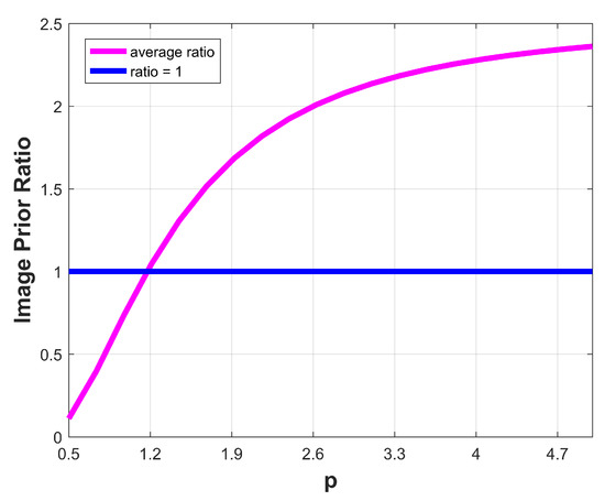
Figure 1.
The statistical evaluation of average prior ratios for different values of p on the dataset [19]. The average prior ratios are always larger than one when . This illustrates that the choice of makes the average energy values of the sharp solutions lower than the blurred ones.
3.2. Optimization
We solve (4) by alternative optimizing on u and k. The optimization details of two sub-problems are described in the following.
3.2.1. Blind Kernel Estimation
Intermediate Image Estimation. With the blur kernel k output from the previous iteration, the intermediate latent image u is estimated by
We use the iterative reweighed least squares (IRLS) [42] method to solve (5). At the t-th iteration, we need to solve the following quadratic problem:
where , , t denotes the iteration index, and the subscript denotes the spatial location of a pixel. (6) is a weighted least squares problem which can be solved by the conjugate gradient method.
Kernel Estimation. Given a fixed intermediate latent image u, the blur kernel k can be obtained by solving the following model
According to the analysis in [9], the kernel estimation methods in gradient domain can be more accurate. Thus, we replace the image intensity with the image derivatives in the data fidelity. That is, the blur kernel k is estimated by
Because of the benefit from the transformed deconvolution formulation (4), we are not required to impose normalization on the blur kernel k practically. Similar to most existing methods, after obtaining k, we set its negative elements to be 0, and divide it by its norm so that the sum of its elements is 1.
To get better results, the proposed kernel estimation process is carried out in a coarse-to-fine manner using an image pyramid. u and k are initialized as the blurred image and delta kernel in the coarsest level.
3.2.2. Final Deblurring
With the blur kernel k being determined, a variety of non-blind deconvolution methods can be used to estimate the latent image. We simply employ a hyper-Laplacian prior proposed by Levin et al. [42] to recover the latent image. The formulation of this non-blind deconvolution method is
Figure 2 illustrates the whole pipeline of our framework. Algorithm 1 presents the main steps for the whole deblurring process. Figure 3 shows the diagram of the proposed algorithm.
| Algorithm 1 Proposed blind deblurring algorithm |
| Input: Blurred image f. Initialize the intermediate image u and kernel k with the results from the coarser level. for do Estimate u according to (5); Estimate k according to (8). end for Estimate the final latent image by solving (10). Output: Latent image u and blur kernel k. |
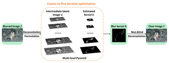
Figure 2.
The pipeline of the proposed algorithm. In this algorithm, u and k are solved iteratively for each image scale in a coarse-to-fine pyramid framework.
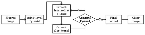
Figure 3.
The pipeline of the proposed algorithm. In this algorithm, u and k are solved iteratively for each image scale in a coarse-to-fine pyramid framework.
4. Discussion and Experimental Results
In this section, we first show some discussions of the proposed method in Section 4.1: we empirically determine an optimal value of p in terms of three evaluation criterions in Section 4.1.1. According to this p, we discuss the convergence property of the proposed algorithm in Section 4.1.2 and provide the parameter analysis in Section 4.1.3. The limitations are discussed in Section 4.1.4. Then we evaluate the proposed method on both synthetic and real-world blurred images and compare it to state-of-the-art image deblurring methods in Section 4.2.
The proposed algorithm is implemented in MATLAB on a computer with an Intel Xeon E5630 CPU G and 12 GB RAM. To process a blurred image with kernel size , the proposed algorithm estimates the blur kernel in around 69 seconds without code optimization.
Parameter settings. In all experiments, the regularization weight parameter is set to be , is set to be , and p is set to be 2.
4.1. Discussion
4.1.1. Determination on Parameter p
In the proposed method, the parameter p plays a critical role as it implicitly influences the normalization of the blur kernel. It is also difficult to be determined theoretically. In order to choose a suitable p, we carried out experiments on a synthetic dataset to test 19 different values of p varying from to 5, the step size for p is . To generate blurred images, we randomly pick 100 images from the BSDS500 dataset [43] and blur them by 8 kernels introduced by [19]. Three commonly used evaluation criterions, kernel similarity, error ratio and PSNR , are utilized for evaluation.
The kernel similarity measures the accuracy of the estimated kernel over ground-truth kernel . This metric calculates the maximum response of normalized cross-correlation between and with some possible shift. The error ratio metric proposed by [19] is commonly used to evaluate the restored result, and the PSNR is commonly used metric to evaluate the quality of the recovered results in comparison with ground-truth images.
The statistical results are summarized in Figure 4. In the subfigures, the three horizontal axes denote the values of p, and the three vertical axes denote the average kernel similarity, average error ratio and average PSNR, respectively. As can be seen in Figure 4a, in terms of the average kernel similarity, the optimal p lies in . Figure 4b demonstrates that when , the proposed method generates results with error ratio values smaller than 2. Other p values have relatively large error ratio values. In Figure 4c, we observe that p values in achieve average PSNR higher than 25, and the highest one is reached when . Based on above observations, we set in all of our experiments.
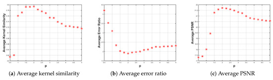
Figure 4.
Evaluation for deblurring methods with different p values on a synthetic dataset which contains 800 images. In terms of the three evaluation criterions, appears to be a good choice.
4.1.2. Convergence Property
We present the convergence property of the proposed method when in this section. For better demonstration, we quantitatively evaluate the convergence property of the proposed method on the benchmark dataset introduced by [19]. The results shown in Figure 5 demonstrate that the proposed method converges after less than 10 iterations, in terms of the average kernel similarity and average energies computed from model (5).
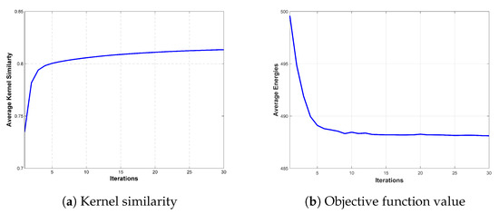
Figure 5.
Convergence property of the proposed algorithm with in terms of two commonly used evaluation criterions.
4.1.3. Parameter Analysis
The proposed model involves two main parameters, and . The parameter is used in the final non-blind deblurring step to recover the final deblurred images with the estimated kernels. For the selection of , we follow the existing non-blind deblurring algorithm [42]. The parameter is a regularization weight parameter. We evaluate the effects of the parameter on deblurred results on the dataset [19] with the average kernel similarity metric and average PSNR value. Figure 6 shows that the selection of does not have very great influences on the quality of the deblurred results. Overall, the proposed algorithm achieves the best performance when . Based on these statistical evaluations, the regularization weight parameter is empirically set to be in all experiments.
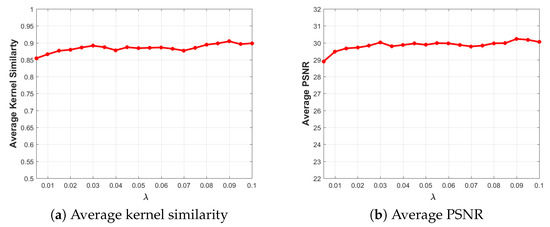
Figure 6.
Effects of varying on the performances of the proposed method.
4.1.4. Limitations
The proposed method is based on an existing simple image prior. It may fail in some cases. Here we present one special case. As our method is under the uniform-blur assumption, if an image is blurred non-uniformly, like rotation blur, our method cannot restore the image effectively. Figure 7a shows one real example. As can be seen in Figure 7b, our method fails to generate desirable results.
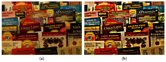
Figure 7.
One failure real example. (a) An image blurred non-uniformly. (b) Our deblurred result of (a). Our method can not deal with non-uniform deblurring.
4.2. Experimental Results
4.2.1. Quantitative Evaluation on Synthetic Datasets
To better evaluate the effectiveness of the proposed method, we perform experiments on three mainstream benchmark datasets [8,19,44]. For fair comparison, we use the implementations of the state-of-the-art methods to estimate the blur kernels. The non-blind deconvolution method [42] is utilized to generate the final deblurring results.
We first test our method on the benchmark dataset [19]. This dataset contains 32 blurred images from 4 ground-truth images with 8 blur kernels. We compare our method with 9 state-of-the-art methods including Levin et al. [11], Krishnan et al. [10], Perrone and Favaro [14], Michaeli and Iran [13], Ren et al. [3], Dong et al. [23], Yan et al. [16], Pan et al. [5] and Jin et al. [17]. We evaluate the effectiveness of the proposed method by both error ratio and average kernel similarity.
Figure 8 shows the comparisons of the cumulative error ratios and average kernel similarity. The graph in Figure 8a shows that when the error ratio is greater than , our success rate exceeds . In comparison, the success rate of Yan et al. [16], which performs the best in the 9 compared methods, reaches to until the error ratio being up to . Similarly, the proposed method has higher average kernel similarity values than other compared methods, as demonstrated in Figure 8b.
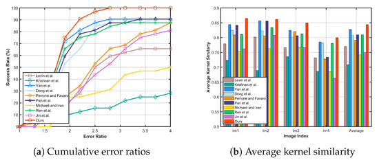
Figure 8.
Quantitative evaluation on the dataset by Levin et al. [19]. Comparisons on these two quality metrics demonstrate that our method performs well against the other methods.
Next, we test our method on the benchmark dataset [44], which contains 4 images and 12 blur kernels. We also show the performances of the proposed method against 7 state-of-the-art methods including Krishnan et al. [10], Shan et al. [20], Perrone and Favaro [14], Ren et al. [3], Pan et al. [5], Dong [23] and Jin et al. [17] in terms of error ratio and average PSNR. As shown in Figure 9a, our method takes lead with of the output under error ratio . Figure 9b shows that our method has the highest average PSNR among all the methods evaluated.
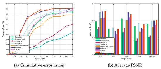
Figure 9.
Quantitative evaluation on the dataset [44]. In particular, our method is up to success rate at error ratio . For average PSNR value, our method achieves on average, leading among state-of-the-art methods.
Moreover, we evaluate our method on the benchmark dataset provided by Lai et al. [8], which contains 100 images including low-illumination, face, and text images. We compare our method with 7 state-of-the-art methods: Perrone and Favaro [14], Michaeli and Iran [13], Pan et al. [5], Ren et al. [3], Dong [23], Yan et al. [16] and Jin et al. [17]. The error ratio and average PSNR are used as performance evaluation criterions on this dataset. Figure 10a presents the cumulatively distribution of error ratios, our method is able to exceed success rate when error ratio is greater than , which performs the best in the 7 compared methods. Figure 10b shows that the proposed method performs well in terms of average PSNR.
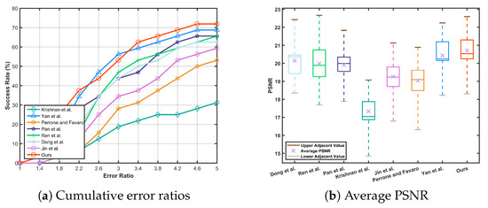
Figure 10.
Quantitative evaluation on the dataset proposed by Lai et al. [8]. Our method exceeds success rate at the error ratio and generates results having the highest average PSNR.
In addition, we test our method on some other synthetic images. To provide visual comparisons, we show two examples in Figure 11. The numbers in green presented on the top left corner in each image are the PSNRs values, which quantitatively measure the quality of the deblurring methods. Both visually and quantitatively, Figure 11 shows that the proposed method achieves favorable results against the other deblurring methods.
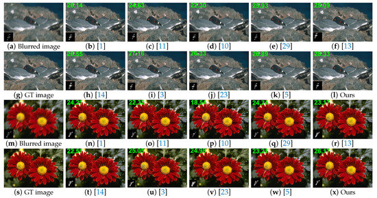
Figure 11.
Visual comparisons on two synthetic examples from the BSDS500 dataset [43]. Results are deblurred by Xu and Jia [1], Levin et al. [11], Krishnan et al. [10], Sun et al. [29], Michaeli and Iran [13], Perrone and Favaro [14], Ren et al. [3], Dong et al. [23] and Pan et al. [5], respectively.
4.2.2. Deblurring on Real Blurred Images
We note that the existing two methods [10,14] have very similar formulation to (4). So we first show an example in Figure 12 compared with these two methods. The deblurring results shown in Figure 12b,c still contain severe blur effects and ringing artifacts. In comparison, our result shown in Figure 12d is better.
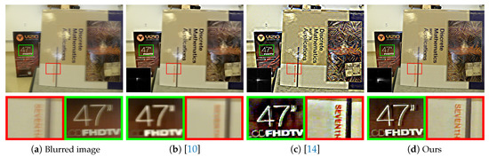
Figure 12.
Visual comparisons on a real blurred image. (a) Blurred image. (b) Krishnan et al. [10]. (c) Perrone and Favaro [14]. (d) Ours. The recovered image by our method is visually clearer than others.
Figure 13 shows another real blurred example compared with the state-of-the-art deblurring methods [1,5,10,13,14,15,17,29]. The close-ups of the deblurred results by [10,15], which are shown in Figure 13c,h, contain significant blur, especially in the text region. The deblurred results by the methods [13,29] contain significant ringing artifacts, as shown in Figure 13d,e. The deblurred result by Jin et al. [17], which is shown in Figure 13k, contains some unpleasing effects. Although the method [1,3,5,14,23] handle this image well, their deblured results contain some noises around the text in the background as shown in Figure 13b,f,g,i,j, respectively. In contrast, our method generates clear result with less noise. The text and background of the deblurred result by our method are much clearer than other methods.
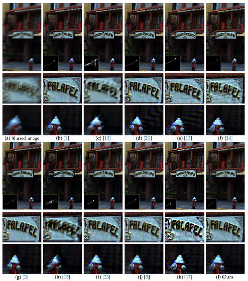
Figure 13.
Comparisons on a real blurred image. (a) Blurred image. (b) Xu and Jia [1]. (c) Krishnan et al. [10]. (d) Sun et al. [29]. (e) Michaeli and Iran [13]. (f) Perrone and Favaro [14]. (g) Ren et al. [3]. (h) Pan et al. [15]. (i) Dong et al. [23]. (j) Pan et al. [5]. (k) Jin et al. [17]. (l) Ours. Compared with other results, our deblurred result is more pleasing.
Another one real blurred image is shown in Figure 14a. The results by methods [10,23,27], shown in Figure 14b,g,i, contain some blur effects. In Figure 14c,d,e,h, the results by methods [13,14,17,29] contain significant ringing artifacts. The result by [3] is visually better than the above results as shown in Figure 14f. Compared with it, our method generates the deblurred image with clearer details as shown in Figure 14j.
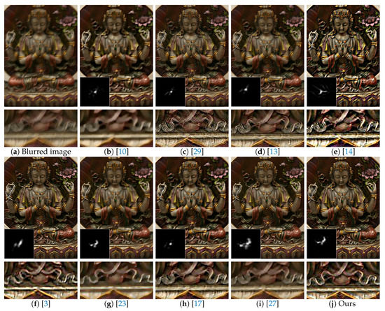
Figure 14.
Comparisons on a real blurred image. (a) Blurred image. (b) Krishnan et al. [10]. (c) Sun et al. [29]. (d) Michaeli and Iran [13]. (e) Perrone and Favaro [14]. (f) Ren et al. [3]. (g) Dong et al. [23]. (h) Jin et al. [17]. (i) Li et al. [27]. (j) Ours. Compared with the state-of-the-art deblurring methods, our method generates a clear image with fine details.
Figure 15 shows one example from the dataset [44] compared with [1,3,10,11,13,14,15,23]. The deblurring methods [1,13,23] produce ringing artifacts as shown in Figure 15b,e,h. The deblurring results by methods [3,11,15] are over smoothed as shown in Figure 15c,g,i. The deblurred result by Krishnan et al. [10] in Figure 15d still contains some noise. The deblurred result by Perrone and Favaro [14], which is shown in Figure 15f, is also unpleasing. In contrast, our method generates a much clearer result, as shown in Figure 15j.
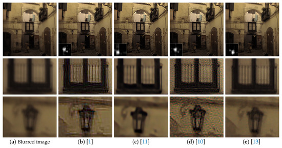
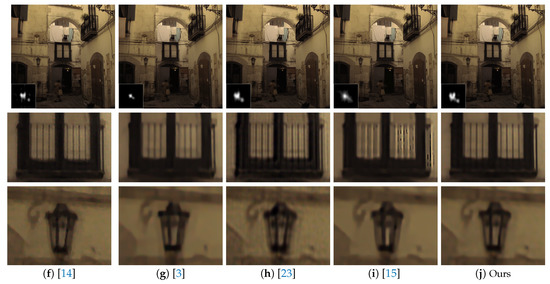
Figure 15.
Comparisons of deblurred results with close-ups of an example from the dataset [44]. (a) Blurred image. (b) Xu and Jia [1]. (c) Levin et al. [11]. (d) Krishnan et al. [10]. (e) Michaeli and Iran [13]. (f) Perrone and Favaro [14]. (g) Ren et al. [3]. (h) Dong et al. [23]. (i) Pan et al. [15]. (j) Ours. The recovered image by the proposed algorithm is visually more pleasing.
In addition, we provide visual comparisons with the state-of-the-art deep learning based methods in Figure 16. The deep learning based methods [35,37] are less effective in handling this blurred image as shown in Figure 16b,c. The result by the method [27] in Figure 16d is visually acceptable. In comparison, our result shown in Figure 16e is clearer than their result as shown in Figure 16d.
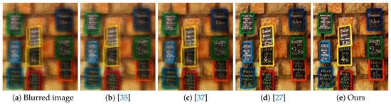
Figure 16.
Visual comparisons on a real wold blurred image with the state-of-the-art deep learning based methods. (a) Blurred image. (b) Kupyn et al. [35]. (c) Tao et al. [37]. (d) Li et al. [27]. (e) Ours. Our method performs favorably against the state-of-the-art deep learning methods.
4.2.3. Domain Specific Images
We further evaluate our method on two kinds of domain specific images, e.g., text and face images. Text images are rather challenging for most deblurring methods. Figure 17 displays the deblurring results on two text images. For fair comparison, the final deblurred results of both kernel prior based methods and our method are recovered by the non-blind deblurring method [42]. Figure 17b shows the results by employing kernel prior (). Figure 17c shows the results by using kernel prior () and Figure 17d shows the results by the text deblurring method [15]. Comparing to the deblurred results using kernel prior for the logo text image, our method estimates the kernel structure correctly while the other methods fail as shown in the top row of Figure 17. The bottom row of Figure 17 shows the deblurring results for a document text image. We note that our method generates better result than using kernel prior and we obtain a comparable result with the specially designed text deblurring method [15].
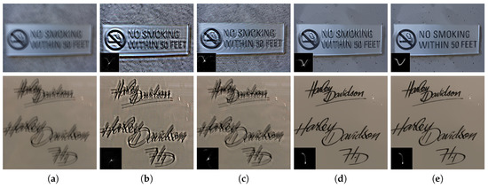
Figure 17.
Comparisons on two text blurred images. (a) Blurred image. Results shown in (b–e) are deblurred by kernel prior, kernel prior, Pan et al. [15] and ours, respectively. Our method generates better results than the previous two kernel prior methods and we obtain visually comparable or even better results than the specially designed for text deblurring method [15].
Face images deblurring is challenging due to the blurry face images contain few edges or textures. Figure 18 shows some deblurring results on a face image. As can be seen, there are several artifacts in most of the results deblurred by other state-of-the-art methods, as shown in Figure 18b–k. Our method generates a clearer result with less ringing artifacts as shown in Figure 18l.
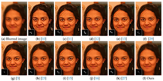
Figure 18.
Deblurred results on a face image. (a) Blurred image. (b) Krishnan et al. [10]. (c) Levin et al. [11]. (d) Xu et al. [12]. (e) Michaeli and Iran [13]. (f) Sun et al. [29]. (g) Ren et al. [3]. (h) Dong et al. [23]. (i) Pan et al. [15]. (j) Yan et al. [16]. (k) Li et al. [27]. (l) Ours. Our method generates visually more pleasing result with fewer ringing artifacts.
5. Conclusions and Future Work
In this paper, we consider the relative scale ambiguity between the latent image and the blur kernel based on an existing hyper-Laplacian regularization. We impose normalization constraint on the blur kernel instead of the arbitrary normalization constraint, which has been selected in most existing deblurring methods. We present that the hyper-Laplacian regularization can be transformed to a joint prior. Statistical results demonstrate that the joint prior favors ground-truth sharp solutions over trivial solutions when , which facilitates our deconvolution formulation to avoid trivial solutions. To determine the parameter p, we carry out numerical experiments and find that can be a good choice. Both quantitative and qualitative experiments on benchmark datasets and real images demonstrate that the proposed method is able to achieve the state-of-the-art results without any heuristic filtering strategies to select salient edges or kernel sparsity prior. Our future work will focus on focus on considering the scale ambiguity by imposing the normalization constraint on the blur kernel associated with other image priors and improving the computational efficiency to implement realtime processing on the embedded platform.
Author Contributions
Conceptualization, W.F. and H.W.; methodology, W.F. and H.W.; software, W.F.; validation, W.F. and Y.W.; formal analysis, W.F. and H.W.; investigation, W.F.; data curation, W.F.; writing—original draft preparation, W.F.; writing—review and editing, H.W. and W.F.; visualization, W.F.; supervision, Z.S.; project administration, Z.S.; funding acquisition, Z.S. All authors have read and agreed to the published version of the manuscript.
Funding
This work has been partially supported by National Natural Science Foundation of China under Grant 61976041.
Conflicts of Interest
The authors declare no conflict of interest.
References
- Xu, L.; Jia, J. Two-Phase Kernel Estimation for Robust Motion Deblurring. ECCV 2010, 157–170. [Google Scholar] [CrossRef]
- Perrone, D.; Favaro, P. A Logarithmic Image Prior for Blind Deconvolution. Int. J. Comput. Vis. 2016, 117, 159–172. [Google Scholar] [CrossRef]
- Ren, W.; Cao, X.; Pan, J.; Guo, X.; Zuo, W.; Yang, M.H. Image Deblurring via Enhanced Low Rank Prior. IEEE Trans. Image Process. 2016, 25, 3426–3437. [Google Scholar] [CrossRef] [PubMed]
- Pan, J.; Dong, J.; Tai, Y.; Su, Z.; Yang, M. Learning Discriminative Data Fitting Functions for Blind Image Deblurring. ICCV 2017, 1077–1085. [Google Scholar] [CrossRef]
- Pan, J.; Sun, D.; Pfister, H.; Yang, M. Deblurring Images via Dark Channel Prior. IEEE Trans. Pattern Anal. Mach. Intell. 2018, 40, 2315–2328. [Google Scholar] [CrossRef]
- Pan, J.; Ren, W.; Hu, Z.; Yang, M. Learning to Deblur Images with Exemplars. IEEE Trans. Pattern Anal. Mach. Intell. 2019, 41, 1412–1425. [Google Scholar] [CrossRef]
- Zheng, H.; Ren, L.; Ke, L.; Qin, X.; Zhang, M. Single image fast deblurring algorithm based on hyper-Laplacian model. IET Image Process. 2019, 13, 483–490. [Google Scholar] [CrossRef]
- Lai, W.; Huang, J.; Hu, Z.; Ahuja, N.; Yang, M. A Comparative Study for Single Image Blind Deblurring. CVPR 2016, 1701–1709. [Google Scholar] [CrossRef]
- Cho, S.; Lee, S. Fast motion deblurring. ACM Trans. Graph. 2009, 28, 145. [Google Scholar] [CrossRef]
- Krishnan, D.; Tay, T.; Fergus, R. Blind deconvolution using a normalized sparsity measure. CVPR 2011, 233–240. [Google Scholar] [CrossRef]
- Levin, A.; Weiss, Y.; Durand, F.; Freeman, W.T. Efficient marginal likelihood optimization in blind deconvolution. CVPR 2011, 2657–2664. [Google Scholar] [CrossRef]
- Xu, L.; Zheng, S.; Jia, J. Unnatural L0 Sparse Representation for Natural Image Deblurring. CVPR 2013, 1107–1114. [Google Scholar] [CrossRef]
- Michaeli, T.; Irani, M. Blind Deblurring Using Internal Patch Recurrence. ECCV 2014, 783–798. [Google Scholar] [CrossRef]
- Perrone, D.; Favaro, P. Total Variation Blind Deconvolution: The Devil Is in the Details. CVPR 2014, 2909–2916. [Google Scholar] [CrossRef]
- Pan, J.; Hu, Z.; Su, Z.; Yang, M. L0-Regularized Intensity and Gradient Prior for Deblurring Text Images and Beyond. IEEE Trans. Pattern Anal. Mach. Intell. 2017, 39, 342–355. [Google Scholar] [CrossRef]
- Yan, Y.; Ren, W.; Guo, Y.; Wang, R.; Cao, X. Image Deblurring via Extreme Channels Prior. CVPR 2017, 6978–6986. [Google Scholar] [CrossRef]
- Jin, M.; Roth, S.; Favaro, P. Normalized Blind Deconvolution. ECCV 2018, 694–711. [Google Scholar] [CrossRef]
- Wen, G.; Min, C.; Jiang, Z.; Yang, Z.; Li, X. Patch-Wise Blind Image Deblurring Via Michelson Channel Prior. IEEE Access 2019, 7, 181061–181071. [Google Scholar] [CrossRef]
- Levin, A.; Weiss, Y.; Durand, F.; Freeman, W.T. Understanding and evaluating blind deconvolution algorithms. CVPR 2009, 1964–1971. [Google Scholar] [CrossRef]
- Shan, Q.; Jia, J.; Agarwala, A. High-quality motion deblurring from a single image. ACM Trans. Graph. 2008, 27, 73. [Google Scholar] [CrossRef]
- Zhang, Y.; Lau, Y.; Kuo, H.; Cheung, S.; Pasupathy, A.; Wright, J. On the Global Geometry of Sphere-Constrained Sparse Blind Deconvolution. CVPR 2017, 4381–4389. [Google Scholar] [CrossRef]
- Srivastava, A.; Lee, A.B.; Simoncelli, E.P.; Zhu, S. On Advances in Statistical Modeling of Natural Images. J. Math. Imaging Vis. 2003, 18, 17–33. [Google Scholar] [CrossRef]
- Dong, J.; Pan, J.; Su, Z. Blur kernel estimation via salient edges and low rank prior for blind image deblurring. Signal Process. Image Commun. 2017, 58, 134–145. [Google Scholar] [CrossRef]
- Dong, J.; Pan, J.; Sun, D.; Su, Z.; Yang, M. Learning Data Terms for Non-blind Deblurring. ECCV 2018, 777–792. [Google Scholar] [CrossRef]
- Jiang, X.; Yao, H.; Zhao, S. Text image deblurring via two-tone prior. Neurocomputing 2017, 242, 1–14. [Google Scholar] [CrossRef]
- Tang, Y.; Xue, Y.; Chen, Y.; Zhou, L. Blind deblurring with sparse representation via external patch priors. Digit. Signal Process. 2018, 78, 322–331. [Google Scholar] [CrossRef]
- Li, L.; Pan, J.; Lai, W.; Gao, C.; Sang, N.; Yang, M.H. Blind Image Deblurring via Deep Discriminative Priors. Int. J. Comput. Vis. 2019, 1–19. [Google Scholar] [CrossRef]
- Chen, L.; Fang, F.; Wang, T.; Zhang, G. Blind Image Deblurring With Local Maximum Gradient Prior. CVPR 2019, 1742–1750. [Google Scholar] [CrossRef]
- Sun, L.; Cho, S.; Wang, J.; Hays, J. Edge-based blur kernel estimation using patch priors. ICCP 2013, 1–8. [Google Scholar] [CrossRef]
- Chang, C.; Wu, J.; Chen, K. A Hybrid Motion Deblurring Strategy Using Patch Based Edge Restoration and Bilateral Filter. J. Math. Imaging Vis. 2018, 60, 1081–1094. [Google Scholar] [CrossRef]
- Chakrabarti, A. A Neural Approach to Blind Motion Deblurring. ECCV 2016, 221–235. [Google Scholar] [CrossRef]
- Yang, C.; Shao, W.; Huang, L. Boosting normalized sparsity regularization for blind image deconvolution. Signal Image Video Process. 2017, 11, 681–688. [Google Scholar] [CrossRef]
- Javaran, T.A.; Hassanpour, H.; Abolghasemi, V. Blind motion image deblurring using an effective blur kernel prior. Multimed. Tools Appl. 2019, 78, 22555–22574. [Google Scholar] [CrossRef]
- Nah, S.; Kim, T.H.; Lee, K.M. Deep Multi-scale Convolutional Neural Network for Dynamic Scene Deblurring. CVPR 2017, 257–265. [Google Scholar] [CrossRef]
- Kupyn, O.; Budzan, V.; Mykhailych, M.; Mishkin, D.; Matas, J. DeblurGAN: Blind Motion Deblurring Using Conditional Adversarial Networks. CVPR 2018, 8183–8192. [Google Scholar] [CrossRef]
- Wang, F.; Liu, H.; Cheng, J. Visualizing deep neural network by alternately image blurring and deblurring. Neural Netw. 2018, 97, 162–172. [Google Scholar] [CrossRef]
- Tao, X.; Gao, H.; Shen, X.; Wang, J.; Jia, J. Scale-Recurrent Network for Deep Image Deblurring. CVPR 2018, 8174–8182. [Google Scholar] [CrossRef]
- Chrysos, G.G.; Favaro, P.; Zafeiriou, S. Motion Deblurring of Faces. Int. J. Comput. Vis. 2019, 127, 801–823. [Google Scholar] [CrossRef]
- Shao, W.; Liu, Y.; Ye, L.; Wang, L.; Ge, Q.; Bao, B.; Li, H. DeblurGAN+: Revisiting blind motion deblurring using conditional adversarial networks. Signal Process. 2020, 168. [Google Scholar] [CrossRef]
- Shi, X.; Chen, Z.; Wang, H.; Yeung, D.; Wong, W.; Woo, W. Convolutional LSTM Network: A Machine Learning Approach for Precipitation Nowcasting. arXiv 2015, arXiv:1506.04214. [Google Scholar]
- Krishnan, D.; Fergus, R. Fast Image Deconvolution using Hyper-Laplacian Priors. NIPS 2009, 1033–1041. [Google Scholar] [CrossRef]
- Levin, A.; Fergus, R.; Durand, F.; Freeman, W.T. Image and depth from a conventional camera with a coded aperture. ACM Trans. Graph. 2007, 26, 70. [Google Scholar] [CrossRef]
- Arbelaez, P.; Maire, M.; Fowlkes, C.C.; Malik, J. Contour Detection and Hierarchical Image Segmentation. IEEE Trans. Pattern Anal. Mach. Intell. 2011, 33, 898–916. [Google Scholar] [CrossRef] [PubMed]
- Köhler, R.; Hirsch, M.; Mohler, B.J.; Schölkopf, B.; Harmeling, S. Recording and Playback of Camera Shake: Benchmarking Blind Deconvolution with a Real-World Database. ECCV 2012, 27–40. [Google Scholar] [CrossRef]


© 2020 by the authors. Licensee MDPI, Basel, Switzerland. This article is an open access article distributed under the terms and conditions of the Creative Commons Attribution (CC BY) license (http://creativecommons.org/licenses/by/4.0/).