Numerical Investigation of Erosion Wear in the Hydraulic Amplifier of the Deflector Jet Servo Valve

Abstract

Although possessing a remarkable anti-contamination capacity, the deflector jet valve is still confronted with erosion wear brought by solid particles in hydraulic oil. To describe the erosion wear mechanism in the hydraulic amplifier of servo valves, a RANS-based CFD simulation is conducted to obtain its internal wear distribution following the Oka erosion model, which shows the erosion wear in servo valves can be divided into four levels and the major wear happens on the shunt wedge, characterized by a regular and fluctuant distribution. Further, there exist multiple relative maximums of erosion rates, whose locations deviate from the jet center. On this basis, the correlation between the contamination level of hydraulic oil and the degree of erosion wear is established. Moreover, according to the working mechanism of the hydraulic amplifier, a new failure criterion of the deflector jet valve is proposed to carry out valve lifespan analyses. Then, a lifespan prediction formula is obtained, and calculations show that hydraulic oil must have a contamination level superior to NAS 5 if a lifespan of over 20,000 h is expected.

1. Introduction

As a promising crucial element in hydraulic transmission equipment, the deflector jet servo valve (DJV) possesses advantages of both extraordinary anti-contamination capacity and great response performance. However, the DJV must be confronted with high-speed jets and intense impacts of fluid on wall materials, bringing about significant erosion wear and issues of the service lifespan. Yet existing research on this topic is so insufficient that it is difficult to estimate the durability and choose an appropriate working condition for valves.

In respect of erosion wear, early research efforts focused on experimental methods and discussions of corresponding results in view of the diversity of erosion conditions and the irregularity of experimental results. Remarkably, erosion experiments with different angles of impact were conducted in the mid-20th century [1,2,3,4], which first confirmed the practical experience by showing variable wear characteristics of different materials with the impact angle changing. In practice erosion wear depends on many factors, such as particle quantity, impact velocity and direction relative to the target surface, as summarized by Finnie [5]. Hence, he came up with a semi-empirical erosion model, the Finnie model, to predict the erosion numerically. Since then more complex erosion models have been presented, including the Tabakoff model [6], the Tulsa model [7], et al. So far one of the most comprehensive models was established by Oka et al. [8,9], in which specific conditions involving impact direction, impact velocity, size of particles, and properties of particles and target material were considered. These erosion models have provided the foundation of numerical investigation and wear prediction in engineering. Then, we have opportunities to explore the erosion wear in valves efficiently, which has been valued in recent years. As a relatively simple scenario, the erosion wear in choke valves was researched based on experimental data of erosion [10]. The relevant erosion equations built by fitting the data were used to obtain the erosion distribution in a CFD-based simulation. Further, on the basis of Harsha’s angle function, a case of the check valve was discussed in detail [11], giving the erosion rates at different flow velocities, particle sizes, valve openings and particle mass rates. However, these valves functioned by fluid throttling rather than jets. While jets in valves mean intense impacts, leading to severe erosion wear. Research on a cylinder blocking the jet has been performed, and the erosion caused by fluid impact was evaluated [12], which unveiled that the central region of the impact was not the most worn location, conforming to the impact angle dependence of erosion wear as already mentioned by Finne [5]. Another investigation of impact erosion came from Zhao [13], who conducted CFD-based simulations and experiments to discuss the erosion distribution on the target plate, with the conclusion that the farther away from the jet center, the greater the wear is. In addition, some research on the erosion wear of jet pipe valves has arisen since 2015. Erosion rate distributions were obtained based on the Edwards model [14,15] and the lifespan was estimated [16], reaching up to 95,000 h. Compared with jet pipe valves, although the DJV has a similar working mechanism, the actual size and working conditions are materially different. Still based on the Edwards model, a description of DJV erosion rate distribution was given to explore the correlation between erosion and the valve performance [17]. However, the simulation showed that maximum erosion happened in the central region of the jet, not consistent with the conclusions of Boulanger [12] and Zhao [13].

Summarizing, although lots of fundamental theories of erosion wear have been provided, the research on the DJV erosion is quite scarce, which cannot bring us a credible and detailed description of erosion distribution. Moreover, the effect of working conditions, such as the contamination level of oil, on erosion wear of the DJV is still indecisive. And without an effective evaluating criterion, there is a research gap about the durability estimation of DJVs. Aiming at this issue, a three-dimensional CFD model is developed to investigate the erosion wear in the pilot hydraulic amplifier of the DJV. Based on the RANS simulation methodology and the Oka erosion model, the erosion distribution in the hydraulic amplifier is obtained to analyze the wear pattern caused by jet impact in DJVs. Then the contamination level dependence of DJV erosion is evaluated, and eventually the lifespan of the valve is predicted in various conditions according to a proposed failure criterion.

The major contributions of the paper are summarized as follows.

(1)

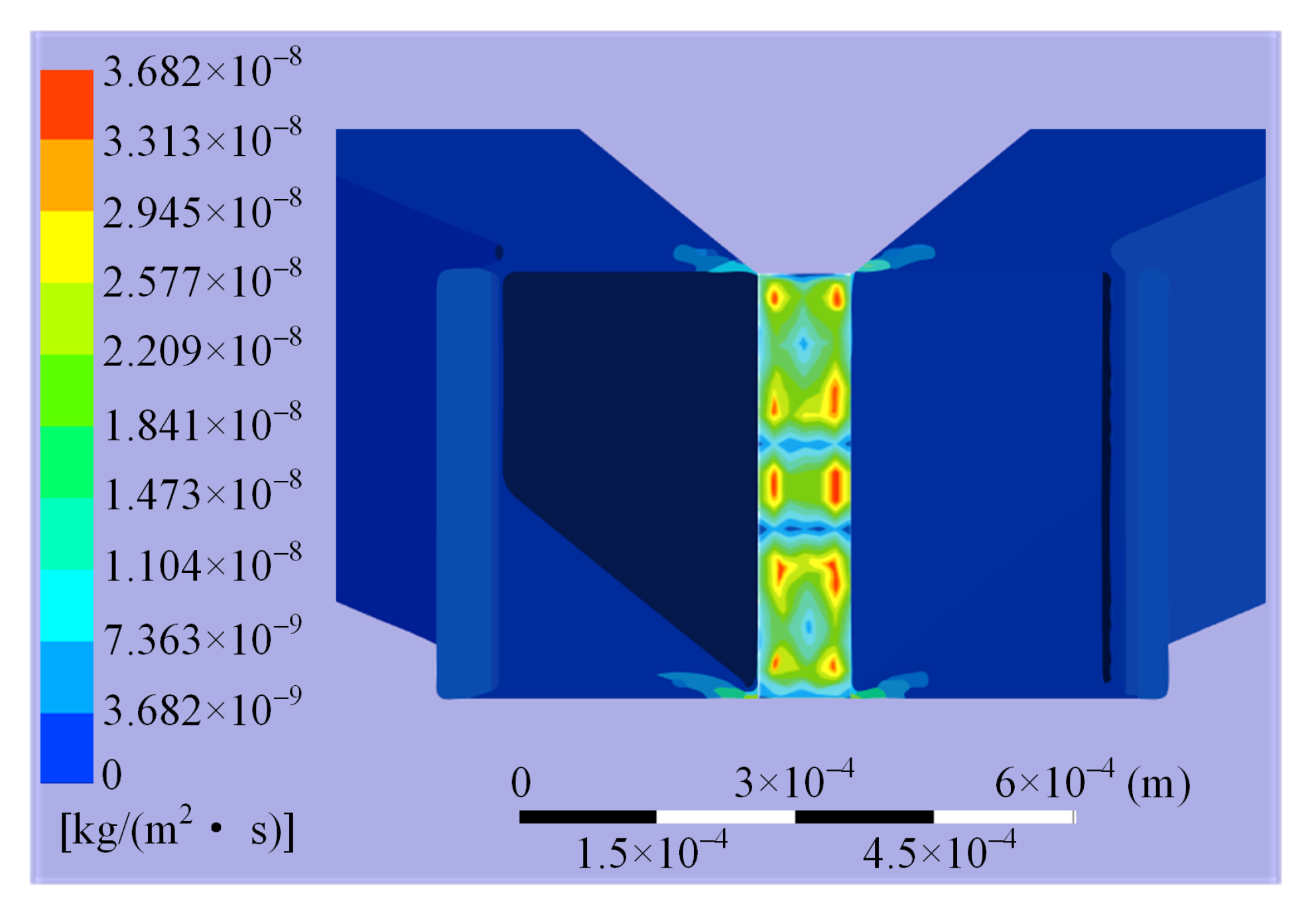
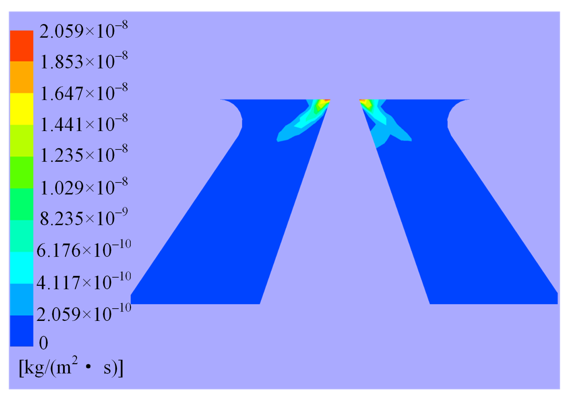
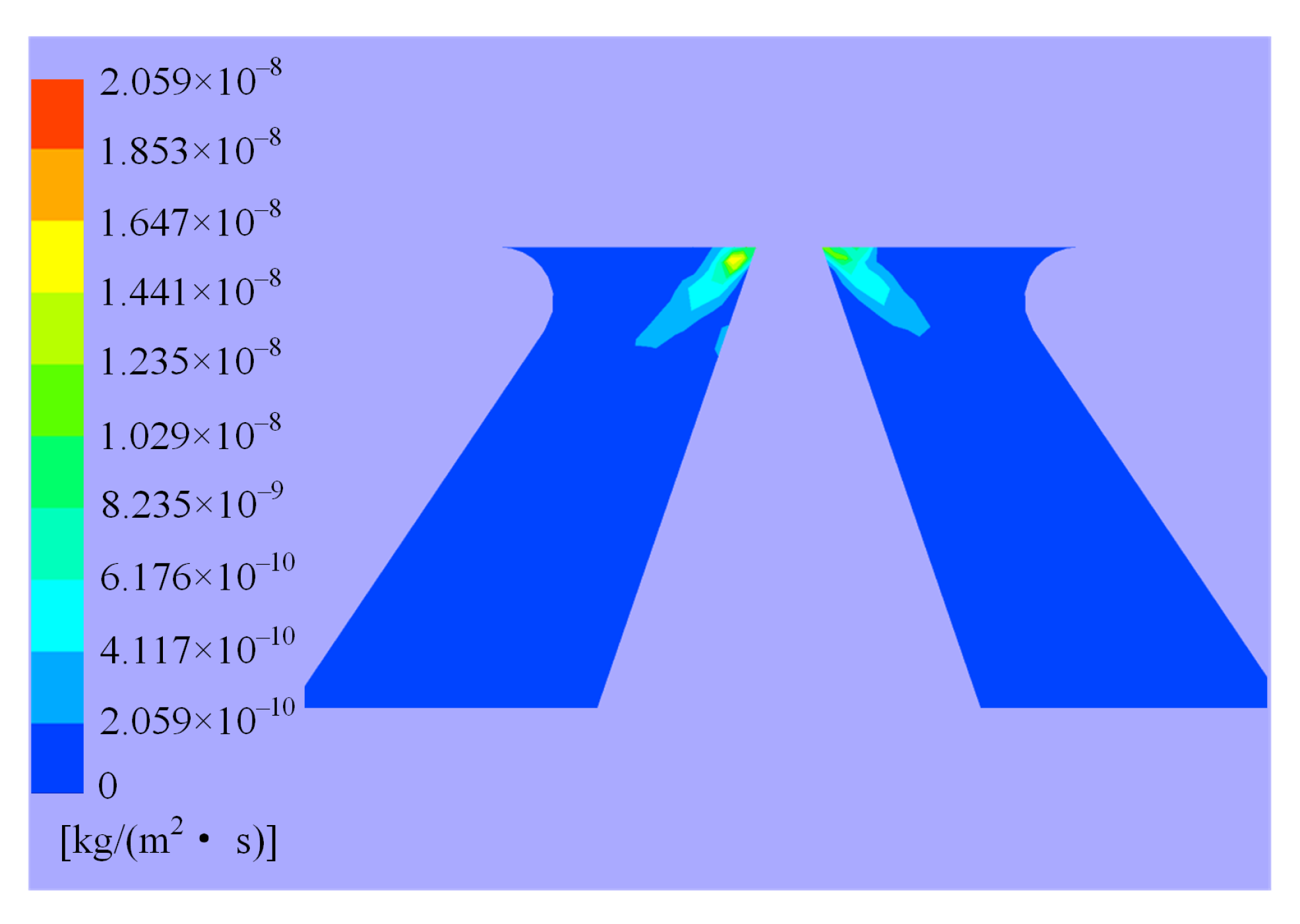
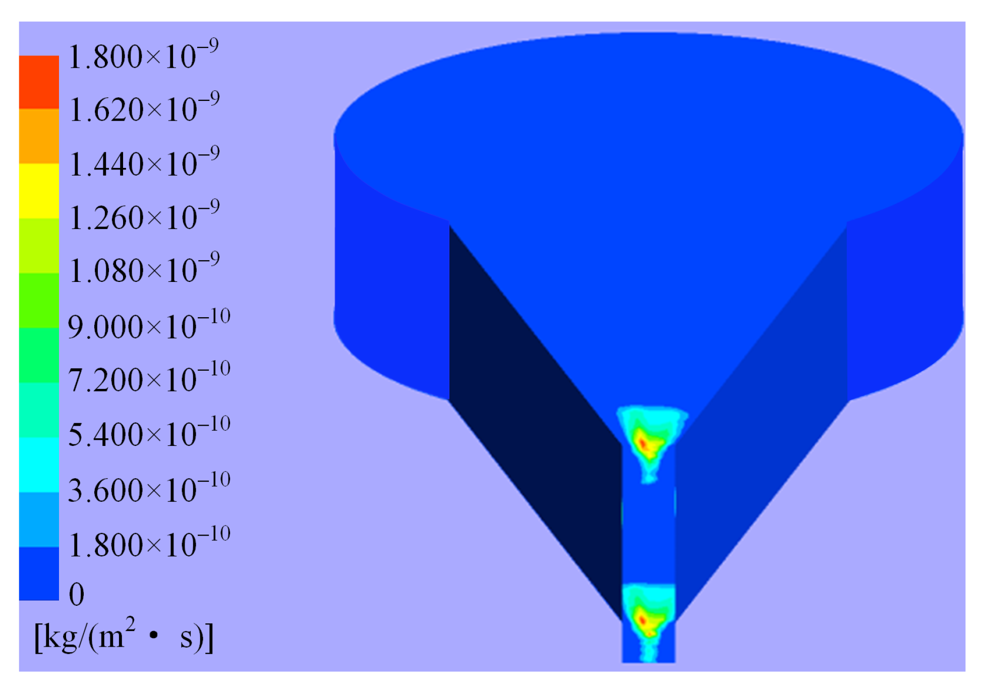
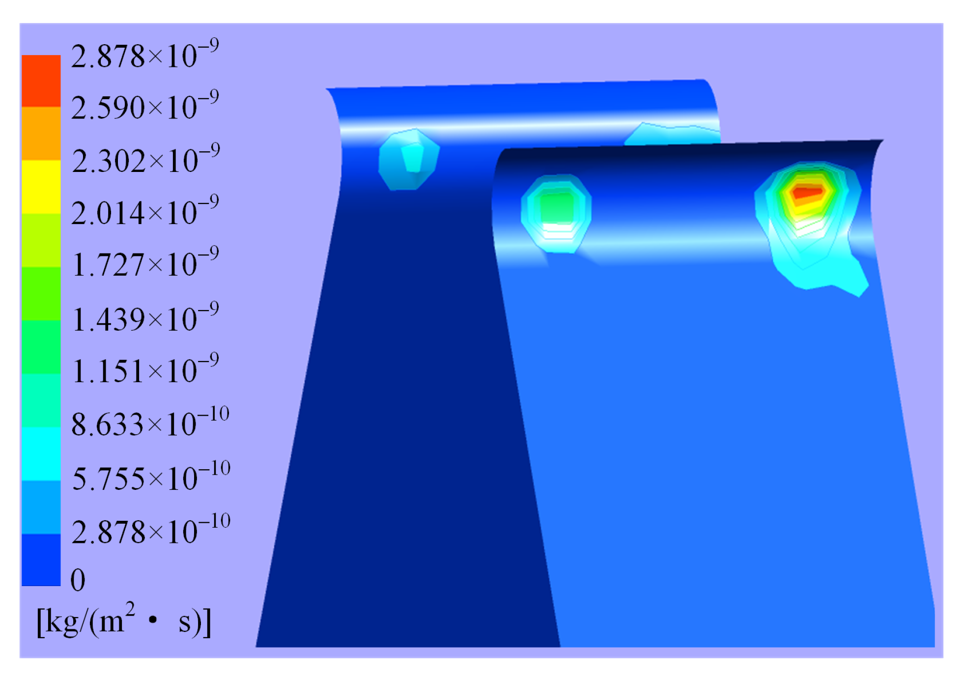
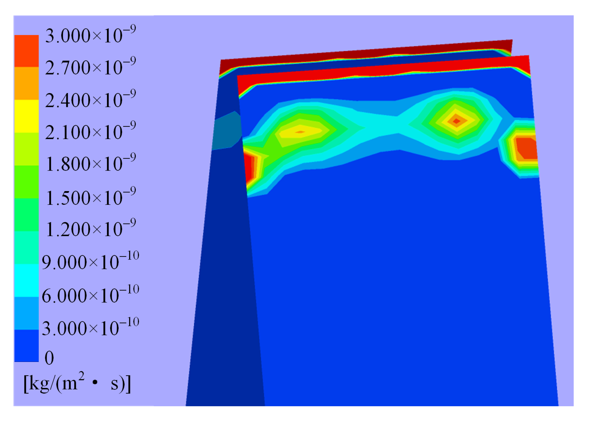
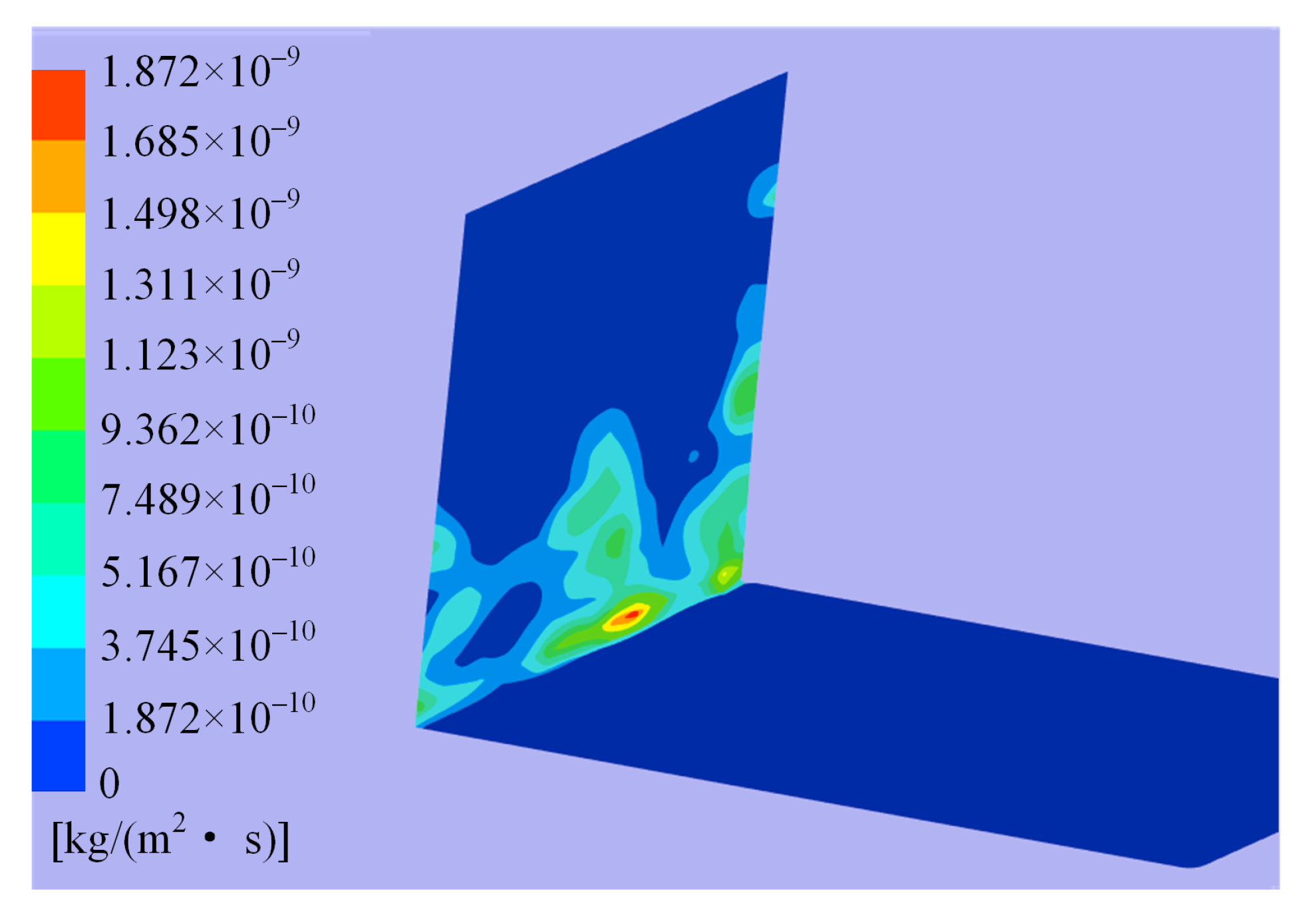
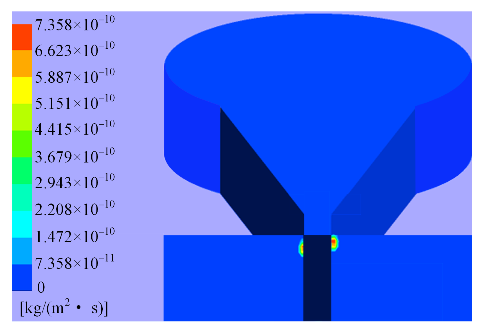
It is found that the erosion wear in the hydraulic amplifier can be divided into four levels according to the order of magnitude of erosion rates, and the major erosion is determined to happen on the shunt wedge.

(2)

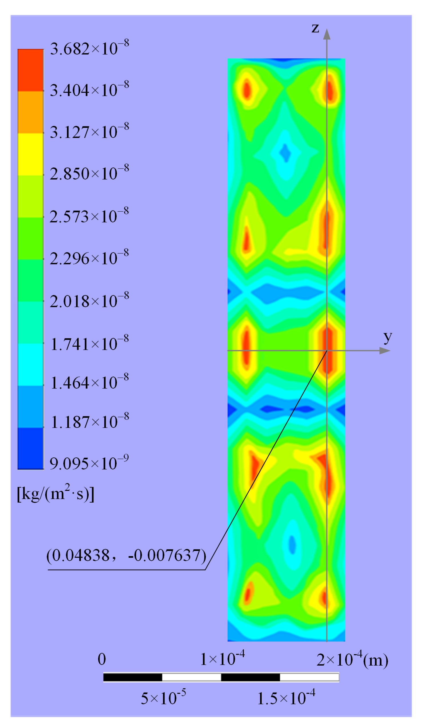
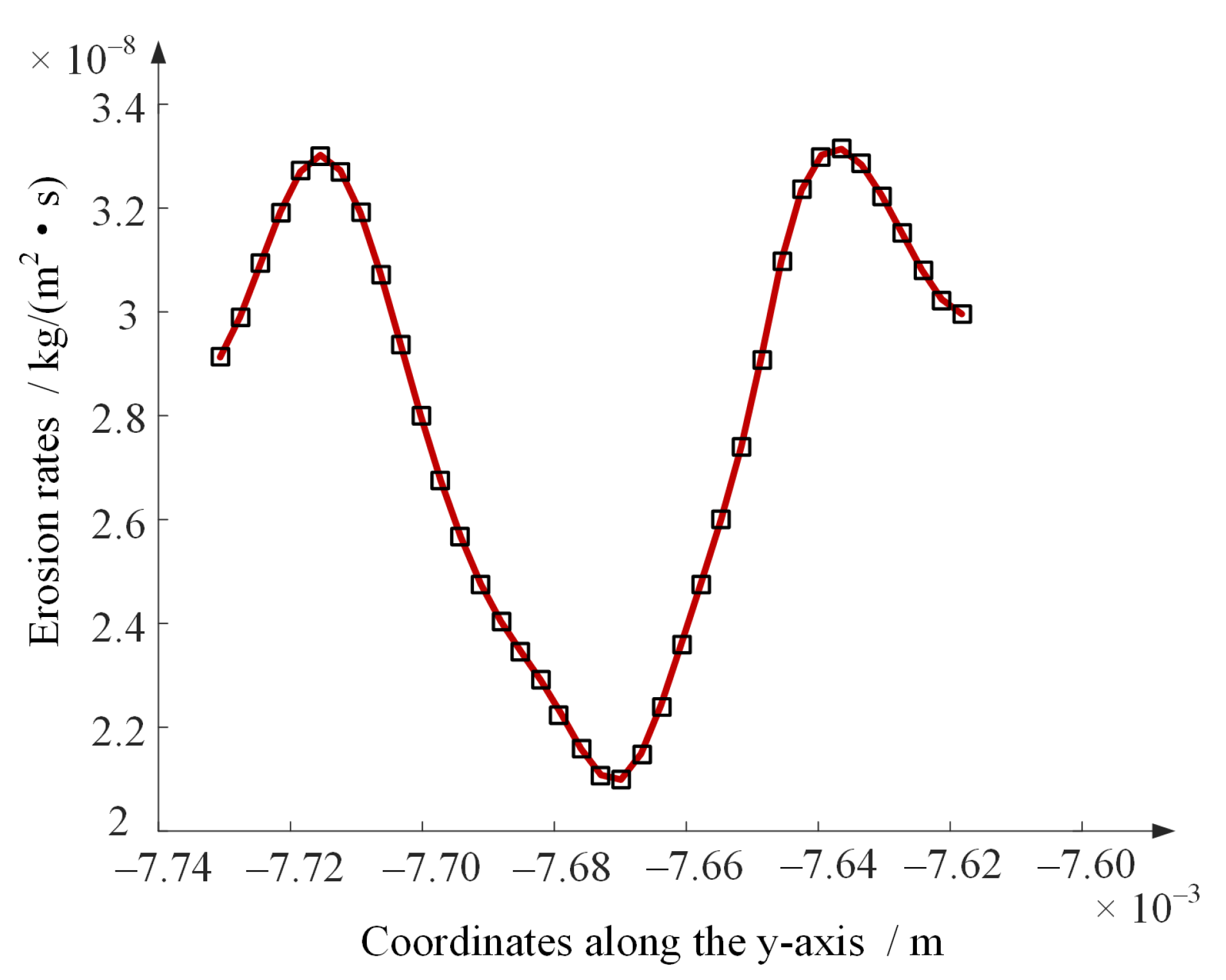
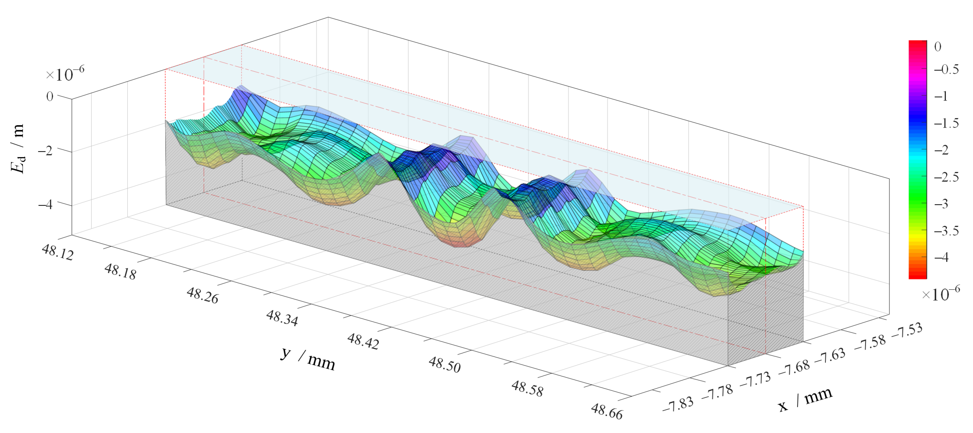
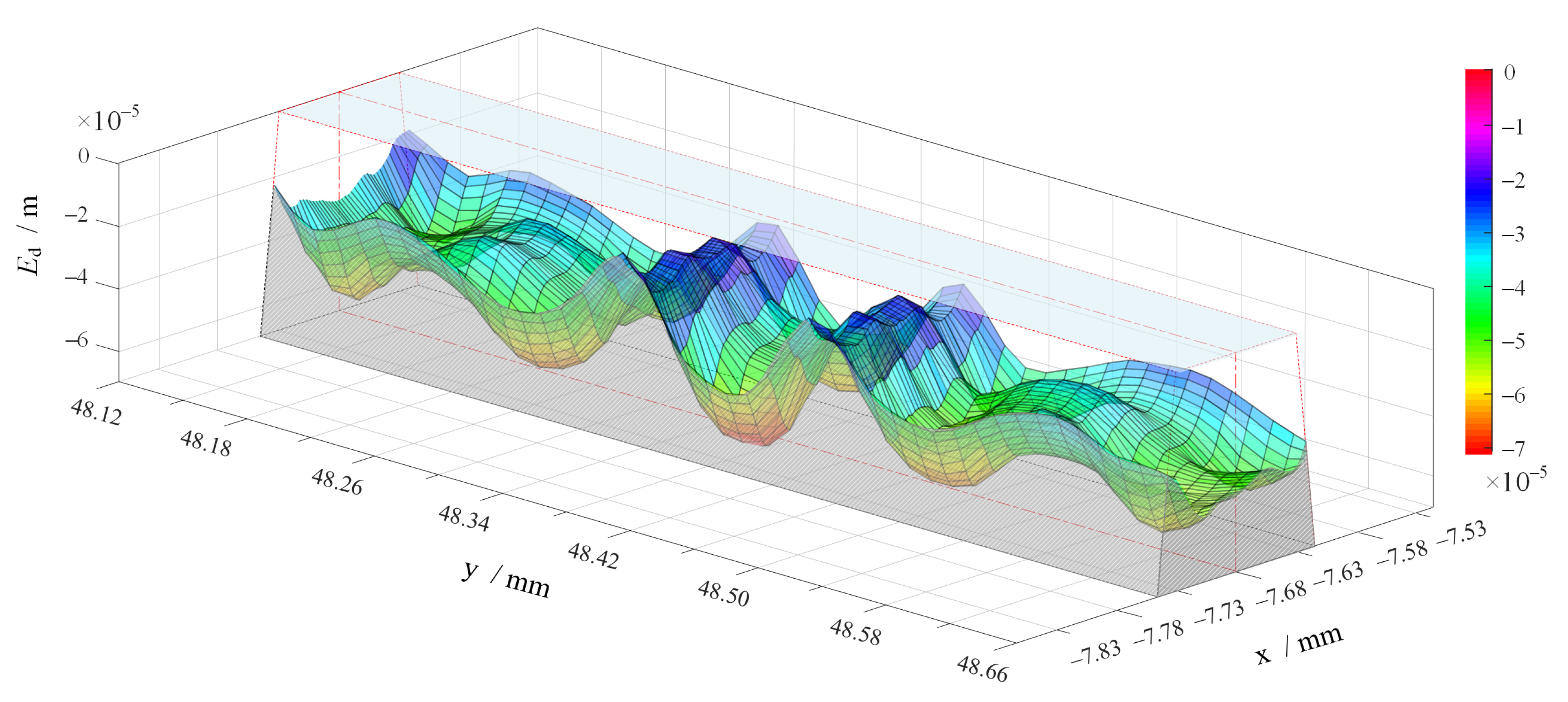
It is observed that the erosion distribution on the shunt wedge caused by jet impact is characterized by regular fluctuations, and there exist multiple relative maximums of erosion rates occurring at places deviating from the jet center.

(3)

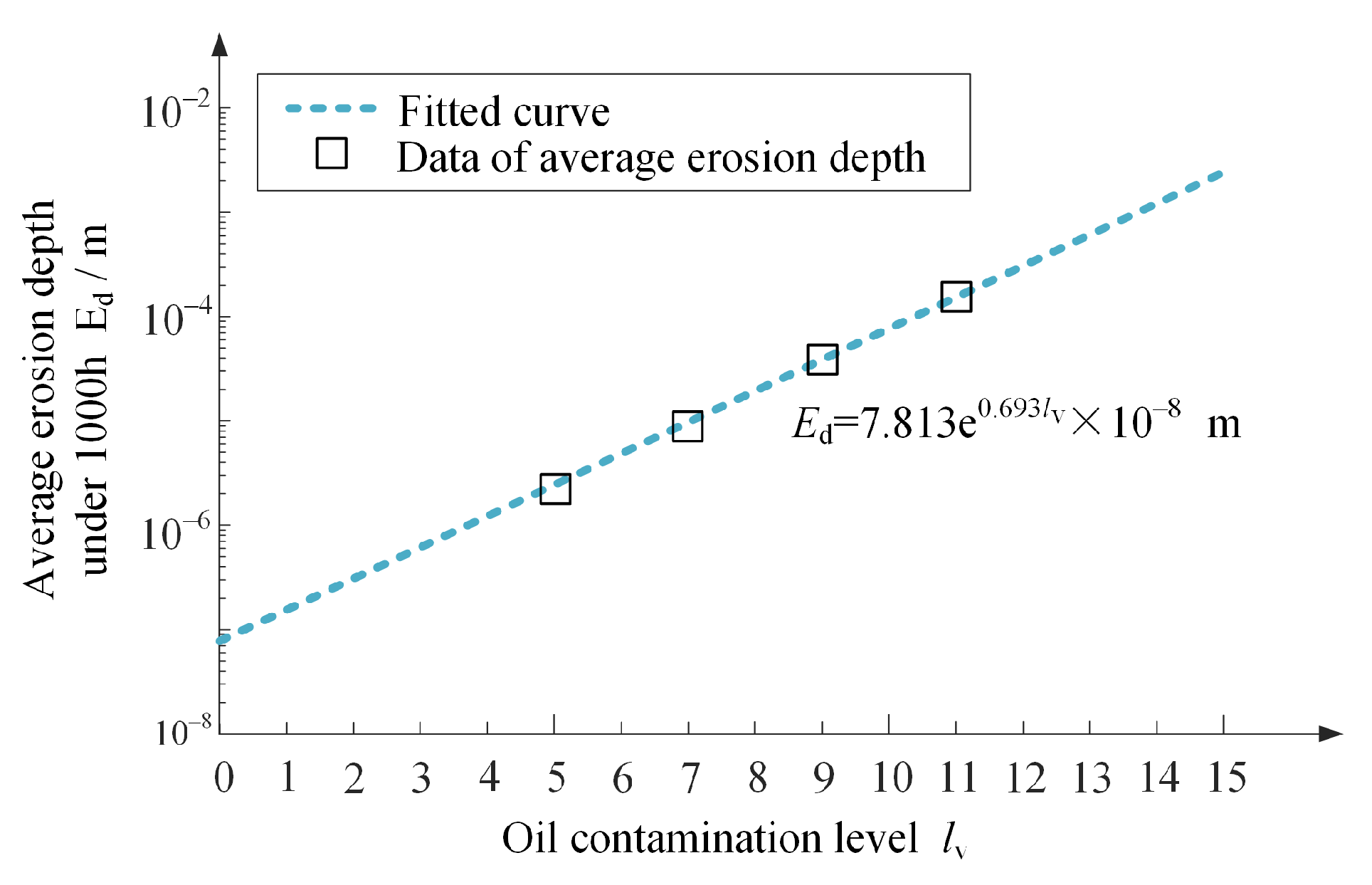
The correlation between the contamination level of hydraulic oil and the extent of erosion wear is depicted and formulated mathematically, giving an intuitive means for understanding the erosion wear in DJVs.

(4)

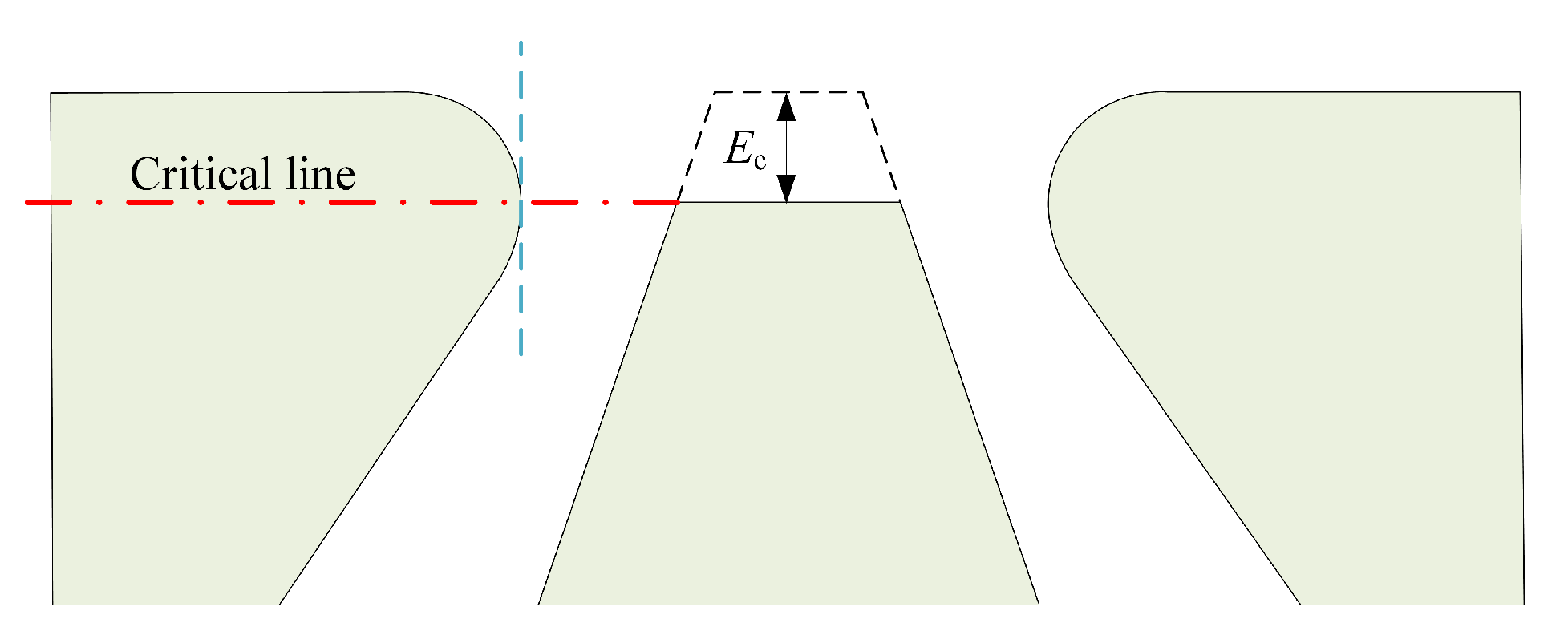
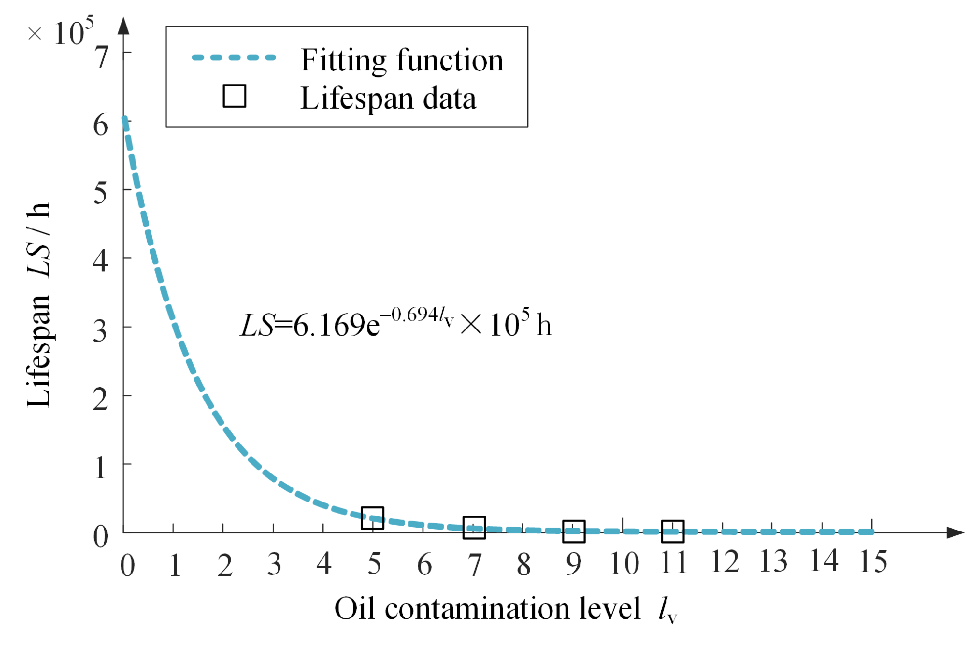
A new failure criterion of DJVs is proposed and the lifespan prediction method is presented, which will aid in balancing the economy and the durability in DJV application.

2. Formulation of Erosion in Pilot Hydraulic Amplifier

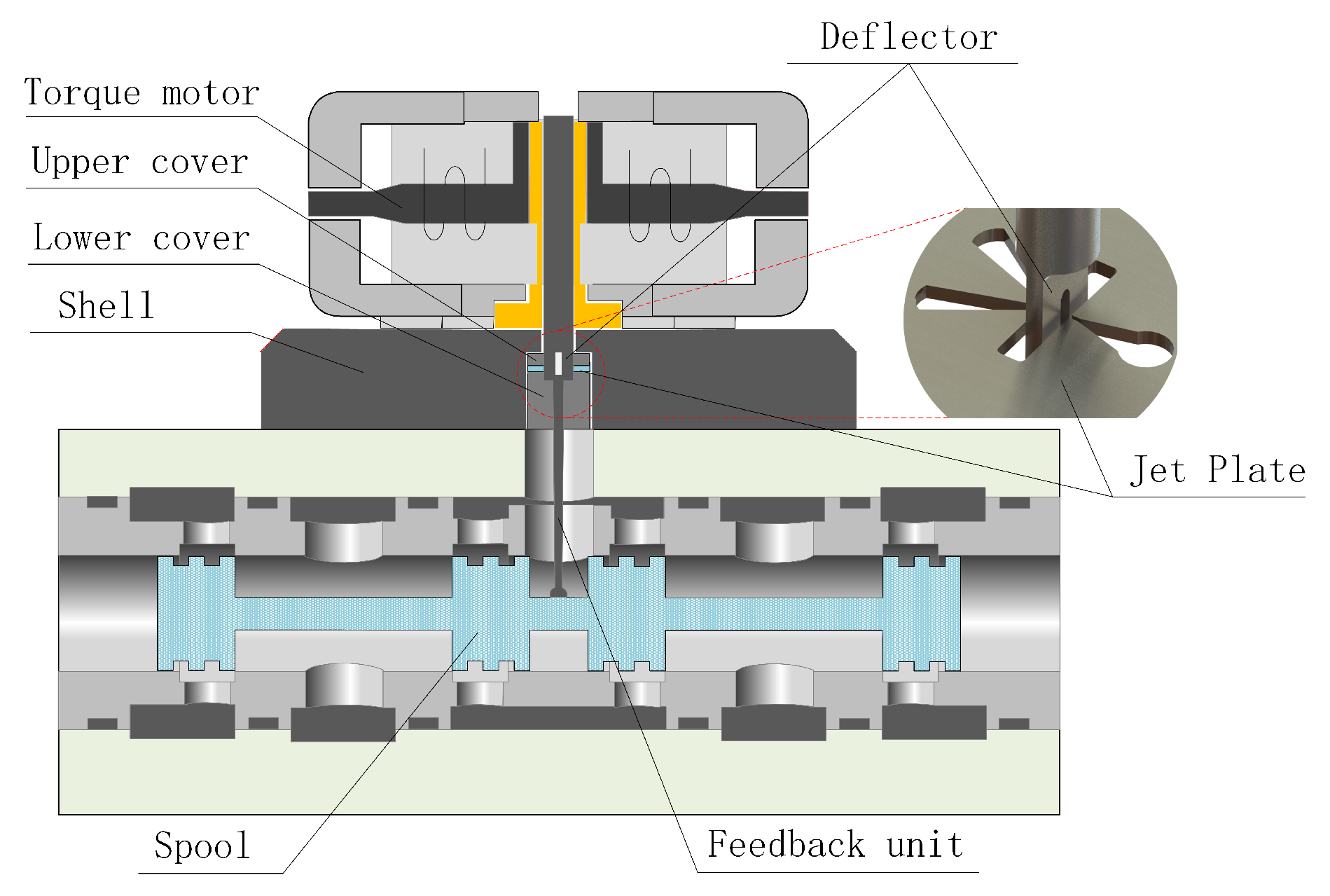
2.1. Mechanism of Hydraulic Amplifier Driving the Spool Valve

In the deflector jet valve, a deflector and a jet plate constitute the deflector jet structure, which acts as a pilot hydraulic amplifier of the valve, as depicted in Figure 1. The jet plate is responsible for generating a high-speed jet and the working pressures in two receivers, while the deflector motion can adjust the jet subtly and manipulate the pressures, driving the spool valve to move. Hence, the hydraulic amplifier is a key power unit that fulfils the mission of spool valve control in cooperation with the feedback unit and the electrical input unit (see Figure 2).

2.2. Erosion Wear in Hydraulic Amplifier

As illustrated in Figure 1, the jet plate and the deflector are confronted with high-speed fluid and varied degrees of impacts between the fluid and the solid walls. Intuitively, significant erosion wear can happen at the places where either high flow velocity or intense impact occurs. Therefore, it can be speculated that the jet orifice of the jet plate, the side walls inside the deflector, the shunt wedge, and the guide curve outside the receiver are most possible to be susceptible to erosion wear, as shown in Figure 3. In respect of the mechanism of erosion wear, since the molecular force of hydraulic oil exerted on the metal surface is much less than the force brought by solid particles in oil, it is assumed that the erosion wear is only caused by continuous particle impacts. That is, because of surface material’s ductility, particle impacts will result in formation of tiny craters and abscission of metal scraps. While the effect of particle impact primarily depends on the material performances of particles and target surfaces, the impact direction, the quantity of impact particles and the distribution of particle sizes [5]. For the specific scenario of servo valves, the size and quantity of particles in oil can be characterized as the contamination level, as listed in

Table 1. Optimized results of the circular arch for different slenderness and opening angles [18].

Number of Particles in 100 mL Oil
Contamination Level	Particle Size Range
	$\mathbf{5}\sim \mathbf{15}$	$\mathbf{15}\sim \mathbf{25}$	$\mathbf{25}\sim \mathbf{50}$	$\mathbf{50}\sim \mathbf{100}$	100
00	125	22	4	1	0
0	250	44	8	2	0
1	500	89	16	3	1
2	1000	178	32	6	1
3	2000	356	63	11	2
4	4000	712	126	22	4
5	8000	1425	253	45	8
6	16,000	2850	506	90	16
7	32,000	5700	1012	180	32
8	64,000	11,400	2025	360	64
9	128,000	22,800	4050	720	128
10	256,000	45,600	8100	1440	256
11	512,000	91,200	16,200	2880	512
12	102,400	182,400	32,400	5760	1024

.

The contamination level of hydraulic oil used in the aerospace industry is 13/11 of an enterprise standard QJ2724.1-2724.7-95 [19], which is approximately equivalent to Level 5 of the NAS standard. In addition, for an actual servo valve, a built-in filter with a precision of 10um is placed before the hydraulic amplifier. As a consequence of that, the actual number of the particles entering the hydraulic amplifier should be below 1% of the original number, which is described as follows [20].

$${\beta }_{10}=N_u/N_d$$

(1)

where $N_u$ and $N_d$ are the numbers per unit volume of particles exceeding 10 um before and after filtering, respectively; ${\beta }_{10}$≥ 100 is the reduction ratio. The material of the deflector and the jet plate is 3J1, with its performance listed in

Table 2. Material Performance of 3J1 [21].

Parameter	Property and Value
Material	3J1
Main chemical constituents (mass fraction)	Ni: 34.5%–36.5%
	Cr: 11.5%–13.0%
	Ti: 2.70%–3.20%
	Al: 1.00%–1.80%
	Fe: the Rest
Tensile strength (N/mm${}^2$)	1372
Density (g/cm${}^3$)	8.03
Vicker hardness (kgf/mm${}^2$)	400–480

.

3. Materials and Methods

A RANS-based CFD method is adopted in this erosion wear investigation. Relevant techniques mainly involve: flow modelling based on the $k-\epsilon$ turbulence model, particle trajectory modelling in the Lagrangian reference frame and erosion rate calculation. The validity of these techniques has been confirmed by [22]. The theories underlying the research methodology are formulated as follows.

3.1. Rans Simulation Method of Fluid

The mass continuity and the momentum conservation in time-averaged form used in flow modelling are expressed by

$$\frac{\partial {\overline{u}}_i}{\partial x_i}=0$$

(2)

$${\overline{u}}_j\frac{\partial \overline{u_i^{{}^{\prime }}}}{\partial x_j}=-\frac{1}{\rho }\frac{\partial \overline{P}}{\partial x_i}+\frac{\partial }{\partial x_j}\left[v(\frac{\partial \overline{u_i^{{}^{\prime }}}}{\partial x_j}+\frac{\partial \overline{u_j^{{}^{\prime }}}}{\partial x_i})-\overline{u_i^{{}^{\prime }}{u}_j^{{}^{\prime }}}\right]$$

(3)

in which the Reynold pressure terms $\overline{u_i^{{}^{\prime }}{u}_j^{{}^{\prime }}}$ are obtained from solutions of the turbulence kinetic energy equations listed as follows [13].

$$\frac{\partial \overline{u_i^{{}^{\prime }}{u}_j^{{}^{\prime }}}}{\partial t}+{\overline{u}}_j\frac{\partial }{\partial x_j}\left(\overline{u_i^{{}^{\prime }}{u}_j^{{}^{\prime }}}\right)=\left(\overline{u_i^{{}^{\prime }}{u}_l^{{}^{\prime }}}\frac{\partial {\overline{u}}_j}{\partial x_l}+\overline{u_j^{{}^{\prime }}{u}_l^{{}^{\prime }}}\frac{\partial \overline{u_j^{{}^{\prime }}}}{\partial x_l}\right)+C_s\frac{\partial }{\partial x_l}\left[\frac{k}{\epsilon }\overline{u_l^{{}^{\prime }}{u}_m^{{}^{\prime }}}\frac{\partial }{\partial x_m}\overline{u_i^{{}^{\prime }}{u}_j^{{}^{\prime }}}+A_{ij}-\frac{2}{3}{\delta }_{ij}\epsilon \right]$$

(4)

where k is the turbulence kinetic energy and $\epsilon$ is the dissipation rate; $A_{ij}$ is the redistributive fluctuating pressure term determined according to [23]. And $\epsilon$ can be governed by

$$\frac{\partial \epsilon }{\partial t}+{\overline{u}}_j\frac{\partial \epsilon }{\partial x_j}=C_{\epsilon }\frac{\partial }{\partial l}\left(\frac{k}{\epsilon }\overline{u_l^{{}^{\prime }}{u}_m^{{}^{\prime }}}\frac{\partial \epsilon }{\partial x_m}\right)-C_{\epsilon 1}\frac{\epsilon }{k}\overline{u_l^{{}^{\prime }}{u}_m^{{}^{\prime }}}\frac{\partial {\overline{u}}_l}{\partial x_m}-C_{\epsilon 2}\frac{{\epsilon }^2}{k}$$

(5)

where $C_{\epsilon }$ = 0.18, $C_{\epsilon 1}$ = 1.44 and $C_{\epsilon 2}$ = 1.90 [23].

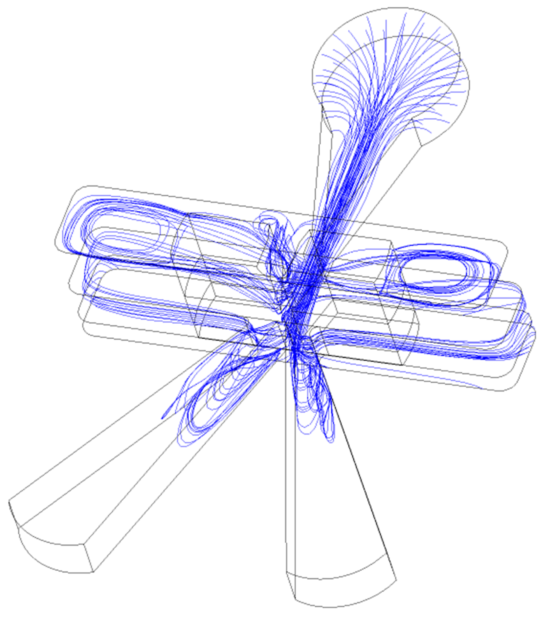
3.2. Particle Trajectory Generation

The trajectory of a discrete phase particle can be calculated by integrating the force balance equations on the particle in the Lagrangian reference frame, expressed as

$$\frac{d\overrightarrow{u}}{dt}=\frac{(\overrightarrow{u}-{\overrightarrow{u}}_P)}{{\tau }_r}+\frac{\overrightarrow{g}({\rho }_P-\rho )}{{\rho }_P}+\overrightarrow{F}$$

(6)

where $\overrightarrow{F}$ is the additional acceleration term due to the reference frame rotation, $\overrightarrow{u}$ is the fluid velocity, ${\overrightarrow{u}}_P$ is the particle velocity, $\frac{(\overrightarrow{u}-{\overrightarrow{u}}_P)}{{\tau }_r}$ is the drag force per unit particle mass, $\rho$ is the fluid density, ${\rho }_P$ is the particle density, and ${\tau }_r$ is the particle relaxation time expressed as [24]

$${\tau }_r=\frac{{\rho }_P{d}_P^2}{18\mu }\frac{24}{C_{d}Re}$$

(7)

where $\mu$ is the molecular viscosity of the fluid and $C_d$ is the drag coefficient computed by [6]

$$C_d=\frac{24(1+b_{1}R{e}^{b_2})}{Re}+\frac{b_{3}Re}{b_4+Re}$$

(8)

where $b_1,b_2,b_3$ and $b_4$ are functions of the particle shape factor. $Re$ is the relative Reynold number, defined as

$$Re=\frac{\rho d_P|\overrightarrow{u}-{\overrightarrow{u}}_P|}{\mu }$$

(9)

in which $d_P$ is the particle diameter.

To account for particle rotation, an additional angular momentum equation is supplemented as

$$I_P\frac{d{\overrightarrow{\omega }}_P}{dt}=\frac{\rho }{2}{\left(\frac{d_P}{2}\right)}^5{C}_{\omega }\overrightarrow{\Omega }=\overrightarrow{T}$$

(10)

where $I_P$ is the moment of inertia, ${\overrightarrow{\omega }}_P$ is the particle angular velocity, $C_{\omega }$ is the rotational drag coefficient, $\overrightarrow{T}$ is the torque applied to the particle and $\overrightarrow{\Omega }$ is the relative particle-fluid angular velocity.

3.3. Erosion Rate Model

According to [9], the erosion rate can be obtained by

$$E_v=f\left(\alpha \right)E_{90}$$

(11)

$$E_{90}=K{\left(H_{vw}\right)}^{k_1}{\left(\frac{u_P}{u^{*}}\right)}^{k_2}{\left(\frac{d_P}{d^{*}}\right)}^{k_3}$$

(12)

$$f\left(\alpha \right)={\left[sin\left(\alpha \right)\right]}^{n_1}{\left\{1+H_{vw}\left[1-sin\left(\alpha \right)\right]\right\}}^{n_2}$$

(13)

in which $\alpha$ is the impact angle; $E_v$ represents the volumetric erosion rate at the impact angle $\alpha$; $E_{90}$ is the erosion rate at a normal impact angle; $u^{*}$ and $d^{*}$ are the reference impact velocity and the reference diameter of the particle, respectively, with the values 104 m/s and 0.326 um; $u_P$ and $d_P$ are the impact velocity and the particle diameter, respectively; $H_{vw}$ is the Vickers hardness of the target material; $f\left(\alpha \right)$ is the correlation between the erosion rate and the impact angle, with dimensionless units. And according to [22], K = 50, $k_1$ = $-0.12$, $k_2$ = 2.3${\left(H_{vp}\right)}^{0.038}$ and $k_3$ = 0.19, where $H_{vp}$ is the Vikers hardness of particles; $n_1$ and $n_2$ depend on the particle type and the target hardness, determined as follows [8].

$$n_1=s_1{\left(H_{vw}\right)}^{q_1}$$

(14)

$$n_2=s_2{\left(H_{vw}\right)}^{q_2}$$

(15)

where $s_1$ = 0.71, $q_1$ = 0.14, $s_2$ = 2.4 and $q_2$ = $-0.94$.

After impact the particle bounces off the wall, which can be estimated or represented using the momentum-based restitution coefficients, with the following assumption [25].

$$\left\{\begin{array}{c}{e}_n=1.0-0.4159\alpha +0.4994{\alpha }^2-0.292{\alpha }^3,\hfill \\ e_t=1.0-2.12\alpha +3.0775{\alpha }^2-1.1{\alpha }^3,\hfill \end{array}\right.$$

(16)

where $e_n$ and $e_t$ are the restitution coefficients in normal and tangential directions, respectively, which are essential for the particle trajectory calculation.

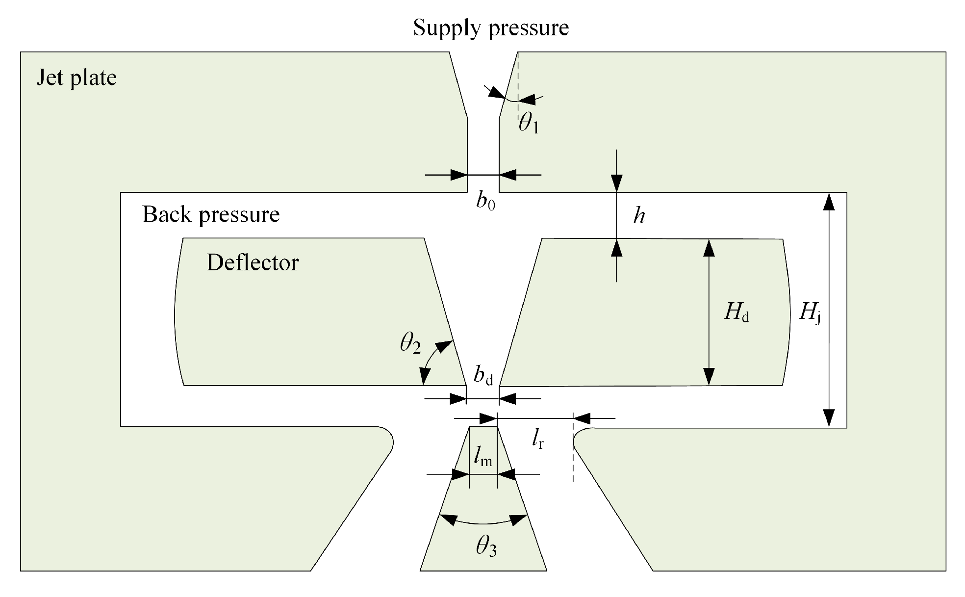
3.4. Numerical Modelling of Deflector Jet Mechanism

By reference to an actual hydraulic amplifier, the geometric parameters of the hydraulic amplifier can be determined by Figure 4 and

Table 3. Values of geometric parameters.

Parameter	Value
Jet orifice width of jet plate $b_0$ (mm)	0.15
Outlet width of deflector $b_d$ (mm)	0.14
Distance between deflector and jet orifice h (mm)	0.18
Distance between jet orifice and receiver $H_j$ (mm)	1
Deflector thickness $H_d$ (mm)	0.64
Receiver width $l_r$ (mm)	0.34
Shunt wedge width $l_m$ (mm)	0.1
Inflow angle ${\theta }_1$ (${}^{\circ }$)	13
Sidewall inclination angle ${\theta }_2$ (${}^{\circ }$)	16.5
Shunt wedge angle ${\theta }_3$ (${}^{\circ }$)	38

. A numerical model has been built as depicted in Figure 5. With an inlet pressure of 21 MPa and an outlet pressure of 0 MPa, a RANS-based CFD simulation can be performed, with relevant simulation parameters listed in

Table 4. Calculation conditions of erosion wear simulation.

Parameter	Value
Densities of oil $\rho$ (kg/m${}^3$)	850
Oil viscosity $\mu$ (kg·s/m)	data
Densities of wall ${\rho }_w$ (kg/m${}^3$)	0.0085
Densities of particles ${\rho }_p$ (kg/m${}^3$)	8030
Average diameter of particles d${}_m$ (mm)	1550
Pressure of inlet $P_{in}$ (MPa)	21
Pressure of outlet $P_{out}$ (MPa)	0
Total flow rate $Q_t$ (kg/s)	$4.1858\times {10}^{-11}$
Shape factor $\varphi$	0.6
Reference erosion rate $K{\left(H_{vw}\right)}^{k_1}$ (kg/kg)	$3.124\times {10}^{-4}$
Wall material Vickers hardness $H_{vw}$ (GPa)	4.0
Material hardness exponents $n_1$	0.8
Particle properties exponents $n_2$	1.3
Velocity exponent $k_2$	2.35
Diameter exponent $k_3$	0.19
Reference diameter $d^{*}$ ($\mathsf{\mu }$m)	0.326
Reference velocity $u^{*}$ (m/s)	104

.

Then the Finite Volume commercial code ANSYS/FLUENT is employed to solve the continuity, momentum, turbulence and discrete phase equations. The simulation is based on the hypotheses of steady-state and incompressible flow, and the second order upwind spatial discretization scheme is employed.

4. Results and Discussion

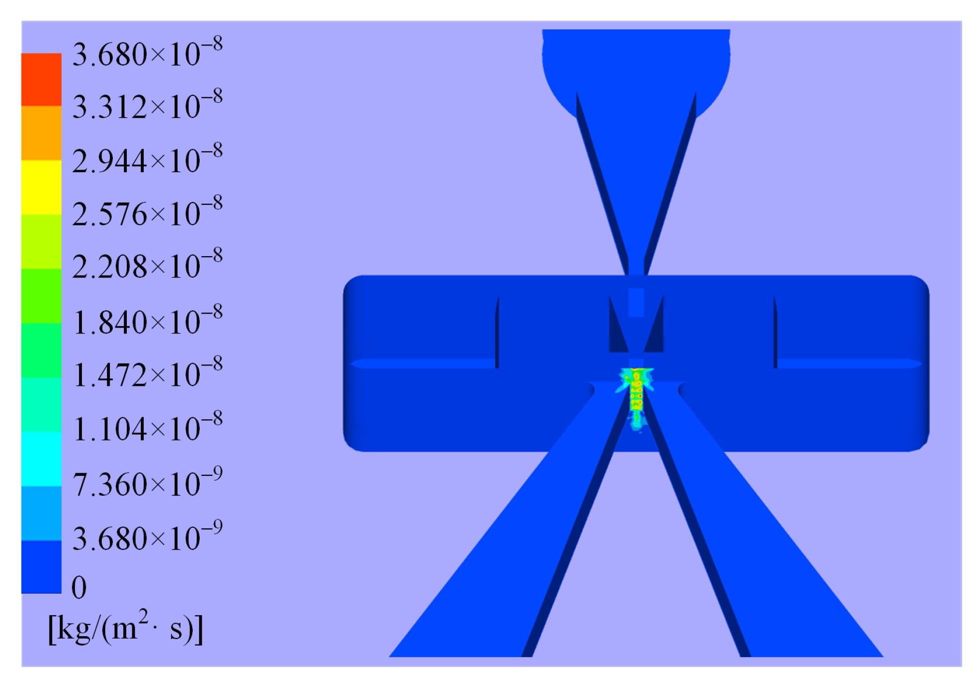
4.1. Distribution of Erosion in Valve

As already mentioned, it is speculated that significant erosion wear is likely to happen at some places confronted with high-speed flow or jet impact. According to the CFD-based simulation, an overall profile of the erosion for oil of NAS 7 is represented in Figure 6, and the particle trajectories are shown in Figure 7. The erosion wear in the hydraulic amplifier can be graded into four levels. The wear of Level 1, with an erosion rate level of 10${}^{-8}$ kg/(m${}^2$·s), appears on the shunt wedge sustaining the major jet impact and some of the receiver surfaces close to the shunt wedge (see Figure 8, Figure 9 and Figure 10). What it means is that the erosion in the vicinity of the shunt wedge will be much more severe than elsewhere and becomes our main concern.

The wear of Level 2 has the erosion rates with an order of magnitude of 10${}^{-9}$ kg/(m${}^2$·s), happening at locations illustrated in Figure 11, Figure 12, Figure 13 and Figure 14. It follows that the effects of erosion on the jet orifice, the side walls of the deflector and the guide curve of the receiver are much less than that on the shunt wedge, although these effects have conformed to previous expectations. Weaker wear is defined as Level 3, with the erosion rate level 10${}^{-10}$ kg/(m${}^2$·s), and happens mainly near the jet orifice, as depicted in Figure 15. In addition, the wear with erosion rates less than 10${}^{-10}$ kg/(m${}^2$·s) is classified as Level 4 and has a minimal effect on the valve.

4.2. Characteristics of Major Erosion Wear

According to the above analyses, the most severe wear appears on the impact sustaining surface of the shunt wedge, with erosion rates depicted in Figure 16. What it means is that the jet impact results in an undulating distribution of the erosion on the shunt wedge. There exist multiple relative erosion rate maximums, but no one is right located at the jet center.

Consider the erosion rate variation along two orthogonal axes on the impact surface, as marked in Figure 15. It can be found the erosion pattern in both directions is the regular fluctuation with a particular wavelength, as shown in Figure 17 and Figure 18.

The wavelengths in the two directions are 0.08 mm and 0.10 mm, respectively. When deviating away from the jet center, the fluctuation amplitude gradually declines. Consequently, the erosion rate distribution is supposed to be created by the interference of the fading erosion fluctuations in the two directions. The formation of this phenomenon may be related to the motion pattern of the high-speed particle beam entering a narrow space.

4.3. Correlation Between Oil Contamination Level and Erosion Wear

As listed in Table 1, the contamination level decides the particle concentration of hydraulic oil. Simulations show that the contamination level plays a remarkable role in the erosion wear of the shunt wedge. According to the erosion rate distribution obtained, after the shunt wedge sustains 1000 h of impact, the erosion depths for different contamination levels are obtained, illustrated by Figure 19, Figure 20, Figure 21 and Figure 22. Without consideration of the erosion rate variation with the impact surface’s change in shape, these calculations based on a linear erosion assumption are approximate.

However, the average erosion depths can be computed, which is obviously significant for giving quantitative wear estimations for different contamination levels. With the increase of the contamination level, the average erosion depth will rise exponentially while its logarithm is approximately linear with respect to the contamination level, as depicted in Figure 23, just in accordance with the particle concentrations defined by contamination levels. Conversely, the valve lifespan can be predicted according to the average erosion depth if a failure criterion is determined.

4.4. Lifespan Predication Based on Erosion Wear

Regarding the DJV, there is still no recognized standard to determine the valve failure, different from the jet pipe valve [16]. Here, a failure criterion is proposed according to an analysis of the pressure generating mechanism in the receiver and its structural characteristics. The jet passing through the deflector impacts on the shunt wedge, and then the fluid will flow along gaps on both sides, with the momentum component perpendicular to the impact surface generating the receiver pressure. After this momentum component depleted, the fluid accomplishes its mission and must return to the reservoir smoothly, which is just the function of the guide curve outside the receiver. Therefore, when the impact surface of the shunt wedge, due to wear, is below the point on the guide curve closest to the shunt wedge, as depicted in Figure 24, the flow parallel to the impact surface will be blocked by the guide curve, resulting in internal eddies becoming much more complicated. As a result, the flow stability will materially deteriorate because of eddy-induced cavitation and vibration, and the reliability of the DJV will significantly decline. Consequently, the critical line in Figure 24 is adopted to evaluate the valve condition, and $E_c$ is the failure depth, with the value 0.08 mm in this case. Meanwhile, by reference to the erosion rates distribution (see Figure 16), the average erosion depth per unit time of the shunt wedge can be obtained. It follows that the lifespan of the DJV can be calculated for different contamination levels, as illustrated in Figure 25. Fitting the lifespan calculations for oil of NAS 5, 7, 9 and 11, a prediction formula can be derived as follows.

$$LS=6.169e^{-0.694l_v}\times {10}^5\left(h\right)$$

(17)

Following this exponential function, the lifespan will increase rapidly with the contamination level promoted. Specifically, to gain a lifespan of over 20,000 h one must employ the hydraulic oil with a contamination lever superior to NAS 5. However, the excessive cleanliness of the hydraulic oil will lead to a sharp increase of economy and time costs, and it is futile to merely prolong the pilot valve life for the whole valve or valve-controlled systems. Therefore, it matters that we first determine a suitable lifespan for the servo valve to adapt to the systematic lifespan demand, and then a requisite contamination level can be chosen according to the predication formula (17).

As already mentioned, the shunt wedge change in shape has been ignored in the erosion depth calculation. In fact, with the erosion wear continuously proceeding, the shunt wedge becomes wider and wider, which means that its capability of sustaining the jet impact will be strengthened. Hence, it may be supposed that the predictions in Figure 25 are relatively safe.

5. Conclusions

According to this investigation, it can be confirmed that the major erosion wear happens on the shunt wedge, and this wear takes on a regular fluctuation, which should be correlative of the large-scale vibration of fluid in the tiny space of the hydraulic amplifier of DJVs. Following and interacting with fluid, particles amplify the effect of this vibration by surface erosion. Since the research is based on the RANS simulation, it follows that transient pressure fluctuations are not considered. Hence, the actual erosion wear may be slightly worse. However, with the erosion wear proceeding, the shunt wedge gradually becomes wider, and this is an unconsidered factor favourable to its anti-erosion capacity. In general, the above factors are far less influential than a slight change of the oil contamination level, which means the proposed methodology and the results acquired can be utilized to estimate the contamination level dependence of the erosion wear effectively.

The exponential growth pattern of the lifespan is actually consistent with the particle concentrations defined by different contamination levels. Generally, a contamination lever of NAS 5 should be guaranteed to obtain about 20,000 h lifespan. However, according to the previous assumption, a premise of this prediction holding is that the built-in filter must be effective and healthy. Although not involved in this paper, the lifespan of this filter should be considered in practical engineering.

References

1. Wellinger, K.; Brockstedt, H.C. Versuche zur Ermittlung des Verschleisswiderstandes von Werkstoffen für Blasversatzsohr sowie des Einflusses der Rohrverlegung bei Blasversatzanlagen. Glückauf 1942, 78, 130. [Google Scholar]
2. Wellinger, K.; Brockstedt, H.C. Ermittlung des Verschleisswiderstandes von Werkstoffen für Blasversatzrohre. Stahl Eisen 1942, 62, 635. [Google Scholar]
3. Wellinger, K.; Brockstedt, H.C. Sandstrahlverschleiss an Metallen. Z. Metallkunde 1949, 40, 361. [Google Scholar]
4. Wellinger, K.; Uetz, H. Verschleissuntersuchungen an Gumi. Z. Ver. Deut. Ingr. 1954, 96, 43. [Google Scholar]
5. Finnie, I. Erosion of surfaces by solid particles. Wear 1960, 43, 87–103. [Google Scholar] [CrossRef]
6. Hamed, A.A.; Tabakoff, W.; Rivir, R.B. Turbine Blade Surface Deterioration by Erosion. J. Turbomach 2005, 127, 445–452. [Google Scholar] [CrossRef]
7. Ahlert, K.R. Effects of Particle Impingement Angle and Surface Wetting on Solid Particle Erosion of ANSI 1018 Steel. Master’s Thesis, University of Tulsa, Tulsa, OK, USA, 1994. [Google Scholar]
8. Oka, Y.I.; Okamura, K.; Yoshida, T. Practical estimation of erosion damage caused by solid particle impact. Part 1: Effects of impact parameters on a predictive equation. Wear 2005, 259, 95–101. [Google Scholar] [CrossRef]
9. Oka, Y.I.; Yoshida, T. Practical estimation of erosion damage caused by solid particle impact. Part 2: Mechanical properties of materials directly associated. Wear 2005, 259, 102–109. [Google Scholar] [CrossRef]
10. Wallace, M.S.; Dempster, W.M.; Scanlon, T.J.; Peters, J.; Mcculloch, S. Prediction of impact erosion in valve geometries. Wear 2004, 256, 927–936. [Google Scholar] [CrossRef]
11. Zhang, X.; Chen, Y.; Yang, W. Erosion of an Arrow-Type Check Valve Duo to Liquid–Solid Flow Based on Computational Fluid Dynamics. Fail. Anal. Preven. 2019, 19, 570–580. [Google Scholar] [CrossRef]
12. Boulanger, A.J.; Wong, C.Y.; Zamberi, M.A.; Shaffee, S.A.; Johar, Z.; Jadid, M. Fines erosion: Turbophoresis can be harmful. J. Comput. Multiph. Flows 2017, 9, 86–102. [Google Scholar] [CrossRef]
13. Zhao, Y.; Zeng, Z.; Ge, S.; Yao, J. Numerical and experimental investigation of erosion by liquid-solid impinging jet. J. Cent. South Univ. Nat. Sci. Ed. 2018, 49, 1289–1296. [Google Scholar]
14. Yin, Y.; Fu, J.; Jin, Y. Numerical simulation of erosion wear of pre-stage of jet pipe servo valve. J. Zhejiang Univ. Eng. Sci. 2015, 49, 2252–2260. [Google Scholar]
15. Chu, Y.; Yuan, C.; Zhang, Y. The erosion wear characters of the jet pipe servo valve. Acta Aeronaut. Astron. Sin. 2015, 36, 1548–1555. [Google Scholar]
16. Chu, Y.; Yuan, C.; Li, C. Durability simulation analysis of jet pipe servovalve. J. Northwest. Polytech. Univ. 2015, 33, 326–331. [Google Scholar]
17. Zhang, S. The Simulation of Erosion on Servo Valve Orifice and Changes of Valve Characteristics on Jet Deflector Servo Valve. Master’s Thesis, Lanzhou Univ. Tech., Lanzhou, China, 2017. [Google Scholar]
18. Lei, T. Contamination control. In Hydraulic Engineering Manual, 1st ed.; Mach. Ind. Press: Beijing, China, 1990; pp. 1736–1737. [Google Scholar]
19. Contamination Control; QJ2724.1-2724.7-95; Aviation Industry Corporation of China: Beijing, China, 1995; pp. 1–5.
20. Technical Specifications for Hydraulic Filters; GB/T20079-2006; General Administration of Quality Supervision, Inspection and Quarantine of the People’s Republic of China: Beijing, China, 2016; pp. 1–2.
21. 3J1 and 3J53 Alloy for Elastic Component; YB/T 5256-2011; Ministry of Industry and Information Technology of People’s Republic of China: Beijing, China, 2012; pp. 1–5.
22. Njobuenwu, D.O.; Fairweather, M. Modelling of pipe bend erosion by dilute particle suspensions. Comput. Chem. Eng. 2012, 42, 235–247. [Google Scholar] [CrossRef]
23. Dianat, M.; Jones, M.F.P. Reynolds stress closure applied to axisymmetric, impinging turbulent jets. Theor. Comput. Fluid Dyn. 1996, 43, 435–447. [Google Scholar] [CrossRef]
24. Gosman, A.; Ioannides, E. Aspects of computer simulation of liquid-fuelled combustors. In Proceedings of the 19th Aerospace Sci. Meeting(AIAA), St. Louis, MO, USA, 12–15 January 1981. [Google Scholar]
25. Sommerfeld, M.; Huber, N. Experimental analysis and modelling of particle-wall collisions. Int. J. Multiph. Flow 1999, 5, 1457–1489. [Google Scholar] [CrossRef]
Figure 1. Hydraulic amplifier.
Applsci 10 01299 g001
Figure 2. Function of hydraulic amplifier in whole valve.
Applsci 10 01299 g002
Figure 3. Erosion areas speculated.
Applsci 10 01299 g003
Figure 4. Definition of geometric parameters.
Applsci 10 01299 g004
Figure 5. Numerical model of the deflector jet mechanism.
Applsci 10 01299 g005
Figure 6. Overall erosion rate distribution in deflector jet mechanism.
Applsci 10 01299 g006
Figure 7. Particle trajectories.
Applsci 10 01299 g007
Figure 8. Erosion rates on shunt wedge.
Applsci 10 01299 g008
Figure 9. Erosion rates of lower surface of the receiver.
Applsci 10 01299 g009
Figure 10. Erosion rates of upper surface of the receiver.
Applsci 10 01299 g010
Figure 11. Erosion rates of jet orifice.
Applsci 10 01299 g011
Figure 12. Erosion rates of the receiver’s guide curve.
Applsci 10 01299 g012
Figure 13. Erosion rates of shunt wedge’s outer surface.
Applsci 10 01299 g013
Figure 14. Erosion rates of the side wall of the deflector.
Applsci 10 01299 g014
Figure 15. Erosion rates close to the jet orifice.
Applsci 10 01299 g015
Figure 16. Erosion rates distribution on the shunt wedge.
Applsci 10 01299 g016
Figure 17. Erosion rates along the y-axis.
Applsci 10 01299 g017
Figure 18. Erosion rates along the z-axis.
Applsci 10 01299 g018
Figure 19. Erosion depth distribution after 1000h for oil of NAS 5.
Applsci 10 01299 g019
Figure 20. Erosion depth distribution after 1000h for oil of NAS 7.
Applsci 10 01299 g020
Figure 21. Erosion depth distribution after 1000h for oil of NAS 9.
Applsci 10 01299 g021
Figure 22. Erosion depth distribution after 1000h for oil of NAS 11.
Applsci 10 01299 g022
Figure 23. Average erosion depth with contamination level increasing.
Applsci 10 01299 g023
Figure 24. Failure criterion of DJV.
Applsci 10 01299 g024
Figure 25. DJV lifespan prediction for different contamination levels.
Applsci 10 01299 g025