Impact of Road Traffic Tendency in Europe on Fatigue Assessment of Bridges


Department of Civil and Industrial Engineering, University of Pisa, 56122 Pisa, Italy
Appl. Sci. 2020, 10(4), 1389; https://doi.org/10.3390/app10041389
Submission received: 12 December 2019
/
Revised: 21 January 2020
/
Accepted: 14 February 2020
/
Published: 19 February 2020
(This article belongs to the Special Issue Assessing and Extending the Service Life of Bridges)
Abstract
:Fatigue load models for road bridges given in the Eurocode EN1991-2 have been calibrated considering real traffic measurements that became available around 1990. Since then, traffic composition has evolved considerably, also considering the issuing of the 96/53/EC Directive, which legitimated member states, on an equal and not discriminatory basis, to allow the circulation of Long and Heavy Vehicles (LHVs). Thus, the appropriateness of fatigue load models to cover also the effects of these vehicles, which are longer, heavier and potentially more damaging than common Heavy Goods Vehicles (HGVs), became an issue. The aim of the study is to assess how the evolution of European traffic influences the fatigue assessment of bridges. To capture the essence of the problem, three different real traffic measurements are compared in terms of fatigue damage: the Auxerre (FR) traffic, adopted to define fatigue load models in EN1991-2; the Moerdijk (NL) traffic, characterized by a high percentage of LHVs; and the Igualada (ES) traffic. To assess the current relevance of fatigue load models LM2 and LM4 of EN1991-2, the aptitude of these models to adequately reproduce the effects caused by LHVs is discussed in detail. The results demonstrate that the Auxerre traffic is still the most onerous; that the Moerdijk traffic is generally more severe than the Igualada traffic, and that the fatigue load models of Eurocode do not require major updates. The study is further supplemented by investigating the suitability of the formulae provided in the Eurocodes for the damage equivalence factors and to express the influence of the total lorry volume on the fatigue damage. In that latter case, the conclusion is that the formulae proposed in the Eurocodes, based on the assumption of a linear fatigue strength curve with constant conventional slope , could lead to erroneous, even unsafe, estimates of the fatigue life, especially when details are characterized by constant amplitude fatigue limit , thus calling for further improvements of the formulae themselves.
1. Introduction
Traffic-load models for road bridges given in the Eurocode EN1991-2 [1] were developed and calibrated on the basis of real traffic data, obtained in the framework of two large experimental campaigns in several European locations in the period 1980–1994 [2,3,4,5,6,7,8].
At that time, even though other traffic measurements were characterized by higher lorry flows, the slow-lane traffic measured in Auxerre (FR) in May 1986, on the A6 Paris–Lyon motorway, was identified as the most relevant, i.e. inducing the greatest effects on bridges.
Moreover, being characterized by a high percentages of articulated lorry typologies and by low percentage of lorries with trailers, the Auxerre traffic composition was also reckoned to be well representative of the expected lorry traffic trends in continental Europe around the 2020s. For this reason, static and fatigue load models included in EN1991-2 [1] are mainly based on it.
That choice has been repeatedly a posteriori validated by modern traffic measurements, carried out by more modern and accurate weighing in motion (WIM) systems and devices [5].
Of course, highly urbanized and/or industrialized areas, typically like the area served by the Boulevard Périférique in Paris (FR) or the area around the marble quarries in Carrara (IT), may be subject to even more intense traffic flow or heavier traffic composition than Auxerre traffic, but such unusual situations require specific studies, which cannot be easily generalized.
It must be underlined that, aiming to improve the organization of the European transportation network, in the year 1996 the European Commission considerably modified the transport policy in the European Union, issuing the 96/53/EC Directive [8]
The 96/53/EC Directive, amended several times, limits the total mass and length of Heavy Goods Vehicles (HGVs) to 44 t and 18.75 m, respectively, but it allows the member states to permit, following equity and non-discrimination criteria, the circulation of the so-called Long and Heavy Vehicles (LHVs). Long and Heavy Vehicles, typically employed in so-called modular transports, are characterized by total mass higher than 60 t and by total length of 25 m and more, clearly exceeding the limitations foreseen for common HGVs.
To reduce transportation costs and polluting emissions, some northern European countries, in particular Sweden, Finland, The Netherlands and Germany, took the most from that possibility, so experiencing a significant increase of the number of LHVs in long-distance traffic. Furthermore, it cannot be excluded that in the near future other countries could take advantage of this opportunity, thus inducing significant changes in the long-distance traffic composition in Europe.
Since LHVs were not included in the Auxerre traffic, their circulation could influence the design of new bridges and even more heavily the assessment of existing infrastructure, potentially producing a disproportionate increase of maintenance and repair costs. The consequences of allowing the circulation of LHVs is thus the subject of several recent studies [9,10,11,12,13,14,15,16,17,18], also aiming to ascertain its potential impact in terms of fatigue damage [19,20,21,22].
The study deals with the impact of LHVs on the fatigue assessment of European road bridges. With this aim, the fatigue effects produced by significant measured traffics are compared in relevant case studies. The comparison is further enriched considering the effects of fatigue load models LM2 and LM4 of EN1991-2 [1], described in Section 3.
For the sake of comparison, three real traffic samples, recorded with suitable WIM devices, have been considered:
- the slow-lane traffic in Auxerre, assumed as reference traffic;
- the slow-lane traffic measured in May 2007 in Moerdijk (NL), on the A16 Breda–Rotterdam motorway, characterized by a high percentage of LHVs;
- the slow-lane traffic recorded in March 2003 in Igualada (ES), on the A2 Madrid–Barcelona motorway.
This comparison is further motivated remarking that Spanish and Dutch traffics were disregarded in EN1991-2 pre-normative studies. In fact, at that time, statistical analyses of the available data demonstrated that:
- the most consistent data in terms of traffic composition, inter-vehicle distances, inter-axles, weight, length and speed of each lorry were those recorded in Italy, France and Germany;
- the Spanish and Dutch data were excessively influenced by the peculiarities of the respective road networks, thus resulting not fully representative of European long-distance traffics; while,
- UK data resulted scarcely expressive of the continental situation.
The outcomes of the study are thus discussed, also demonstrating that fatigue load models of EN1991-2 adequately reproduce the fatigue effects caused by the most severe European traffics, even containing LHVs. In addition, to widen the significance of the study, an updated version of the equations giving the fatigue damage coefficients as functions of the total traffic volume is proposed, discussing its implications with reference to the actual formulation proposed in the Eurocodes (see EN1993-1-9 [23], EN1993-2 [24], EN 1992-1-1 [25], EN1993-2 [26]) and stressing the most influential parameters.
To facilitate the understanding of the text, in Appendix A is reported the basic nomenclature adopted, while in Appendix B are summarized the essential steps of the procedure used to derive equivalent fatigue categories.
2. Real Traffic Measurements
Real-time measurements of lorry and axle weights are very topical issues in the management of bridges and, more generally, of road networks. These measurements are generally carried out by means of suitable WIM devices, located on the road or on the bridge.
Since the heaviest lorries, especially overloaded ones, are among the major sources of degradation and damage of bridges and road pavements, the availability of WIM systems could be a very helpful tool to balance inspection, maintenance and repair costs.
The main aim of a WIM device installation is twofold:
- on the one hand, it gives information about actual traffic, so contributing to refine the assessment and to optimize the planning of the interventions;
The improvements of WIM devices and of measuring techniques are currently the subject of several studies (see, for example, [4,5,6,9,12,29,30,31,32]).
Of course, since traffic loads on bridges are governed only by commercial vehicles weighing more than 35 kN, the possible presence of cars and light vehicles can be generally ignored in the verifications.
In the following, after a preliminary illustration of the main characters of the long-distance European traffic measurements taken into account to derive load models of Eurocode [1], the most important features of Moerdijk and Igualada traffics are summarized. Additional details can be found in [2,6,19,33,34].
2.1. European Traffic Measurements in Background Studies of Eurocodes
Besides Auxerre, the most important long-distance motorway traffics considered in the development of the Eurocode were recorded in France, on the A1 motorway between Paris and the Roissy Airport in Garonor; in Germany, on the A61 motorway near the Brohltal bridge; and in Italy, on the A1 motorway, in three locations: Fiano Romano, near Roma, Sasso Marconi, near Bologna, and Piacenza.
The measured flows on the slow lane in these locations resulted in the range lorries per day, but measured flows on main roads or secondary roads were markedly lower: lorries per day on main roads; and lorries per day on secondary roads.
Representative parameters of the aforementioned traffics: daily flow; mean value; maximum value and standard deviation of axle loads and total lorry loads are summarized in Table 1 and Table 2, respectively.
Moreover, the study of the available data proved that:
- HGV long-distance continental European traffic is satisfactorily homogeneous;
- over time, in long-distance European traffic:
- ○
- the percentage of articulated lorries tends to increase, opposite to a significant reduction of the percentage of lorries with trailers, which are commercially less profitable;
- ○
- due to more rational management of lorry fleets, the percentage of empty lorry trips descends, thus raising the mean vehicle loads;
- ○
- the percentage of single lorries, increasingly used on local routes declines;
- as expected, long-distance traffics are much heavier than local traffics;
- daily maxima of axle-loads and total weight of vehicles largely exceed the values legally admitted; to all appearances, the ceiling on overloads depends only on the mechanical strength of the vehicles;
- statistical distribution of the axle-load is generally unimodal, the mode being around 60 kN;
- statistical distribution of the total weight is often bimodal, with the first mode around 150 kN and the second mode around 400 kN;
- mean values of axle-load and total weight of heavy vehicles are strongly dependent on the traffic typology, i.e., on the road classification, and are very scattered;
- daily maxima values are much less sensitive to traffic typology: they are in the range 130–210 kN for single axles, in the range 240–340 kN for two axles in tandem, in the range 220–390 kN for three axles in tridem, and in the range 400–690 kN for the total lorry weight.
It must be also underlined that, as consequence of specific industrial choices of lorry manufacturers, HGV geometries adopted in 1980s practically have remained unchanged until now and the sole remarkable innovation concerns the introduction of LHVs.
2.2. The Moerdijk (NL) Traffic
As already remarked, the introduction of LHVs besides giving new prospects for traffic management, could also overcharge the bridges, causing a disproportionate increase of costs.
In the Netherlands, wide campaigns of in situ measurements concerning typical LHV traffics are in progress.
As anticipated, for the aim of the present paper, the measurements carried out in the first week of April 2007 in Moerdijk (NL), on the Breda–Rotterdam motorway, have been considered [22]. These measurements, concerning typical Dutch LHV traffic, characterized by a flow of about 8100 lorries per day on the slow lane, were carried out in the framework of studies regarding the assessment of equivalent fatigue loads for bridge decks.
In [20] commercial lorries in Moerdijk traffic have been classified in the 53 relevant subclasses illustrated in Figure 1.
These subclasses are characterized by a number of axles varying between two and nine, but records contain also lorries with up to 13 axles. The maximum recorded lorry load resulted in being about 1140 kN, pertaining to a 10-axle lorry type O13411, 19.5 m long.
Since the reliability of measurements is not granted when the vehicle speed is too high, vehicles characterized by have been disregarded. Subsequently, physical coherence of measured data have been checked, eliminating lorries characterized, for example, by unrealistic values of the first axle load, not compatible with the steering function of the first axle, or by excessive inter-axle distance; or by excessive length.
Referring to two-axle lorries, some examples of clearly unrealistic recorded data are summarized in Table 3.
Disregarding these very extreme data, the maximum recorded tandem axle load was about 292 kN, pertaining to the tandem axle of the trailer of a T12O3 lorry, whose total weight was 636 kN, while the maximum equivalent uniformly distributed load was about 63 kN/m, pertaining to a T12O21 lorry weighing 813 kN in total.
2.3. The Igualada (ES) Traffic
The significant long-distance Spanish traffic examined in the present study is the aforementioned traffic recorded in March 2003 on the A2 Madrid–Barcelona motorway in Igualada (ES), around 65 km North-West of Barcelona.
The recorded flow on the slow lane was around 5000 lorries per day.
More precise investigation of the recorded data confirmed daily maxima around:
- 200 kN for single axle load;
- 340 kN for tandem axle load;
- 320 kN for tridem axle load;
- 580 kN for total lorry weigth.
2.4. Comparison of Traffic Data
As discussed below, a preliminary phase of the study regarded the critical comparison of the main features of the traffic measurements considered.
First of all, the analysis of the aforementioned traffic measurements demonstrated that long-distance traffic composition in continental Europe is nowadays much more homogenous than in the past, because, actually, the main characteristics of Spanish and Dutch traffics are also in line with those of Auxerre traffic.
Besides, it emerges clearly that the average number of axles per lorry tends to increase: in fact, it rises from around 3.7 in the Auxerre traffic, to around 4.14 in the Igualada traffic, to 4.35 in the Moerdijk traffic.
In order to enhance the significance of the comparison, the relative frequencies of axle loads, ; tandem axle loads, ; tridem axle loads, , and total weight of lorry are reported in the bar chart diagrams of Figure 2a–d, respectively. In the diagrams, Auxerre data are in yellow ochre, Igualada data in violet and Moerdijk data in red. However, considering that comparison in terms of total weight could be misleading when it refers to lorries characterized by different lengths and that the equivalent uniformly distributed load (), obtained dividing the total weight of the vehicle by its total length, is more coherent information, an additional bar chart diagram is reported in Figure 2e, illustrating relative frequencies of .
Inspecting the diagrams, it can be remarked that:
- distribution of axle loads is unimodal for Igualada traffic (mode around 55 kN); bimodal for Moerdijk traffic (first mode, not particularly manifest, around 45 kN; second mode around 60 kN); tetra-modal for Auxerre traffic (first mode around 15 kN, corresponding to light unloaded vehicles, second mode around 65 kN; third and fourth mode, not particularly marked, around 110 kN and 150 kN, respectively;
- distributions of axle loads of Igualada and Moerdijk traffics are characterized by similar upper tails, while that concerning the Auxerre traffic is much more significant;
- distributions of tandem axle loads are always bimodal: for Igualada traffic, the first mode is around 65 kN, the second mode, not particularly marked, is around 210 kN; for Moerdijk traffic, the two modes are around 45 kN and 100 kN, respectively; for Auxerre traffic, the first mode is around 110 kN, the second mode is around 180 kN;
- distributions of tandem axle loads of Igualada and Auxerre traffics are characterized by similar upper tails, well pronounced even beyond 250 kN; while that concerning the Moerdijk traffic is much less evident;
- except for Igualada traffic, distributions of tridem-axle loads are generally unimodal: the mode of Moerdijk traffic is around 150 kN; the mode of Auxerre traffic is around 330 kN;
- distribution of tridem-axle loads of Igualada traffic is tri-modal: the first mode is around 105 kN, the second and third mode around 170 kN and 210 kN, respectively;
- distributions of tridem-axle loads are characterized by clearly different upper tails: Auxerre traffic exhibits the most relevant one, followed by Moerdijk traffic and then by the Igualada traffic, characterized by the lowest;
- distributions of total weights for Igualada and Moerdijk traffic are bimodal: for Igualada traffic, the first mode is around 190 kN, the second mode, not particularly marked, is around 320 kN; for Moerdijk traffic, the first mode is again around 190 kN, the second mode is around 410 kN;
- distributions of total weights for Auxerre traffic is tri-modal: the first mode is around 30 kN, corresponding to light unloaded vehicles, the second mode, not particularly evident, is around 250 kN, the third mode is around 440 kN;
- distributions of total weights of Moerdijk and Auxerre traffics are characterized by similar upper tails, even if the one of Moerdijk is much more extended due to the presence of a small percentage of weighty LHVs, while that regarding Igualada is less pronounced; finally,
- distribution of is unimodal for Igualada traffic, with the mode around 12 kN/m; bimodal for Moerdijk traffic, with the first mode again around 12 kN/m and a second mode, marked weekly, around 28 kN/m; tri-modal for Auxerre traffic, with the first and the second mode, not particularly evident, around 12 kN/m and 32 kN/m, respectively, and the third mode around 45 kN/m;
- distributions of for Igualada and Moerdijk traffics are very similar, the upper tail being more pronounced in the case of Moerdijk traffic; on the opposite, the distribution of of Auxerre traffic is manifestly more heavy, with the upper tail extending well over 60 kN/m;
- total weight of lorry vehicles LHVs could attain very high value, but usually this level is associated with axle loads not beyond the legal limit;
- as clearly perceptible comparing distributions, Moerdijk traffic appears, in general, less demanding than Auxerre traffic, despite the fact that occasionally axle loads can be higher;
- excluding tandem-axle load distributions, which appear not dissimilar, Igualada traffic looks, in general, lighter than Auxerre traffic;
- apart from tandem-axle load distributions, Moerdijk traffic results, in general, moderately heavier than Igualada traffic.
On the basis of these remarks, it seems confirmed that Auxerre traffic composition stands for a kind of upper limit for actual European traffic. Moreover, the fact that Auxerre data were probably systematically overestimated, since they were obtained by means of past-generation WIM devices less accurate than the updated ones available of today, contributes to further strengthening the conclusion.
Consequently, although this aspect is out of the scope of the present paper, it seems that static load models of EN1991-2, based on Auxerre traffic, are able to represent not only Igualada but also Moerdijk traffic effects, thereby confirming, at this stage, its effectiveness. However, to draw more definitive conclusions deeper specific studies are still necessary.
3. Fatigue Load Models
To discuss the impact of the three considered traffics on fatigue assessment of steel details of road bridges, some relevant case studies have been considered, varying the bridge scheme and the span, as described in detail in Section 4.
Besides real traffics, to measure the differences in terms of results of conventional fatigue assessment, also the notional fatigue load models of EN1991-2, LM2, “set of standard lorries”, and LM4, “set of equivalent lorries”, briefly described in the following, have been taken into account. In fact, these fatigue load models, although accurately calibrated on the basis of Auxerre traffic, are generally a little on the safe side.
EN1991-2 [1] (note 2 of §4.6.1(2), items c and e, explicitly states that use of road bridges’ fatigue load models no. 2 and no. 4 is allowed only when “the simultaneous presence of several lorries on the bridge can be neglected. If that is not the case, they should be used only if they are supplemented by additional data.”
To account for the simultaneous presence of lorries on the same lane, artificial traffic samples have been generated starting from LM2 and LM4 sets of vehicles. These artificial traffics have been generated using a Monte Carlo algorithm, specifically developed [35] and suitably adapted via the Latin hypercube sampling technique [36]. In the algorithm, the analytical probability that two vehicles are simultaneously travelling the lane is explicitly considered, according to [35].
Since the comparison mainly focuses on the effects of traffic composition, an identical value of the total lorry flow has been adopted for all the considered traffics.
Fatigue Load Models LM2 and LM4 of Eurocode EN1991-2
The Eurocode EN1991-2 provides five load models for fatigue verifications of road bridges.
Fatigue load model no. 1 (LM1), derived from the main model used for static verifications, is a very rough and simplified fatigue model intended to assess unlimited fatigue life. This model is out of the scope of the present study, therefore it will not be discussed further.
Fatigue load model no. 3 (LM3) is a simplified model for fatigue damage calculations, which is described in the following Section 5.
Fatigue load model no. 5 (LM5), which is the most general one, consists of a representative real traffic sample directly derived from traffic registrations. Evidently, in the present case LM5 represents, in turn, one of the three traffic measurements.
Fatigue load model no. 2 (LM2) is intended to assess whether fatigue life is limited or not, therefore it can be used only when a constant amplitude fatigue limit exists, like for steel details. Fatigue load model no. 4 (LM4) is specifically devoted to damage calculations.
It must be remarked that LM2 and LM4 are notional models, which have been calibrated with different purposes, as explained later. For that reason, to avoid inconsistencies they should be applied in sequence. In any case, it should be borne in mind that compliance with fatigue verification for unlimited fatigue life, if relevant, automatically implies that fatigue damage cannot occur, as explained better in the following.
In fact, if exists, LM2 should be used first. Said the partial factor on fatigue actions; the partial factor on fatigue resistance and the maximum stress range caused by LM2, if it results as:
the fatigue verification is satisfied and no further verification is needed.
If Inequality (1) is not verified, the fatigue damage should be assessed using LM4 and the Palmgren–Miner formula [35,36]:
where is the number of cycles in the stress spectrum at stress range, the number of cycles to failure at ; and the summation is extended to all cycles for which , being the cut-off limit.
Evidently, as already remarked, when verifications are carried out using both LM2 and LM4, while Inequality (2) implies Inequality (1), the opposite seems not always be true; but this contradiction is not real, since is a threshold for fatigue damage: if the maximum stress range is below that threshold, it cannot cause fatigue damage. The general statement is that the fatigue assessment is governed by the most favorable, or the less onerous, between Inequalities (1) and (2).
It must be stressed that, according to the basic hypotheses of the Eurocodes, characteristic fatigue strength curves are considered in the present study.
The characteristic curve corresponds to the lower bound of the prediction interval 5%–95%, i.e., 5% probability of failure. It is obtained by a downward vertical translation of two standard deviation of the mean curve.
Fatigue load models LM2 (Figure 3) and LM4 (Figure 4) are sets of standardized lorries, representing the most common axle arrangements of European lorries, characterized by “frequent” (LM2) or “damage equivalent” (LM4) values of axle loads.
The axles of the standardized lorries are distinct in three typologies: A; B; C; depending on the dimensions of the contact surface of the wheels, as illustrated in Figure 5. In Figure 3 and Figure 4, the axle types are indicated in the last column.
It must be recalled that, in the framework of EN1991-2 pre-normative studies:
- LM2 was calibrated referring to a kind of “frequent” value , representing the maximum stress range relevant for unlimited fatigue life assessment. This “frequent” value was calculated according to two alternative definitions as:
- ○
- the stress range exceeded about times during the notional design life of the structure; or, alternatively,
- ○
- the stress range corresponding to 99% of the total fatigue damage, calculated considering a curve with constant slope , i.e.,which means that damage produced by stress ranges is practically negligible;either way obtaining comparable values.
Depending on the relevance of the route concerned and on the road category, in fatigue load model LM4 three different reference traffics are considered: long-distance; medium-distance; and local traffic, characterized by different traffic compositions. That accounts for the actual policy of optimal management of commercial lorries: in fact, bigger and heavier vehicles are increasingly used in long-distance traffic, preferably devoting lighter and quicker vehicles to medium-distance and local traffics. Of course, long distance traffic is more severe than medium distance traffic and medium distance traffic is more severe than local traffic composition.
A rather obvious, but extremely important remark is that axle loads and total weights of standardized lorries are beyond the legal limits not only in LM2, but also in LM4; in fact:
- the maximum axle load is 190 kN in LM2 and 270 kN in LM4; while the legal limit is 120 kN;
- the maximum tandem axle load is 280 kN in LM2 and 240 kN in LM4, while the legal limit is 200 kN;
- the maximum tridem axle load is 360 kN in LM2 and 270 kN in LM4, while the legal limit is 240 kN;
- the maximum vehicle weight is 630 kN in LM2 and 490 kN, while the legal limit is 440 kN.
Recalling the previous discussion about measured traffics, this is not surprising, being just a pragmatic acknowledgment of the real situation, but it further demonstrates the relevance of the subject.
4. Case Studies
Aiming to discuss fatigue effects caused by different traffics and fatigue load models, three case studies have been considered, corresponding to particularly relevant influence lines:
- case study no. 1: bending moment at midspan of a simple supported beam (Figure 6a);
- case study no. 2: hogging moment at the intermediate support of a two-span continuous beam having constant bending stiffness (Figure 6b);
- case study no. 3: bending moment at midspan of a three-span continuous beams with span ratios 0.8:1.0:0.8, having constant bending stiffness (Figure 6c).
In each case, the length of the main span has been hypothesized varying in the interval 1–200 m, more precisely assuming the discrete values:1; 3; 5; 8; 15; 30; 50;75; 100; l50 and 200 m.
4.1. Assessment of Fatigue Effects
For each case study and for each value of the span length considered in the study, the bending moment histories produced by Auxerre, Moerdijk and Igualada traffics as well as by the fatigue load models LM2 and LM4 have been determined.
As anticipated, the possibility that two vehicles were simultaneously travelling at the same lane, has been properly taken into account, when relevant.
Regarding LM4, coherently with the features of real traffic measurements considered here, long-distance compositions have been adopted.
In the analyses, fatigue effects have been assessed considering two distinct subcases, depending on the shape of the curve:
- Subcase 1, which deals with details and materials endowed with constant amplitude fatigue limit; like most of the structural steel details (EN1993-1-9 [23]), characterized by fatigue resistance bilinear or trilinear characteristic curves;
- Subcase 2, which deals with details and materials characterized by bilinear characteristic curves, lacking constant amplitude fatigue limit.
curves typically adopted in subcase 1 are illustrated in Figure 7a,b. They are characterized in the bi-logarithmic plane by two or three linear branches:
- when the assessment refers to unlimited fatigue life, a bilinear curve is adopted for steel details. The slope of the inclined branch is commonly assumed [23], but only the horizontal branch, whose ordinate is the constant amplitude fatigue limit , corresponding to cycles to failure, is significant for the verification (Figure 7a);
- when, instead, the assessment requires calculation of fatigue damage, the trilinear curve is adopted, characterized by two inclined linear branches; for steel details, the slopes of the branches are , for , and , for , where , corresponding to cycles to failure, is the so-called cut-off limit, given by the ordinate of the horizontal branch (Figure 7b).
Bilinear fatigue resistance curves typically adopted in subcase 2 are characterized by two inclined branches.
According to Eurocodes [23,26], the slopes of the two linear branches of these curves are and and the abscissa of the knee is cycles (see Figure 7c).
In the present study, it has been assumed that and (see Figure 7d) to match the assumptions adopted in the calibration of fatigue load models of Eurocodes (see, for example, [33]), but it is also the case of some reinforcing steel details [25,26].
Evidently, provided that the slopes of the inclined branches and the abscissas of the knees, i.e., the number of cycles to failure corresponding to the knees, are preset, the curve can be univocally determined by means of one parameter in both the aforementioned subcases. This parameter is the so-called fatigue category of the detail.
For structural steel details, represents the fatigue resistance, expressed in MPa, at cycles, characterized by 95% probability of exceedance; for reinforcing and pre-stressing steel details, represents the fatigue resistance at cycles, characterized by 95% probability of exceedance, or, in other words, the ordinate of the knee of the curve.
The aforementioned representations of the fatigue resistance are strictly valid when the fatigue resistance does not depend on the mean stress of the cycles; but they can be easily generalized, if parameterized in terms of mean stress. Incidentally, it can be observed that, when the effect of mean stress is significant, fatigue loads should be applied starting from the quasi-permanent combination of actions.
4.2. Equivalent Fatigue Categories
In the analyses, the verifications have been carried out both in terms of unlimited fatigue life as well as in terms of fatigue damage, according to the previously anticipated criteria.
Regarding real traffics, the “frequent” value has been determined, according to the already recalled Eurocode pre-normative studies, by using Equation (3).
The fatigue damage, when relevant, has been calculated via the aforementioned Palmgren–Miner law [43,44] (Equation (2)).
For the sake of the comparison, an equivalent, but more expressive, format for fatigue verification can be introduced, in terms of detail category:
where is the actual detail category and the minimum detail category satisfying fatigue verifications.
For details which do not manifest constant amplitude fatigue limit, obviously, this results in:
being the detail category for which the Palmgren–Miner law provides unit fatigue damage . Since, as already said, the definition of fatigue category in the Eurocodes is not univocal, depends on the detail. In fact,
- when detail category is the fatigue strength at cycles:
- ○
- the abscissa of the knee of the curve is located at cycles;
- ○
- and ;
thus is the solution of the equation: - whereas, when the detail category corresponds to the fatigue strength at cycles to failure, like in case of pre-stressing or reinforcing steel details:
- ○
- the abscissa of the knee of the curve is located at ;
therefore, is the solution of the equation:
On the contrary, for details characterized by constant amplitude fatigue limit, this results in:
where is the detail category for which ; is the already recalled maximum stress range relevant for unlimited fatigue life assessments and is the already defined detail category for which it results in .
In the case of structural steel details, since
- ; ;
- the detail category is the fatigue strength at cycles;
- the abscissas of the knees of the curve are at cycles and cycles, respectively;
It results in:
so that is the solution of the equation:
where is the cut-off limit, expressed in terms of .
Notably, in this way the fatigue effects caused by a variety of traffics or fatigue load models can be compared through the associated with each of them, bearing in mind that fatigue effects increase as increases. In this sense, can be interpreted as a measure of the traffic demand in terms of fatigue resistance.
On these premises, to give prominence to the comparison, an equivalence factor can be introduced, which is the ratio between the minimum detail category required by the real traffic considered or by the given fatigue load model, and the minimum detail category required by the Auxerre traffic:
Clearly, values of equivalence factors remain unaltered if internal forces, instead of stresses, are introduced in Equation (11). For example, for elements in bending like those analyzed here, Equation (11) can be rewritten as:
with obvious symbolism.
In conclusion, an equivalence factor plot represents a very synthetic, but eloquent, representation of the fatigue resistance demand of a given traffic, in comparison with the fatigue resistance required by the Auxerre traffic.
From this point of view, is also a tool to directly compare fatigue effects of different traffics or load models, since bigger fatigue effects correspond to higher values of . Anyhow, to better clarify the meaning of and the interpretation of the diagrams, it is useful to point out that the implications of depend on the investigated situation: in fact,
- if the inequality holds for a real traffic, it implies that the real traffic is less demanding than Auxerre traffic; therefore, considering the Auxerre traffic instead of the actual traffic would lead to results on the safe side; on the contrary,
- if the inequality holds for a fatigue load model of EN1991-2 [1], it implies that the load model is less demanding than Auxerre traffic: in this case, the load model underestimates the effects of the Auxerre traffic.
In the study, the total lorry flow in the notional fatigue life of the bridge has been generally set as equal to lorries, in line with recommendations of EN 1991-2 for main roads and motorways subject to intense traffic; but, sometimes, to check the sensitivity of the results on the total flow, also cases with smaller flows have been explored.
It is pleonastic to point out that numerator and the denominator in Equations (11) or (12) have been evaluated adopting curves having the same shape.
It must be also recalled that, in line with their logical bases, fatigue load model no. 2 (LM2) and Equation (8) can be properly applied only when constant amplitude fatigue limit exists (subcase 1).
4.3. Outcomes of the Analysis and Discussion
Following the procedure described before, the appropriate equivalence factor curves have been determined for each case study, distinguishing the two subcases for fatigue resistance curves already identified in Section 4.1.
The outcomes of the analysis are summarized in Figure 8, Figure 9 and Figure 10 for the three case studies, referring to a total flow of lorries.
More precisely, Figure 8 considers bending moment at midspan of simply supported beams (case study no. 1); Figure 9 refers to the hogging moment at intermediate support of two-span continuous beams (case study no. 2) and Figure 10 refers to the bending moment at midspan of three-span continuous beams (case study no. 3).
In the figures, (a) refers to subcase 1 and (b) to subcase 2. To improve the readability of the diagrams, curves concerning fatigue load models of EN1991-2 are in blue; curves concerning Moerdijk traffic are in red; curve concerning Igualada traffic are in green.
Figure 11 refers again to case study no. 1, but assuming the total lorry flow limited to lorries, which is a common situation for roads with low flow rate of lorries. In EN1991-2, for example, annual flows of and lorries, respectively, are given for main roads and secondary roads with low flow rate of lorries.
With this low lorry flow, similar results have been obtained also for case studies no. 2 and no. 3, so it seems unnecessary further discussion about.
Inspecting the curves, it can be remarked that:
- if curves are as per Figure 7c,d, i.e., details do not manifest constant amplitude fatigue limit (subcase 2), fatigue load model LM4 leads in all considered case studies to estimations of the fatigue life on the safe side;
- on the contrary, if curves are as per subcase 1 (Figure 7c,d), i.e., details are characterized by fatigue limit, fatigue load models of EN1991-2 could result in being slightly on the unsafe side in comparison with Auxerre traffic, when and high flow rate is assumed, i.e., the total lorry flow is lorries. In any case the error is generally smaller than 8%, except in case study no. 2 for (Figure 9a), when it attains about 15%.But, in the latter circumstance, besides observing that elements characterized by are rather uncommon, it should be highlighted that the differences are emphasized by the particular shape of the influence line considered in case study no. 2 (Figure 6b): in fact, when the typical inter-axle distances of tandem axles are close to the distance between the two absolute minima of that influence line, .In the other cases, the discrepancies can be explained considering that, in the particular context of and high flow rate, the assessment is governed by the set of “frequent” lorries included in fatigue load model LM2. In fact, in such a condition, the unavoidable differences that exist between standardized lorries and actual lorries, in terms of axle loads; vehicle weight; inter-axle distances of tandem and tridem axles, clearly maximize their effects.
- Fatigue load models are particularly on the safe side when is around 100 m.In that area, the fatigue assessment is certainly governed by the set of “equivalent” lorries given in LM4, but also interactions between consecutive vehicles traveling simultaneously the lane can be significant. The hypothesis that two consecutive lorries are both belonging to the standardized set of LM4 is thus evidently on the safe side, because the probability that the weights of consecutive lorries are regularly close to the equivalent values, which are in some cases outside the legal limits, is small.
- In any case, fatigue load models LM2 and LM4 of EN1991-2 generally reproduce very satisfactorily the fatigue effects induced by Auxerre traffic, so confirming the validity of pre-normative studies and the substantially accuracy of Eurocode fatigue models.
- As the total lorry flow decreases, increases and fatigue load models EN1991-2 tend to be constantly on the safe side (Figure 11).
- The curves associated with curves as per subcase 1 are generally below curves associated with curves as per subcase 2, but the differences become practically insignificant when is high, since for large value of the fatigue assessments depend on fatigue damage.
- Referring to Moerdijk and Igualada traffics and high global flow, the curves associated with subcase 1 are over the curves associated with subcase 2. In fact, contrary to what happens considering Auxerre traffic, in that field the minimum detail categories (Equation (8)) required by Moerdijk and Igualada traffics basically depend on the equivalent stress ranges , rather than on .
- In comparison with Igualada fatigue effects, those evaluated using EN1991-2 fatigue load models are always sensibly on the safe side.
- Moerdijk traffic is constantly less demanding than the Auxerre traffic, except for high global traffic flow in case study 2, subcase 1 (Figure 9a) when , when it results in ;Nonetheless, for , factors associated to Moerdijk traffic substantially results ; moreover tends to slightly reduce as the total flow decreases.
- Considering high flow rate and curves as per subcase 1:
- Considering low global flow, if , Moerdijk traffic composition is always less damaging than the Igualada traffic composition (Figure 11a,b).
- It can be remarked that, for a high value of , Moerdijk traffic looks generally more demanding than Igualada traffic in all examined cases.
- The differences between Moerdijk and Igualada traffics just pointed out can be rationally explained recalling the previous discussion about axle loads and total lorry weight distributions (see Section 2.4).
- Since curves pertaining to the fatigue load models LM2 and LM4 of EN1991-2 are constantly above the curves pertaining to Moerdijk and Igualada traffics, LM2 and LM4 always cover the fatigue effects induced by the non-Auxerre traffics.
It must be underlined that sometimes, when curves are characterized by constant amplitude fatigue limit (subcase 1), the use of fatigue load models LM2 and LM4 could lead to some apparently incoherent results in the transition area, which separates the region where the fatigue assessment is governed by LM2 from the region where the fatigue assessment is governed by LM4. The reason is that axle loads of LM2 and LM4 are sharply different. In fact, these discrepancies sensibly reduce considering real traffics.
5. Damage-Equivalence Factors
In the damage-equivalent factors method, also referred to as the method, the fatigue verification is carried out by means of an “equivalent” static verification.
The rationale of the method is to define an equivalent constant amplitude stress history reproducing the actual fatigue damage . In principle, there are infinite stress histories able to assure that equivalence; in fact, given , it is possible to derive the number of cycles to failure from the stress range of each cycle and vice versa but, fixing conventionally a reference value for one of the two parameters, the other parameter results in being univocally determined.
In the Eurocodes, the equivalence has been established considering as reference value the number of cycles to failure identifying the fatigue category. Therefore, for structural steel details the reference value is cycles and for reinforcing steel and pre-stressing steel details it is (see Section 4.2). The verification consists thus in comparing a suitably calculated “equivalent” stress range, , with the fatigue category of the detail:
The most general expression of the “equivalent” stress range, , is:
where is an additional amplification factor for fatigue verifications, which takes into account, if relevant, dynamic effects, is the basic stress range to be considered, and is the damage equivalent factor. Obviously, in Equation (14) it is:
being the damage equivalent factors, accounting for the most relevant effects influencing the fatigue verification. According what was discussed in Section 3 about fatigue load models LM2 and LM4, for details characterized by constant amplitude fatigue limit, an upper bound should be introduced for , to avoid that, unrealistically, the most unfavorable outcome between Equations (1) and (2) prevails.
In the bridge parts of Eurocodes [24,26], Equation (14) for the “equivalent” stress range is expressed by:
being the maximum stress range,
caused by fatigue load model LM3 of EN1991-2 in the considered detail. Obviously, in the Eurocodes it is assumed .
The fatigue load model LM3 is a single “fatigue equivalent lorry” used to calculate . It consists in a simplified and conventional model, constituted by a four axle symmetrical lorry. The four axles, weighing 120 kN each, are spaced 1.2 m, 6.0 m and 1.2 m, respectively (Figure 12). The total weight of LM3, 480 kN, corresponds to the equivalent lorry weight of the Auxerre traffic.
In the Eurocodes, the rationale of the individual damage-equivalence coefficients in Equation (16) is as follows:
- considers the effects of the shape and of the basic length of the influence line on the stress history. In fact, since Equation (17) disregards secondary cycles, must be modified to duly include the increased fatigue damage caused by secondary cycles, if any. Clearly, depends on the static scheme, on the reference length, on the material and on the detail and it requires specific calibration.The scrutiny of this factor is out of the scope of the present work, so it will not be discussed further.
- considers the effects of the actual traffic in comparison with the Auxerre traffic, in terms of annual flow and traffic composition. According to the approach adopted in EN1993-2 [22], can be expressed by:where is a suitable equivalent slope of the curve, is the equivalent lorry weight of the Auxerre traffic; is the annual lorry flow of the Auxerre traffic, which, recalling Table 3 and considering around working days per year, corresponds to around lorries per year; is the annual lorry flow of the traffic considered and is the annual flow of lorries weighing in the traffic considered.In Equation (18), the equivalent lorry weight of the actual traffic can be easily recognized:
- considers the effects of the actual design working life, , in comparison with the reference design working life adopted for bridges, which is around 100 years:Again, in the Eurocodes a fixed value of is assumed.
- Finally, considers the effect of multilane traffic, also accounting for lorries simultaneously traveling the bridge.The evaluation of is a very complex issue, which is not solved in Eurocodes, where undoubtedly simultaneity is disregarded, and which will not be deepened here. Anyhow, for a more exhaustive discussion of the problem it is possible to refer to [35].
Since and express in terms of stress ranges the linear dependence of the damage on the lorry flow, they have the same structure, so that Equations (18) and (21) can be combined to obtain a single damage equivalent factor :
where and are the total lorry flows in the design working life of the bridge, derived from the actual traffic and from the Auxerre traffic, respectively. For the Auxerre traffic, the previous illustration indicates a global traffic volume , but in the following it has been assumed that .
From the context, it is evident that Equation (22) can be written in an equivalent way, directly referring to fatigue damage:
where is the fatigue damage caused by the actual traffic and is the reference fatigue damage, caused by a global flow of lorries, fitting the Auxerre traffic composition.
In any case, strictly speaking, for a given total flow is a function of . In fact, as discussed next, when bilinear or trilinear curves are considered, varies with the number of the stress cycles, which usually decreases as increases.
To complete the investigation, in the following subsection it is discussed how the total traffic volume influences the fatigue damage, also in view of possible improvements of the damage equivalent factor . Bearing this aspect in mind and remarking that the total lorry flow is the most influencing parameter, Equation (22) results in being much more representative than the Equations (18) and (21), separately considered.
Damage-Equivalence Factors for Total Lorry Flow
To assess the dependence of on the total traffic volume, fatigue effects caused by different volumes of Auxerre traffic have been compared in case study no. 1, i.e., considering the influence line of bending moment at the midspan of simply supported beams (Figure 6a).
In the study, total flows equal to ; ; ; and lorries have been considered, thereby investigating the most relevant practical cases. As already said, lorries has been assumed as reference global traffic flow.
The need to have “unbiased” results, not influenced by the equivalent lorry weight, imposed to vary only the global flow, adopting in any case the Auxerre traffic composition. In fact, in this way Equation (22) reduces to:
being independent on .
Recalling the definitions of and the rationale of Equations (5) and (8), can be also interpreted as a correction factor for , accounting for modifications of the global flow:
where is the minimum fatigue category for which fatigue verification is satisfied considering the lorries reference global flow and is the minimum fatigue category for which fatigue verification is satisfied considering the actual global flow.
Evidently, as anticipated, when the curve is linear with constant slope , and can be directly derived from Equation (24):
In the general case, when the fatigue resistance curve is bilinear or trilinear, as in subcases 1 and 2, the evaluation of is not so direct, since the exponent in Equation (24) is unknown. Anyway, the actual value of can be estimated introducing an appropriate equivalent slope .
Combining Equations (24) and (25), trivially results in:
It is important to remark that:
- when bilinear curves as per Figure 7d (subcase 2) are considered:
- ○
- it is , if fatigue damage is mostly caused by cycles with stress ranges satisfying the inequality ;
- ○
- or , if the fatigue damage is mainly due to cycles for which ;
- when bilinear or trilinear curves as per Figure 7a,b (subcase 1) are considered, can result in being, even considerably, bigger than five if the number of cycles is so high that fatigue verification is governed by (unlimited fatigue life).
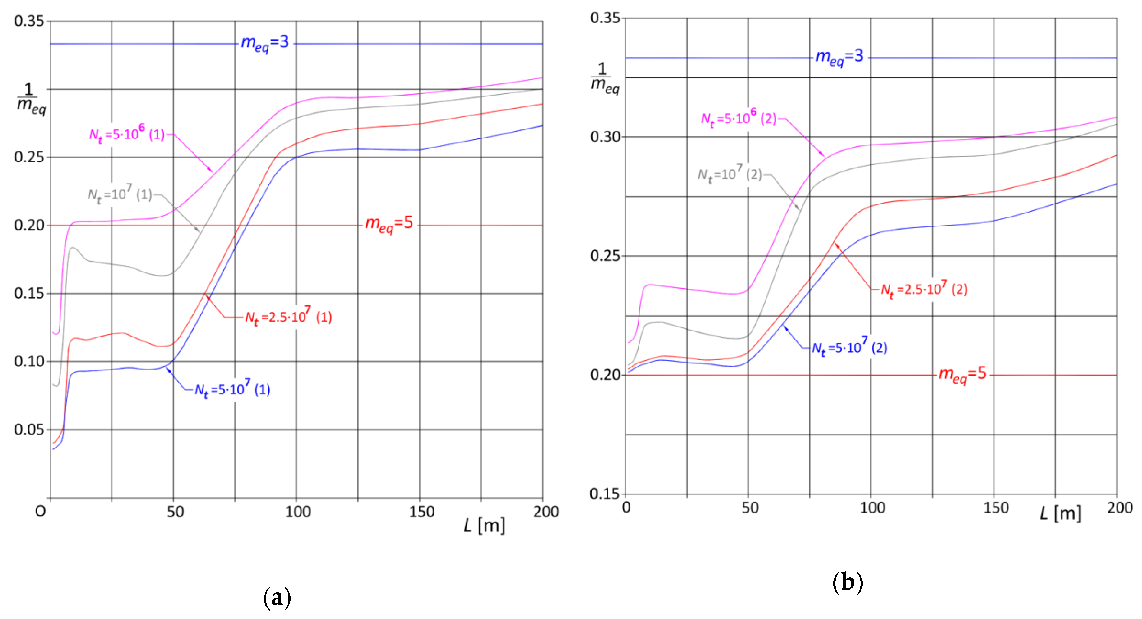
The damage equivalence factor curves, obtained applying Equation (25), are reported in Figure 13 and parameterized in terms of total flow, with, as said before, lorries being the reference flow. Curves in Figure 13a are produced referring to subcase 1, considering constant amplitude fatigue limit curves as per Figure 7a,b. Curves in Figure 13b are produced referring to subcase 2, considering details without constant amplitude fatigue limit, characterized by curves as per Figure 7c,d.
The analogous inverse of the equivalent slope curves are illustrated in Figure 14a,b.
To facilitate the interpretation of the curves, in these figures are also reported the horizontal lines corresponding to and to .
It must be pointed out that the results mainly depend on the traffic volume, for that reason they are absolutely general and can be easily extended to other static schemes and other kind of influence lines.
Investigation of the diagrams demonstrates that:
- as expected, increases as the traffic flow increases;
- independently on the shape of the curve, decreases as the span increases;
- for details characterized by constant amplitude fatigue limit, subcase 1, Figure 14a:
- ○
- in the interval , it results for lorries, for lorries, for lorries, and finally for lorries;
- ○
- when , it results for lorries, for lorries and for higher total flows;
- ○
- for , the curves approach these pertaining to details lacking a constant amplitude fatigue limit, which are discussed below.
- for details lacking a constant amplitude fatigue limit, subcase 2, Figure 14b:
- ○
- when , if lorries this results in , but reduces for smaller flows. More precisely, if lorries, it is for and for , while, if lorries, it is for and for ;
- ○
- when , this results in if lorries; if ; if lorries and, finally, if lorries.
These results underline that the equivalent slope depends on , on the shape of the curve and on the total traffic volume and that the assumption of a constant value for the slope could lead to erroneous, even on the unsafe side, estimates of the fatigue life.
Trivially, fatigue life determined assuming is overestimated when and or when and , underestimated otherwise. Moreover, errors are amplified when details characterized by constant amplitude fatigue limit are considered (subcase 1).
6. Conclusions
In consequence of the 96/53/EC Directive, some European countries allow the circulation on their respective road networks of Long and Heavy Vehicles, characterized by length and weight going beyond the limits imposed on common Heavy Good Vehicles.
The introduction of this kind of vehicles sprang from the twofold need to reduce transportation costs and pollutant emissions, but it could cause an increase of maintenance costs of existing infrastructure as well as of construction costs of new infrastructure.
Considering that traffic loads on road bridges provided in EN1991-2 were defined and calibrated using the traffic recorded in Auxerre, which is very severe, but does not include LHVs, their introduction could significantly impact not only the design of new bridges, but especially the assessment of the existing ones.
To discuss the consequence of circulation of Long and Heavy Vehicles on fatigue design of European bridges, the fatigue effects caused by the long-distance traffic recorded in the Netherlands (Moerdijk), characterized by a high percentage of LHVs, have been compared not only with the effects caused by Auxerre traffic but also with those produced by fatigue load models LM2 and LM4 of EN1991-2. To further corroborate the study, also actual Spanish traffic recorded in Igualada, near Barcelona, has been taken into account.
Assuming the same value for the global lorry flow, the fatigue effects induced by each traffic and each fatigue load model have been compared in terms of minimum fatigue categories needed to satisfy the fatigue verification or, equivalently, in terms of equivalence factors , in this latter case making specific reference to Auxerre traffic effects. To include most of the practical cases considered in the Eurocodes, details characterized by constant amplitude fatigue limit or not have been considered, adopting, case by case, the appropriate bilinear or trilinear characteristic curve.
The total flow on the slow lane during the fatigue life of the bridge has been usually assumed to be lorries, which is a typical value for motorways subject to intense traffic; but, for the sake of comparison, also lorries has been considered, representing main roads or secondary roads subject to low intensity commercial traffic.
Three important case studies have been analyzed, referring to influence lines of bending moments in simply supported and continuous beams, characterized by spans ranging in the interval .
Summarizing the considerations more extensively discussed in Section 4, it can be concluded that:
- Fatigue load models LM2 and LM4 adequately reproduce the Auxerre traffic effect, generally resulting on the safe side; but, in case of details characterized by constant amplitude fatigue limit, very small spans and intense lorry flows, fatigue load models LM2, which governs fatigue assessment, can lead to results slightly on the unsafe side.
- In the span range , where simultaneity effects are important, if consecutive lorries are hypothesized belonging both to the standardized set of fatigue load model LM4, the adoption of LM4 is very much on the safe side; in fact, the probability that weights of consecutive lorries are close to the equivalent values is not important; moreover in that range fatigue assessments are often not crucial. However, if necessary, it may be opportune to use real traffic data or artificially generated traffic.
- Auxerre traffic and, consequently, EN1991-2 load models cover not only Igualada traffic, but also LHV effects, as deduced from the Moerdijk traffic. Since the differences are particularly marked, this conclusion appears sound enough, even if it could require further investigations, taking into account other LHVs traffics.
- Axle load distribution of Moerdijk traffic is not particularly severe, probably because the LHVs are better controlled than HGVs, thus explaining why in some cases Igualada traffic is more aggressive than Moerdijk traffic.
- The fatigue load models for road bridges provided in the Eurocode EN1991-2 do not require major updates.
Finally, to complete the investigation, a special aspect of the damage-equivalence factor method has been investigated, concerning the influence of the total traffic volume on the fatigue damage. Actually, in the Eurocode approach, this aspect involves two damage-equivalence factors: , which considers traffic composition and annual lorry flow, and , which considers the fatigue design life of the bridge, nevertheless, since they both account for traffic volume, their product has been considered here to be the most relevant parameter.
The dependence of the damage-equivalence factor on , on the shape of the curve and on the total traffic volume has been critically discussed in Section 5, demonstrating that the adoption of simplified expressions for and , based on the assumption of a linear curve with constant conventional slope , could lead to erroneous estimates of the fatigue life that are even on the unsafe side. In fact, the equivalent slope can vary in a very wide range, especially when details characterized by constant amplitude fatigue limit are considered and the assessment is controlled by the unlimited fatigue life assessment, thus justifying improvements of the pertinent damage equivalence factors in the Eurocodes.
Obviously, the conclusions of the study are extremely general and apply also to artificially generated traffics, provided that their statistical parameters comply with those of the reference Auxerre traffic, or, more generally, with those of European traffics.
Further developments could be envisaged, mainly focusing on calibration of damage-equivalence factors.
Since the modern research field concerns the extension of the curves for steel details beyond the high-cycle fatigue range, in the very high fatigue domain, cycles, future studies could be addressed to deepen actual knowledge about this relevant topic, duly considering, on the one hand, that bridge details are generally in the “as welded” or “as laminated” condition and, on the other hand, that the stress cycles are characterized by variable amplitude.
Funding
This research received no external funding.
Acknowledgments
The author acknowledges Ane De Boer of the Directorate-General for Public Works and Water Management (Rijkswaterstaat) Centre for Infrastructure, Utrecht (NL), and Pilar Crespo Rodrigues of the Ministry of Development (Ministerio de Fomento), Madrid (ES), for sharing data.
Conflicts of Interest
The authors declare no conflict of interest.
Appendix A
| Symbols and Basic Nomenclature | |
| partial factor on fatigue actions; | |
| partial factor on fatigue resistance; | |
| basic stress range for damage equivalent factor method; | |
| fatigue category of the detail; | |
| detail category for which ; | |
| minimum detail category satisfying fatigue verifications; | |
| minimum detail category required by the Auxerre traffic; | |
| constant amplitude fatigue limit; | |
| detail category for which the Palmgren–Miner law provides unit fatigue damage ; | |
| stress range caused by fatigue load model LM3 of EN1991-2; | |
| cut-off limit; | |
| stress range in a cycle; | |
| maximum stress range relevant for fatigue assessment; | |
| additional amplification factor for fatigue verifications; | |
| damage-equivalence factor; | |
| single damage-equivalence factor ; | |
| damage-equivalence factor considering the effects of shape and length of the influence line; | |
| damage-equivalence factor considering the effects of the actual traffic in comparison with the Auxerre traffic; | |
| damage-equivalence factor considering the effects of the actual design working life; | |
| damage-equivalence factor considering the effects of multilane traffic; | |
| damage-equivalence factors; | |
| fatigue damage; | |
| reference fatigue damage caused by Auxerre traffic; | |
| fatigue damage caused by the actual traffic; | |
| equivalence factor ; | |
| , , | slopes of inclined branches of curves; |
| equivalent slope of the curve; | |
| abscissa of the knee point of a curve with two inclined branches; | |
| annual lorry flow of the Auxerre traffic; | |
| number of cycles in the stress spectrum at stress range; | |
| number of cycles to failure at ; | |
| annual flow of lorries weighing ; | |
| annual lorry flow; | |
| total lorry flow of the Auxerre traffic; | |
| total lorry flow; | |
| Q | single-axle load; |
| equivalent lorry weight; | |
| equivalent lorry weight of the Auxerre traffic ; | |
| tandem-axle load; | |
| total weights of lorry; | |
| tridem-axle load; | |
| curve | diagram giving the fatigue resistance as a function of number of cycles to failure in a constant amplitude fatigue test; |
| characteristic curve | characteristic curve: curve: curve corresponding to 5% probability of failure; : actual design working life; |
| equivalent uniformly distributed load of lorry; | |
Appendix B: Summary of the Procedure to Derive Equivalent Fatigue Categories
| The procedure to derive equivalent fatigue categories consists in the following steps: | |
| 1 | Assume an appropriate fatigue load model, represented by an appropriate conventional fatigue model or by a real traffic or by an artificially generated traffic; |
| 2 | Identify the number of occurrences of the given load model in the design working life of the bridge; |
| 3 | Identify the fatigue sensitive detail; |
| 4 | Identify the relevant shape of the curve, for example, considering if constant amplitude fatigue limit exists or not; |
| 5 | Identify the relevant influence surface for the fatigue effect considered; |
| 6 | Evaluate the stress history induced in the considered detail by the fatigue load model traveling the influence surface; |
| 7 | Determine, by means of a suitable cycle counting method (for example, the reservoir or the rainflow method), the stress spectrum; |
| 8 | Adopt the proper values of partial factors and ; |
| 9 | Magnify the stress spectrum multiplying each stress ranges by and ; |
| 10 | If fatigue limit does not exists go to step 15 |
| 11 | From the magnified stress spectrum (step 9), evaluate ; |
| 12 | ; |
| 13 | Determine from ; |
| 14 | Choose an “arbitrary” fatigue category of the detail; |
| 15 | Using the Palmgren–Miner formula, evaluate the fatigue damage induced by the magnified stress spectrum; |
| 16 | If change the fatigue category of the detail and go to step 14; |
| 17 | Set ; |
| 18 | If fatigue limit exists go to step 21 |
| 19 | Set |
| 20 | End the procedure; |
| 21 | Set ; |
| 22 | End the procedure. |
References
- EN1991-2 Eurocode 1: Actions on Structures—Part 2: Traffic Loads on Bridges; CEN: Brussels, Belgium, 2003.
- Bruls, A.; Croce, P.; Sanpaolesi, L.; Sedlacek, G. ENV 1991—Part 3: Traffic loads on bridges. Calibration of road load models for road bridges. In In Proceedings of the IABSE Colloquium Basis of Design and Actions on Structures; Background and Application of Eurocode 1, Delft, NL, 1996; IABSE Report, 74. IABSE: Zurich, Switzerland, 1996; pp. 439–454. [Google Scholar] [CrossRef]
- Croce, P.; Salvatore, W. Stochastic model for multilane traffic effects on bridges. J. Bridge Eng. 2001, 6, 136–143. [Google Scholar] [CrossRef]
- Jacob, B.; O’Brien, E.J.; Jehaes, S. (Eds.) Weigh-In-Motion of Road Vehicles; Final Report of COST 323 Action (WIM-LOAD); LCPC: Paris, France, 2002. [Google Scholar]
- O’Connor, A.J.; Jacob, B.; O’Brien, E.J.; Prat, M. Effects of traffic loads on road bridges—Preliminary studies for the re-assessment of the Eurocode 1, Part 3. In Proceedings of the 2nd European Conference on WIM of road vehicles, Lisbon, Portugal, 14–16 September 1998; pp. 231–242. [Google Scholar]
- Sedlacek, G.; Merzencih, G.; Paschen, M.; Bruls, A.; Sanapolesi, L.; Croce, P.; Calgaro, J.A.; Prat, M.; Jacob, B.; Leendertz, M.; et al. Background Document to EN1991—Part 2—Traffic Loads for Road Bridges and Consequences for the Design; JRC Scientific and Technical Reports; JRC: Ispra, Italy, 2008. [Google Scholar]
- Calgaro, J.A.; Tschumi, M.; Gulvanessian, H. Designer’s Guide to Eurocode 1: Actions on Bridges—EN 1991-2, EN 1991-1-1, -1-3 to -1-7 and EN 1990 ANNEX A2; Thomas Telford: London, UK, 2010. [Google Scholar]
- Directive 96/53/EC of 25 July 1996 Laying Down for Certain Road Vehicles Circulating Within the Community the Maximum Authorized Dimensions in National and International Traffic and the Maximum Authorized Weights in International Traffic, O.J. of European Union; European Union: Brussels, Belgium, 1996; Volume 235, pp. 59–75.
- OECD. Moving Freight with Better Trucks: Improving Safety, Productivity and Sustainability; OECD Publishing: Paris, France, 2011. [Google Scholar] [CrossRef]
- Aarts, L.; Honer, M.; Davydenko, I.; Quak, H.; de Bes van Staalduinen, J.; Verweij, K. Longer and Heavier Vehicles in The Netherlands: Facts, Figures and Experiences in the Period 1995–2010; Rijkswaterstaat Report; Directorate General for Public Works and Water Management: Utrecht, The Netherlands, 2010. [Google Scholar]
- Freundt, U.; Böning, S.; Kaschner, R. Road bridges between actual and future heavy load traffic—Road traffic loads according to DIN EN1991-2/NA. Beton Stahlbetonbau 2011, 11, 736–746. [Google Scholar] [CrossRef]
- Rymsza, J. Proposal to change the design load in the Eurocode 1 based on loads from vehicles with a mass of 60 tonnes. Transp. Res. Procedia 2016, 14, 4020–4029. [Google Scholar] [CrossRef] [Green Version]
- Lydon, M.; Taylor, S.E.; Robinson, D.; Mufti, A.; O’Brien, E.J. Recent developments in bridge weigh in motion (B-WIM). J. Civ. Struct. Health Monit. 2016, 6, 69–81. [Google Scholar] [CrossRef] [Green Version]
- Hellebrandt, L.; Blom, C.B.M.; Steenbergen, R.D.J.M. Probabilistic traffic load model for shortspan city bridges. Heron 2014, 59, 147–168. [Google Scholar]
- O’Brien, E.J.; Enright, B.; Getachew, A. Importance of the tail in truck weight modeling for bridge assessment. J. Bridge Eng. 2010, 15, 210–213. [Google Scholar] [CrossRef]
- O’Brien, E.J.; Enright, B. Modeling same-direction two-lane traffic for bridge loading. Struct. Saf. 2011, 33, 296–304. [Google Scholar] [CrossRef]
- Mohammed, O.; Gonzales, A.; Cantero, D. Dynamic impact of heavy long vehicles with equally spaced axles on short span highway bridges. Balt. J. Road Bridge Eng. 2018, 13, 1–13. [Google Scholar] [CrossRef] [Green Version]
- Jagelčáka, J.; Kiktováa, M.; Frančáka, M.; Marienka, P. The possibilities of using longer and heavier vehicle combinations in Slovakia. Transp. Res. Procedia 2019, 40, 271–278. [Google Scholar] [CrossRef]
- Chatzis, M.G.; Tirkkonen, T.; Lilja, H. Calibrating Eurocode’s fatigue load model 3 to specific national traffic composition. Struct. Eng. Int. 2012, 22, 232–237. [Google Scholar] [CrossRef]
- Maddah, N.; Nussbaumer, A. Analytical approach for improving damage equivalence factors. Eng. Struct. 2014, 59, 838–847. [Google Scholar] [CrossRef] [Green Version]
- Leander, J. Reliability evaluation of the Eurocode model for fatigue assessment of steel bridges. J. Constr. Steel. Res. 2018, 141, 1–8. [Google Scholar] [CrossRef]
- van Bentum, C.A.; Dijkstra, O.D. Process Description of Equivalent Fatigue Load on Bridge Decks; TNO Report 366 B UK; TNO: Delft, The Netherlands, 2008. [Google Scholar]
- EN1993-1-9 Eurocode 3: Design of Steel Structures—Part 1-9: Fatigue; CEN: Brussels, Belgium, 2005.
- EN1993-2 Eurocode 3: Design of Steel Structures—Part 2: Steel Bridges; CEN: Brussels, Belgium, 2006.
- EN1992-1-1 Eurocode 2: Design of Concrete Structures—Part 1-1: Concrete Bridges—General Rules and Rules for Buildings; CEN: Brussels, Belgium, 2004.
- EN1992-2 Eurocode 2: Design of Concrete Structures—Part 2: Concrete Bridges—Design and Detailing Rules; CEN: Brussels, Belgium, 2005.
- Jacob, B.; Cottineau, M.L. Weigh-in-motion for direct enforcement of overloaded commercial vehicles. Transp. Res. Procedia 2016, 14, 1413–1422. [Google Scholar] [CrossRef] [Green Version]
- Jacob, B.; Feypell-de La Beaumelle, V. Improving truck safety: Potential of weigh-in-motion technology. IATSS Res. 2010, 34, 9–15. [Google Scholar] [CrossRef] [Green Version]
- O’Connor, A.; O’Brien, E.J. Traffic load modeling and factors influencing the accuracy of predicted extremes. Can. J. Civ. Eng. 2005, 32, 270–278. [Google Scholar] [CrossRef] [Green Version]
- O’Brien, E.J.; Enright, B. Using Weigh-In-Motion data to determine aggressiveness of traffic for bridge loading. J. Bridge Eng. 2013, 18, 232–239. [Google Scholar] [CrossRef]
- Jacob, B.; Labry, D. Evaluation of the effects of heavy vehicles on bridge fatigue. In Proceedings of the 7th International Symposium on Heavy Vehicle Weights and Dimensions, Delft, The Netherlands, 16–20 June 2002; pp. 185–194. Available online: https://road-transport-technology.org/conferenceproceedings/2000s/ishvwd-7/ (accessed on 4 November 2019).
- Clemente, P.; De Stefano, A. (Eds.) WIM (Weigh in Motion), Load capacity and bridge performance. In Proceedings of Civil Structural Health Monitoring 2 Workshop, Taormina, IT, 2008; ENEA: Rome, Italy, 2010; Available online: https://www.enea.it/it/seguici/pubblicazioni/pdf-volumi/2010/v2010_03-proceedings_cshm2.pdf (accessed on 8 November 2019).
- Croce, P. Background to fatigue load models for Eurocode 1: Part 2 Traffic loads. Prog. Struct. Eng. Mater. 2001, 4, 250–263. [Google Scholar] [CrossRef]
- Croce, P. Improvement of damage equivalence λ-factors for railway steel bridges. In Proceedings of the 34th International Symposium on Bridge and Structural Engineering: Large Structures and Infrastructures for Environmentally Constrained and Urbanised Areas, Venice, Italy, 22–24 September 2010; IABSE: Zurich, Switzerland, 2010. [Google Scholar]
- Croce, P. Probabilistic models for vehicle interactions in fatigue assessment of bridges. Appl. Sci. 2019, 9, 5338. [Google Scholar] [CrossRef] [Green Version]
- McKay, M.D.; Beckman, R.J.; Conover, V.J. A comparison of three methods for selecting values of input variables in the analysis of output from a computer code. Technometrics 1979, 21, 239–245. [Google Scholar]
- Dowling, N.E. Fatigue failure predictions for complicated stress–strain histories. J. Mater. 1972, 2, 71–87. [Google Scholar]
- Dowling, S.D.; Socie, D.F. Simple rainflow counting algorithms. Int. J. Fatigue 1982, 7, 31–40. [Google Scholar] [CrossRef]
- Hong, N. A modified rainflow counting method. Int. J. Fatigue 1991, 13, 465–469. [Google Scholar] [CrossRef]
- ASM. ASM Handbook 19 Fatigue and Fracture; ASM International: Materials Park, OH, USA, 1996. [Google Scholar]
- Matsuishi, M.; Endo, T. Fatigue of metals subjected to varying stress. Jpn. Soc. Mech. Eng. 1968, 68, 37–40. [Google Scholar]
- Rychlik, I. A new definition of the rainflow cycle counting method. Int. J. Fatigue 1987, 9, 119–121. [Google Scholar] [CrossRef]
- Palmgren, A.G. Die Lebensdauer von Kugellagern. Z. Ver. Dtsch. Ing. 1924, 68, 339–341. (In German) [Google Scholar]
- Miner, M.A. Cumulative damage in fatigue. J. Appl. Mech. 1945, 12, 149–164. [Google Scholar]
Figure 1.
Lorry subclasses and symbols for Moerdijk traffic (adapted from [20]).
Figure 1.
Lorry subclasses and symbols for Moerdijk traffic (adapted from [20]).
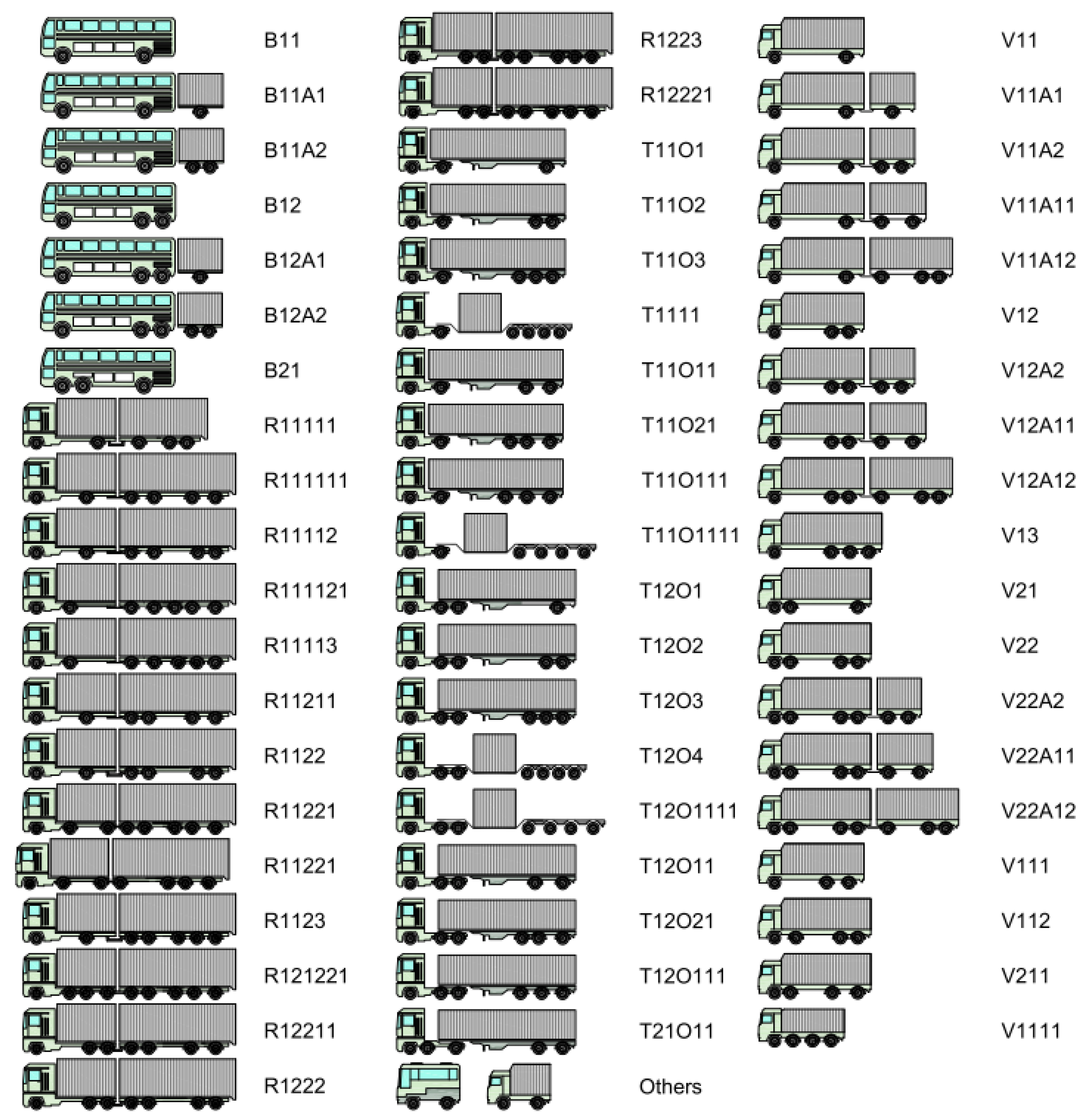
Figure 2.
Relative frequencies of traffic loads of Auxerre, Moerdijk and Igualada traffics: (a) single-axle load (); (b) tandem-axle load (; (c) tridem-axle load (); (d) total weight of lorry (); (e) equivalent uniformly distributed load () of lorry.
Figure 2.
Relative frequencies of traffic loads of Auxerre, Moerdijk and Igualada traffics: (a) single-axle load (); (b) tandem-axle load (; (c) tridem-axle load (); (d) total weight of lorry (); (e) equivalent uniformly distributed load () of lorry.
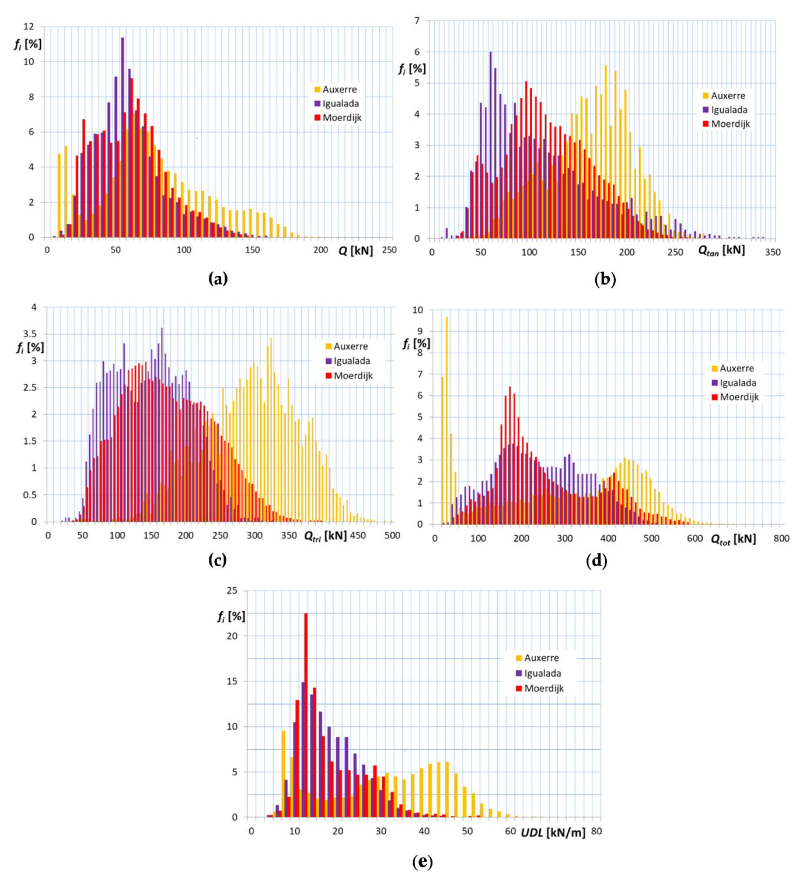


Figure 5.
Axle types for LM2 and LM4 standardized lorries—(dimensions are m, from [35]).
Figure 5.
Axle types for LM2 and LM4 standardized lorries—(dimensions are m, from [35]).
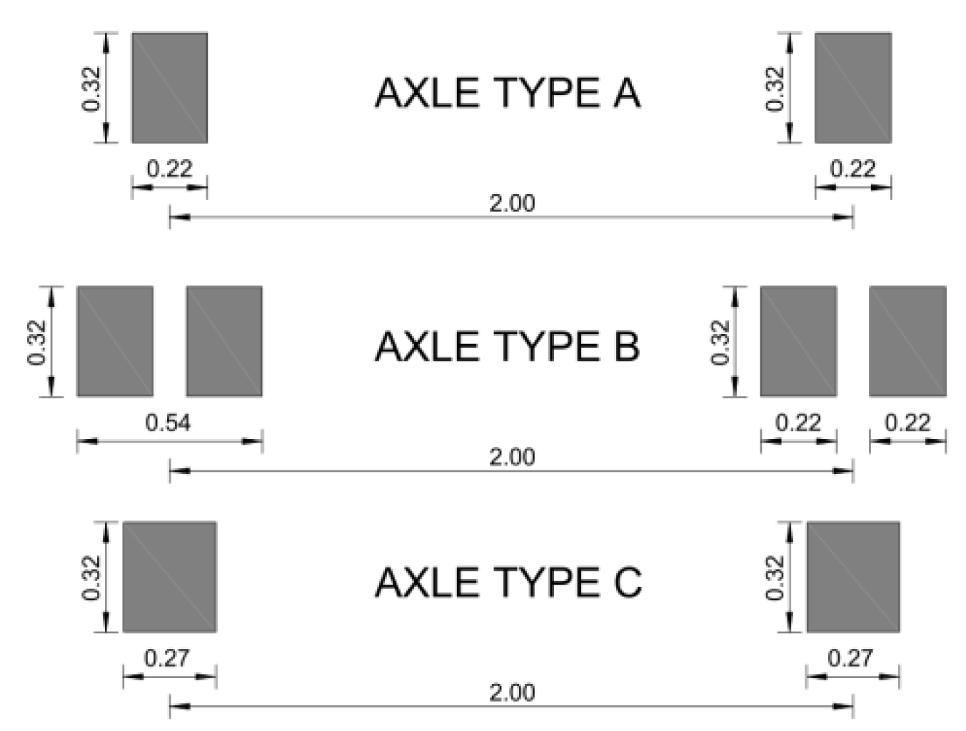
Figure 6.
Influence lines: (a) bending moment at midspan of a simply supported beam (case study no. 1); (b) hogging moment at intermediate support of a two-span continuous beam (case study no. 2); (c) bending moment at midspan of a three-span continuous beam (case study no. 3).
Figure 6.
Influence lines: (a) bending moment at midspan of a simply supported beam (case study no. 1); (b) hogging moment at intermediate support of a two-span continuous beam (case study no. 2); (c) bending moment at midspan of a three-span continuous beam (case study no. 3).
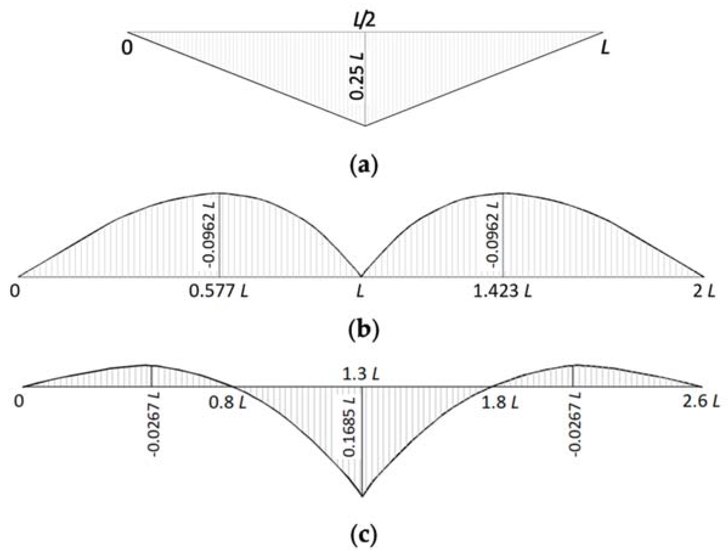
Figure 7.
Fatigue strength curves – Typical curves for most structural details (subcase 1): (a) bilinear; (b) trilinear—General bilinear curves (subcase 2): (c) all-purpose; (d) for some steel details.
Figure 7.
Fatigue strength curves – Typical curves for most structural details (subcase 1): (a) bilinear; (b) trilinear—General bilinear curves (subcase 2): (c) all-purpose; (d) for some steel details.
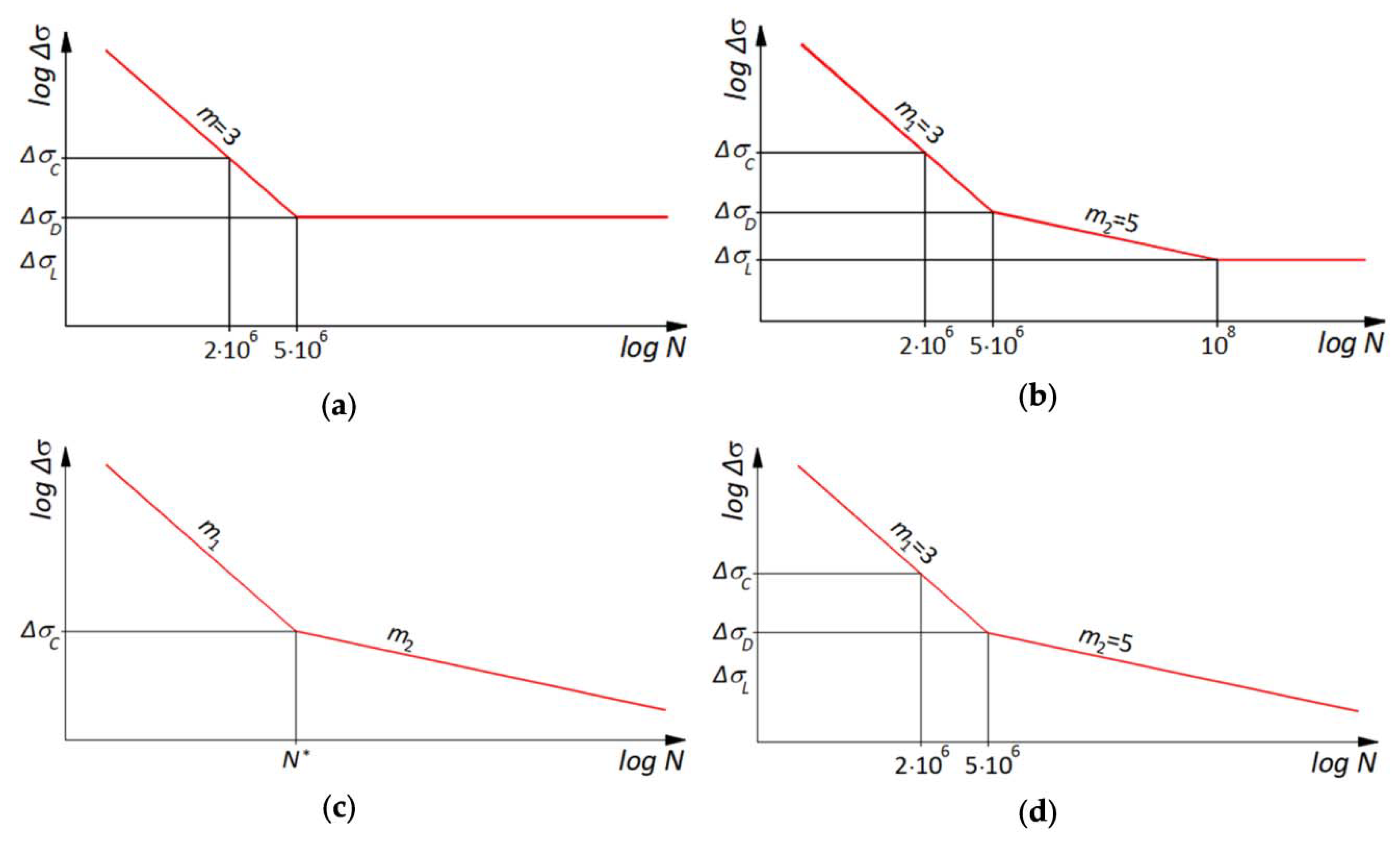
Figure 8.
Equivalence factor curves for bending moment at midspan of simply supported beams (case study no. 1—total lorry flow: lorries): (a) subcase 1— curves as per Figure 7a,b; (b) subcase 2— curves as per Figure 7c,d.
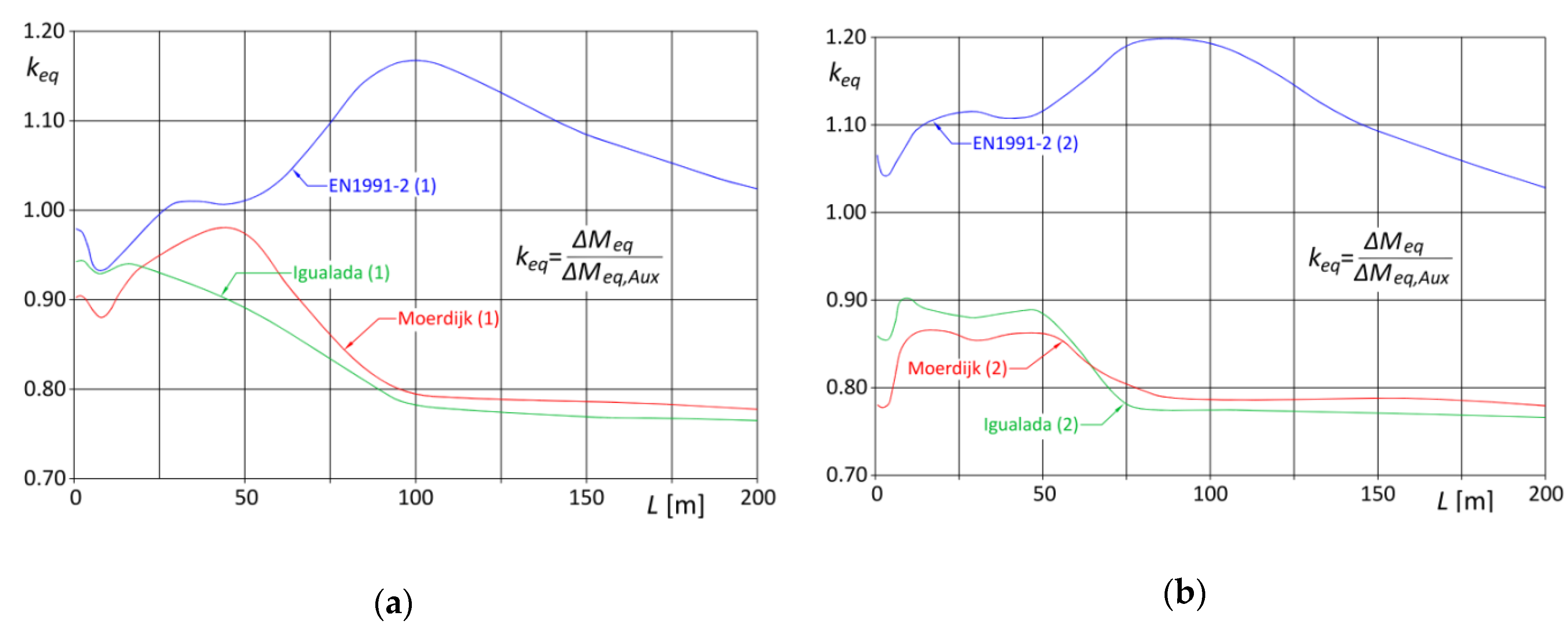
Figure 9.
Equivalence factor curves for hogging moment at intermediate support of two-span continuous beams (case study no. 2—total lorry flow: lorries): (a) subcase 1— curves as per Figure 7a,b; (b) subcase 2— curves as per Figure 7c,d.
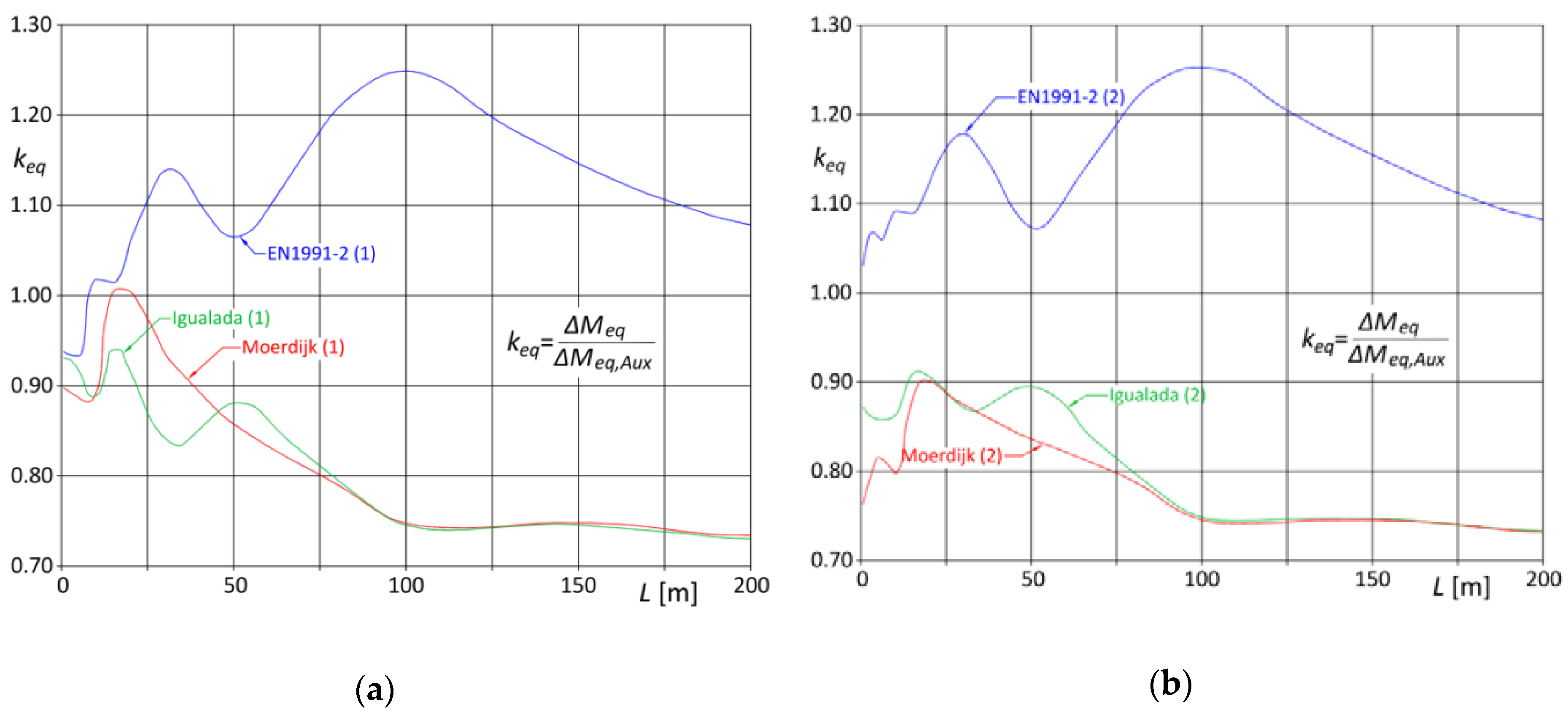
Figure 10.
Equivalence factor for bending moment at midspan of three-span continuous beams (case study no. 3—total lorry flow: lorries): (a) subcase 1— curves as per Figure 7a,b; (b) subcase 2— curves as per Figure 7c,d.
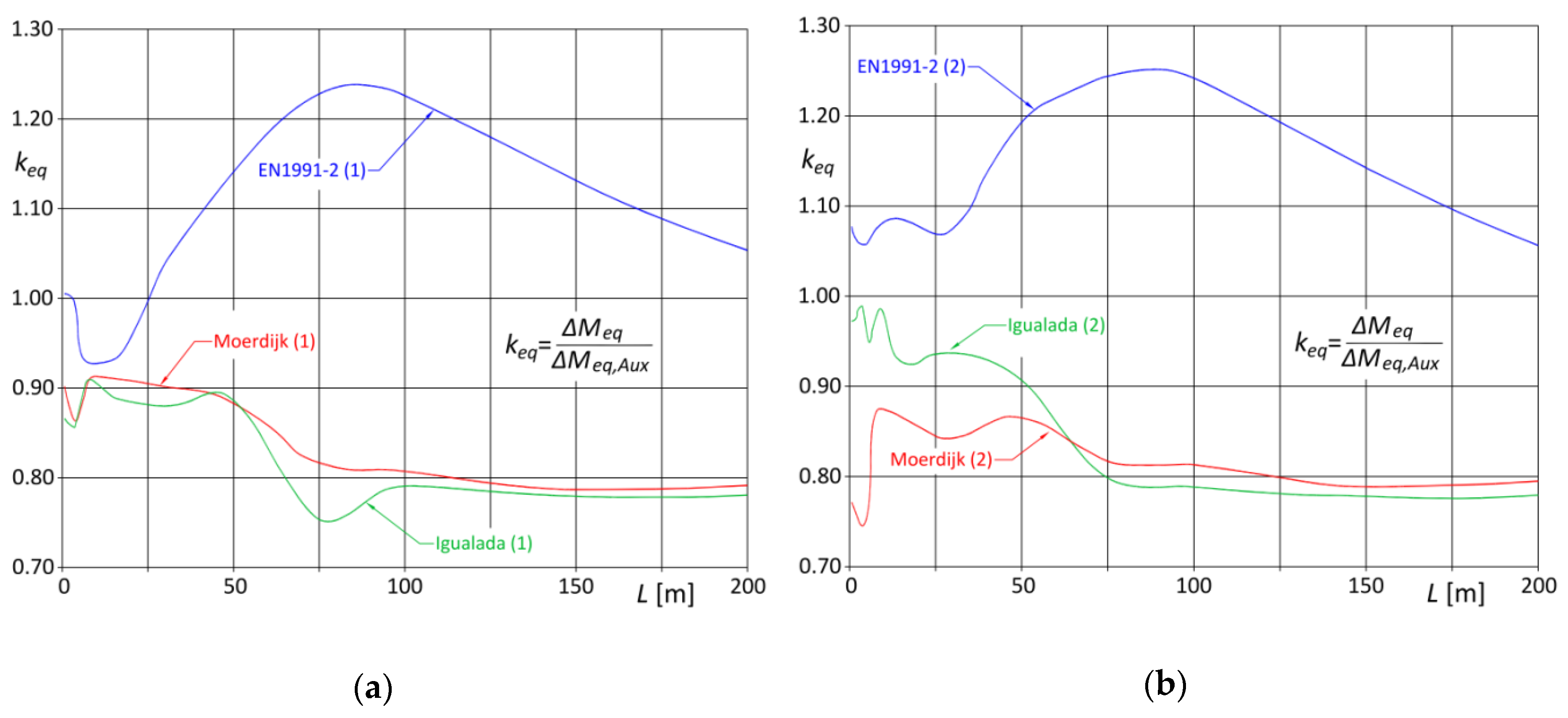
Figure 11.
Equivalence factor for bending moment at midspan of simply supported beams (case study no. 1—total lorry flow: lorries): (a) subcase 1— curves as per Figure 7a,b; (b) subcase 2— curves as per Figure 7c,d.
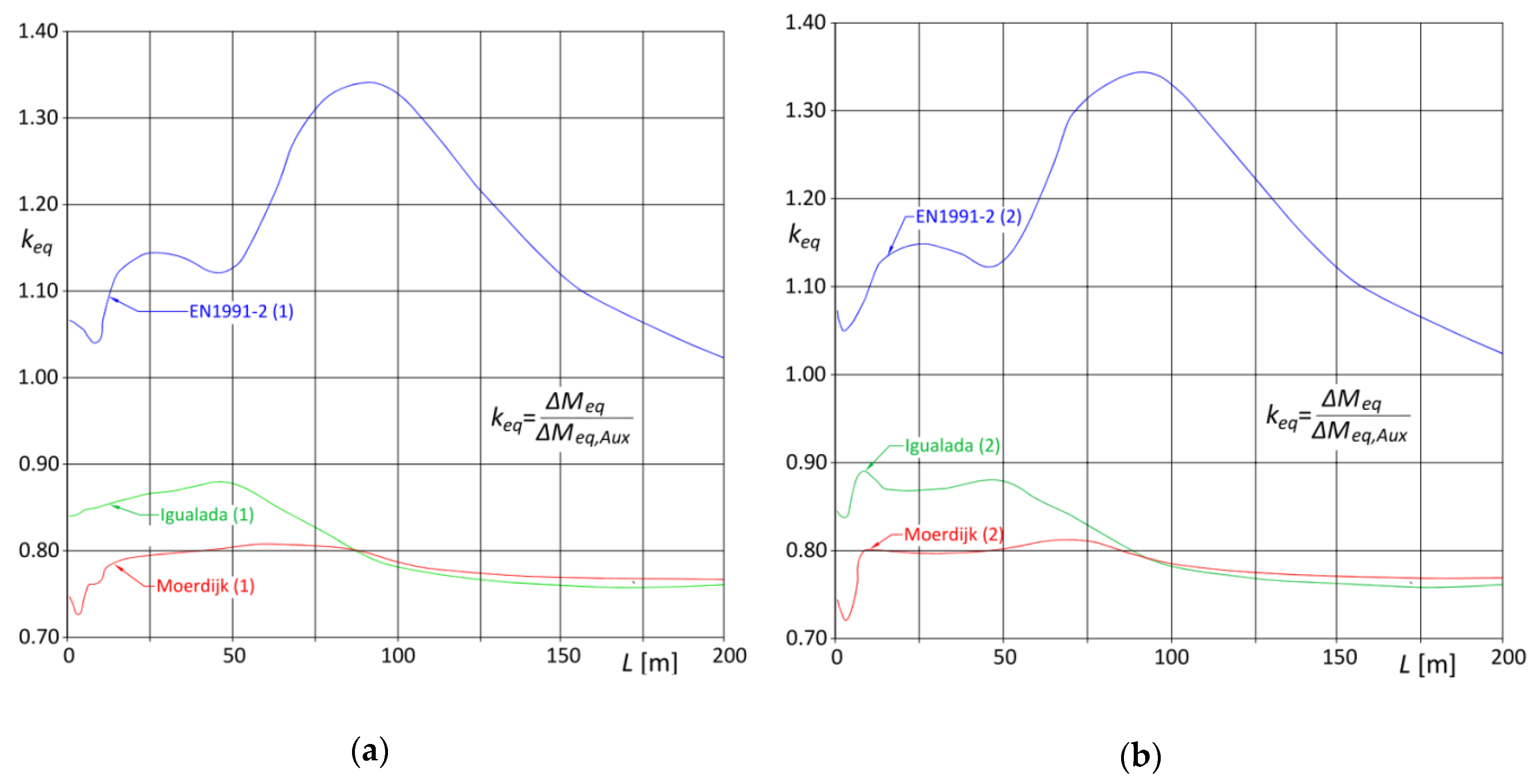

Figure 13.
Damage-equivalence factor curves for various total lorry flows for bending moment at midspan of simply supported beams (case study no. 1—reference flow: lorries): (a) subcase 1 — curves as per Figure 7a,b; (b) subcase 2— curves as per Figure 7c,d.
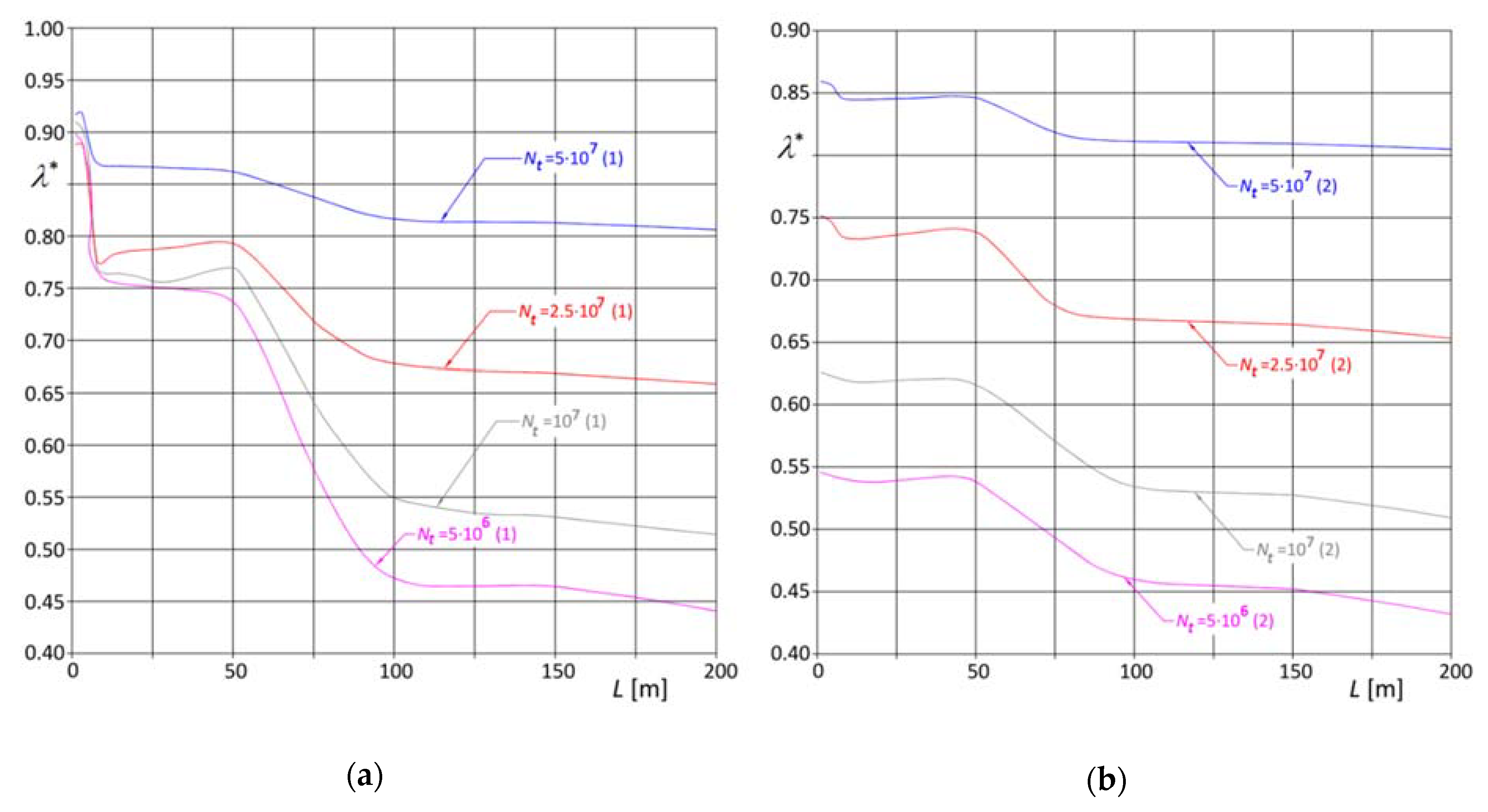
Figure 14.
Inverse of the equivalent slope curves for various total lorry flows for bending moment at midspan of simply supported beams (case study no. 1—reference flow: lorries): (a) subcase 1— curves as per Figure 7a,b; (b) subcase 2— curves as per Figure 7c,d.

Table 1.
Daily flow of single axles and statistical parameters of axle loads.
| Daily Flow | σ [kN] | |||
|---|---|---|---|---|
| Brohltal (DE) | 19,970 | 59.0 | 28.4 | 165.0 |
| Garonor (FR) 1982 | 8470 | 57.6 | 27.6 | 180.0 |
| Garonor (FR) 1984 | 11,593 | 59.3 | 30.0 | 195.0 |
| Auxerre (FR) (slow lane) | 10,442 | 82.5 | 35.2 | 195.0 |
| Auxerre (FR) (fast lane) | 581 | 73.1 | 41.2 | 200.0 |
| Fiano R. (IT) | ~15,000 | 56.8 | 32.9 | 192.01 |
| Piacenza (IT) | ~20,000 | 61.8 | 31.0 | 185.01 |
| Sasso Marconi (IT) | ~13,000 | 61.9 | 30.8 | 185.01 |
1 Extrapolated values.
Table 2.
Daily flow of lorries and statistical parameters of total loads.
| Daily Flow | σ [kN] | |||
|---|---|---|---|---|
| Brohltal (DE) | 4793 | 245.8 | 127.3 | 650.0 |
| Garonor (FR) 1982 | 2570 | 189.8 | 107.5 | 550.0 |
| Garonor (FR) 1984 | 3686 | 186.5 | 118.0 | 560.0 |
| Auxerre (FR) (slow lane) | 2630 | 326.7 | 144.9 | 630.0 |
| Auxerre (FR) (fast lane) | 153 | 277.2 | 163.6 | 670.0 |
| Fiano R. (IT) | ~4000 | 204.5 | 130.3 | 590.0 |
| Piacenza (IT) | ~5000 | 235.2 | 140.0 | 630.0 |
| Sasso Marconi (IT) | ~3500 | 224.9 | 149.0 | 620.0 |
Table 3.
Examples of physically incoherent measured data for 2-axle lorries (Moerdijk).
| Speed [m/s] | Inter-Axle [m] | Weight [kN] | Front Axle Load [kN] | Rear Axle Load [kN] |
|---|---|---|---|---|
| 30.6 | 21.02 | 707 | 398 | 309 |
| 3.3 | 13.05 | 613 | 208 | 405 |
| 3.3 | 62.02 | 684 | 318 | 366 |
| 27.2 | 11.32 | 689 | 353 | 336 |
© 2020 by the author. Licensee MDPI, Basel, Switzerland. This article is an open access article distributed under the terms and conditions of the Creative Commons Attribution (CC BY) license (http://creativecommons.org/licenses/by/4.0/).
Share and Cite
MDPI and ACS Style
Croce, P. Impact of Road Traffic Tendency in Europe on Fatigue Assessment of Bridges. Appl. Sci. 2020, 10, 1389. https://doi.org/10.3390/app10041389
AMA Style
Croce P. Impact of Road Traffic Tendency in Europe on Fatigue Assessment of Bridges. Applied Sciences. 2020; 10(4):1389. https://doi.org/10.3390/app10041389
Chicago/Turabian StyleCroce, Pietro. 2020. "Impact of Road Traffic Tendency in Europe on Fatigue Assessment of Bridges" Applied Sciences 10, no. 4: 1389. https://doi.org/10.3390/app10041389
Note that from the first issue of 2016, this journal uses article numbers instead of page numbers. See further details here.