Interval Identification of Thermal Parameters Using Trigonometric Series Surrogate Model and Unbiased Estimation Method

Featured Application

In this study, firstly, we proposed a novel modelling methodology for metal-foam materials in low porosity, which can simulate the actual geometry simply and closely. Moreover, to quantify the uncertainty of the metal-foam structure in the engineering heat transfer system, we proposed a novel multi-level optimization-based parameter identification method using a trigonometric series surrogate model and an unbiased estimation method. The proposed method provides an effective quantification for practical engineering problems, especially in the case without sufficientmeasurements.

Abstract

Metal-foam materials have been applied in many engineering fields in virtue of its high specific strength and desirable of thermodynamic properties. However, due to the inherent uncertainty of its attribute parameters, reliable analysis results are often ambiguous to obtain accurately. To overcome this drawback, this paper proposes a novel interval parameter identification method. Firstly, a novel modelling methodology is proposed to simulate the geometry of engineering metal foams. Subsequently, the concept of intervals is introduced to represent the uncertainty relationship between variables and responses in heat transfer systems. To improve computational efficiency, a novel augmented trigonometric series surrogate model is constructed. Moreover, unbiased estimation methods based on different probability distributions are presented to describe system measurement intervals. Then, a multi-level optimization-based identification strategy is proposed to seek the parameter interval efficiently. Eventually, an engineering heat transfer system is given to verify the feasibility of the proposed parameter identification method. This method can rapidly identify the unknown parameters of the system. The identification results demonstrate that this interval parameter identification method can quantify the uncertainty of a metal-foam structure in engineering heat transfer systems efficiently, especially for the actual case without sufficient measurements.

1. Introduction

In the past decades, metal-foam materials have attracted extensive attention due to its lightweight, high specific stiffness, favorable thermodynamic properties, and good energy absorption capacity, which are widely applied to various engineering fields, such as aeronautics, robotics, and biomedical engineering. However, as a typical porous material, the specific mechanical property can not be described accurately, which remains an issue for the research.

At present, the research on the structure of porous materials has made great achievements. Many researchers have attempted to predict the mechanical properties of this material through the structure of the periodic cells [1,2,3]. For instance, Gibson et al. [4] analyzed the physical mechanisms of the homogeneous deformation of the three-dimensional cellular foam structure. Demiray et al. [5] investigated the overall yield behavior of the three-dimensional model foam using the numerical homogenization method. Liu et al. [6] investigated the failure modes of the three-dimensional porous structure with the simplified model. Furthermore, with the improvement of X-ray technology, the method of a computerized tomography scan was adopted to research the internal microstructure in metal foams [7,8,9]. Ramirez et al. [10] looked at the elastoplastic deformation of open-cell foams with micro-CT, which showed better consistency agreement with experimental results. Islam et al. [11] simulated the dynamic deformation of closed-cell foams structure by using the technology of X-ray tomography. Sharma et al. [12] adopted CT scan technology to create a volume model and conducted corresponding experimental and numerical studies. Additionally, compared with periodic cells and CT scans, the Voronoi method was widely used to describe the random and complex mesostructure of the porous material factually [13,14,15]. Zhang et al. [16] used the Voronoi method to construct the model of the open aluminum foam material and performed the study of a hypervelocity impact. In the research of Zhang et al. [17], various numerical simulations were carried out to study the mechanical properties of Voronoi models. Moreover, Skibinski et al. [18] modeled the porous structure with the Laguerre–Voronoi Tessellations method and researched the influence of various geometric parameters on the effective thermal conductivity.

However, although the periodic unit cells approach is relatively accurate in describing the dependence of a single cell transformation characteristic on porosity, actual mechanical properties are not well known when the complex and stochastic morphology was considered. Meanwhile, the CT scan technology requires enormous computational resources and computational time to achieve satisfactory results, which is not realistic for extensive engineering calculations. Besides, for the method of Voronoi tessellation, plenty of previous studies have adopted it to describe the stochastic characteristics of the real metal-foam structure. Nevertheless, most of the implementation algorithms require a large amount of computation and ignore the randomness of the wall thickness [19,20,21]. Additionally, as a polycrystalline structure composed of an enormous number of cells, its properties are not determined by the feature of a single cell but by the connectivity and interaction between cells. Hence, the mechanical properties are often uncertain, coupled with the complicated external factors, uncertainties inevitably exist in the heat transfer system of the metal-foam structure.

For the practical engineering system, the process of parameter identification is considered to be more necessary to quantify these uncertainties, which has been extensively researched [22,23,24,25]. These methods are mainly divided into two types: probabilistic and non-probabilistic. For the method of probabilistic, Furukawa et al. [26] proposed a methodology to identify defects based on the theory of random probability. Wan et al. [27] adopted the Bayesian approach coupled with the Gaussian process model to quantify the uncertainty parameter in the stochastic problem. In the research of Wang et al. [28], a novel identification method for a steady-state heat transfer problem based on fuzzy uncertainty was presented. To the present, probabilistic-based parameter identification methods have been researched widely. However, a serious problem needs to be noticed, that is, the premise of applying these methods is that the probability distribution function is known, which is difficult to obtain accurately for the practical engineering systems.

In recent years, the non-probabilistic method based on interval theory has been proposed to describe the uncertainty [29,30,31,32], which avoids the calculation of the probability density function and only needs the lower bound (LB) and upper bound (UB) of the sample interval. Khodaparast et al. [33] presented a novel parameter identification method for structure system with the technology of sensitivity analysis of the Kriging meta-model. To avoid the effects of interval expansion, Fang et al. [34] put forward an improved parameter identification method by modifying the response surface model. Guo et al. [35,36] studied polynomial response surface and Radial Basis Function neural networks model, respectively, and proposed a novel interval parameter identification strategy. Besides, Wang et al. [37] constructed an interval identification method for heat transfer problems based on the nested-loop strategy and chaos expansion. In the research of Wang et al. [38], an augmented Fourier polynomial surrogate model was proposed and applied to the parameter identification of structural systems with novel optimization strategy. Although the method based on interval theory has received extensive attention and research, some issues remain. For instance, the computational cost of the system’s original implicit-based model is immeasurable in practical engineering systems which require a simple and efficient surrogate model. In addition, most of the identification strategies adopted in the above study are too complicated and cannot be effectively applied to the interval problem well. Additionally, for the evaluation of measurement intervals, the traditional extremum method may cause these intervals biased.

Hence, firstly, this paper presents a novel modelling methodology based on the Voronoi tessellation to simulate the geometry concisely and factually for low porosity metal-foam materials. Additionally, for the uncertainty of parameters in the heat transfer problem, an improved interval theory-based parameter identification strategy is designed, which adopts the novel augmented trigonometric series polynomial model (ATP) and an unbiased interval estimation method. Eventually, an engineering heat transfer system is provided to verify the feasibility of the proposed method.

2. Model Structures

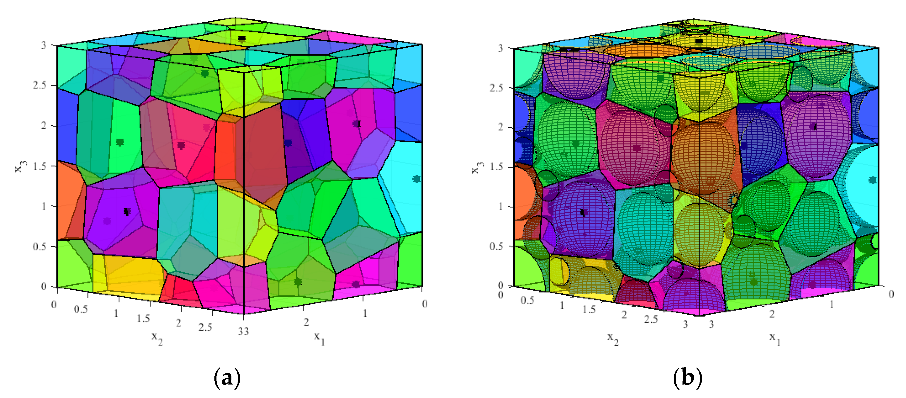
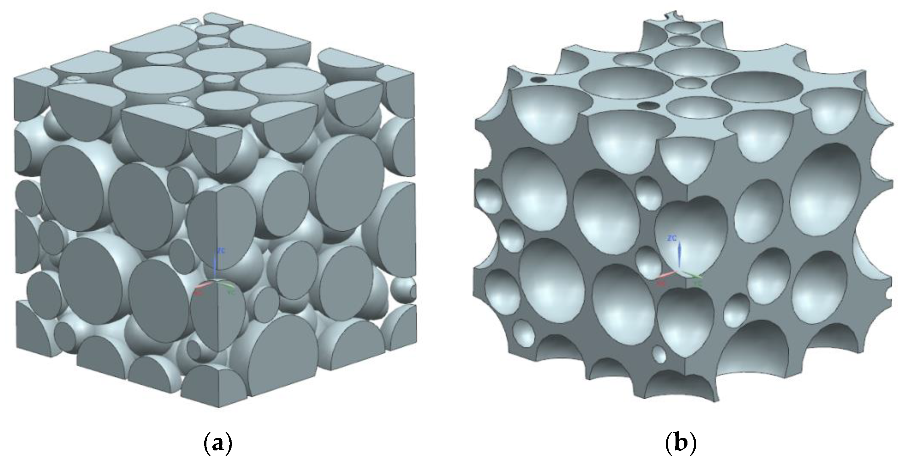
2.1. Generation of a Closed-Cell Foam Structure

To simulate the realistic pore geometry effectively, a novel Voronoi-based modelling methodology was described hereinafter for the closed-cell metal-foam materials with low porosity. The Voronoi tessellation is a finite partition method that divides a space into n independent regions with n separate nucleation points. If $\mathit{P}=\{{\mathit{p}}_1,{\mathit{p}}_2,\cdot \cdot \cdot ,{\mathit{p}}_n\}$ is a set of n nucleation points in space ${\mathit{X}}^m$, the Voronoi region ${\mathit{R}}_{\mathit{i}}$ can be defined as

$${\mathit{R}}_{\mathit{i}}=\{x\in \mathit{X}|d(x,{\mathit{p}}_{\mathit{i}})\le d(x,{\mathit{p}}_{\mathit{j}})for\text{\hspace{0.17em}}allj\ne i\}$$

(1)

where $d(\cdot ,\cdot )$ denotes the normal Euclidean distance. For each nucleation point, there is a corresponding region consisting of a specific subset, which satisfies that all the points in the subset are closer to that nucleation point than to any other.

The metal-foam model can be created in the following steps, randomly generate nucleation points, Voronoi tessellation, spheres packing, randomly define boundary thickness, and generate metal-foam model.

The first is the random generation of nucleation points, which largely determines the location and size of the pores. Here, the perturbation nucleation point method is adopted to describe the randomness of the pores. The specific expressions are as follows.

$$\begin{array}{l}{x}_i=x_{oi}+norm(0,k)\\ y_i=y_{oi}+norm(0,k),i=1,2,...,n\\ z_i=z_{oi}+norm(0,k)\end{array}$$

(2)

where $\{\mathit{x},\mathit{y},\mathit{z}\}$ are the location of nucleation points, and the set of $\{{\mathit{x}}_{\mathit{o}},{\mathit{y}}_{\mathit{o}},{\mathit{z}}_{\mathit{o}}\}$ are the original points that uniformly distributed. The symbol of $norm(0,k)$ denotes a Gaussian random distribution with a mean of 0 and a standard deviation of k, where the value of $k$ determines the perturbation degree of the new nucleation points distribution.

Subsequently, the Voronoi tessellation method is applied to divide a cube space into multiple convex polyhedra with the random nucleation points generated above. The number of polyhedra depends on the number of these nucleation points.

Then, to create the closed-cell pore structure, the algorithm of spheres random packing is proposed. The algorithm starts with searching for a maximum volume sphere in each convex polyhedron and randomly defines the distance between the spheres. If the volume of these spheres does not meet the pre-set porosity requirements, the procedure will continue the search of maximum volume spheres in the remaining space one by one, until the requirements are met. Moreover, the randomness of the boundary thickness between pores is taken into account in the searching process of spheres. Meanwhile, for convex polyhedra on boundary surfaces, the boundary constraint is removed to search the larger part of the sphere to simulate the characteristics of the surface pores.

Eventually, the Boolean operation is employed to subtract the resulting three-dimensional (3D) solid pores from the solid cube. Thus, the metal foam structure can be created effectively, which consists of multiple random pores.

In the proposed approach, the Voronoi structure and the packed spheres were generated in MATLAB (R2016b, MathWorks, USA) by utilizing the algorithm described above. Then, the 3D metal-foam solid model was created in UG software with the automation procedure, which was developed based on the C/C++ language and UG secondary development technology. The basic steps of constructing the 3D metal-foam model are presented in Figure 1 and Figure 2, which can provide a simple and effective method for practical engineering.

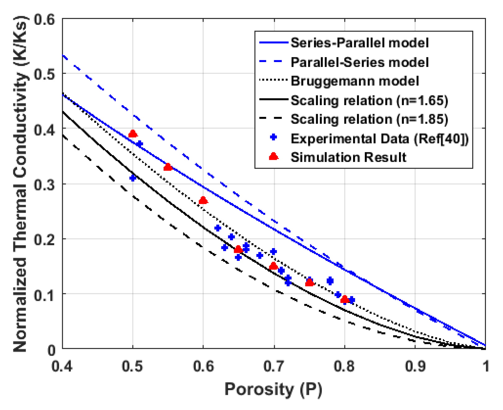
2.2. Effective Thermal Conductivity of the Foam Structure

Similar to the definition of the solid material conductivity, a steady-state heat transfer equation of metal-foam materials can be conducted. Hence, the thermal conductivity of metal-foam materials can be defined as

$$K_f=\frac{q}{\Delta T/H}$$

(3)

where $q$ is the heat flux, $\Delta T$ represents the temperature difference of the measured surface, and $H$ denotes the thickness of the sample.

In order to predict the thermal conductivity of closed-cell metal-foams, a wide variety of theoretical modes have been developed [39,40,41]. For instance, the simplest models, the Series-Parallel and the Parallel-Series models were constructed with the assumption of a cubical geometry. For particles of various shapes, the Bruggemann model was presented for this particular case. Moreover, the empirical model of scaling relation was proposed for metal-foams with a fitting parameter.

Series-Parallel model:

$${K=K}_s(1-P^{2/3})+\frac{K_s\cdot P^{2/3}}{K_{\mathrm{a}}+(K_s-K_{\mathrm{a}})P^{1/3}}$$

(4)

Parallel-Series model:

$${K=K}_s\cdot \frac{K_s-(K_s-K_{\mathrm{a}})P^{2/3}}{K_s-(K_s-K_{\mathrm{a}})(P^{2/3}-P)}$$

(5)

Bruggemann model:

$$1-P=\left(\frac{K_{\mathrm{a}}-K}{K_{\mathrm{a}}-K_s}\right)\cdot {\left(\frac{K_s}{K}\right)}^{1/3}$$

(6)

Scaling relation model:

$$K=K_s\cdot {(1-P)}^{\mathrm{n}},n\in [1.65,1.85]$$

(7)

where $K$ is the overall conductivity of the metal-foam, $K_s$ and $K_{\mathrm{a}}$ stand for the conductivity of the metal and air, respectively, and $P$ denotes the porosity of the foam.

Apart from the above theoretical prediction models, E. Solórzano [40] gave the experimental data of the thermal conductivity of closed-cell AlSi7 foams with porosities between 0.5 and 0.8, which was shown in Figure 3.

The MSC.Patran is employed to investigate the thermal conductivity of closed-cell metal-foam obtained by the methodology in Section 2.1. The conductivity of metal and air is 167 W/(m·K) and 0.025 W/(m·K), respectively. The Figure 3 shows the mismatch between the simulation result and the experimental data and the predicted value of models. Evidently, the simulation result showed good agreement with thermal conductivity values obtained by the literature and the prediction model. Furthermore, according to the growth of porosity, the thermal conductivity of metal-foam decreases, which further demonstrates the proposed modelling methodology of metal-foam structure can simulate the realistic pore geometry effectively, especially for the property of thermodynamic.

3. Theory Preparation

3.1. Thermodynamics Computational Model with Uncertainty

The governing equation of steady-state thermal analysis varies with the type of heat transfer systems. Without loss of generality, the general heat equilibrium equation can be expressed as:

$$[\mathit{K}]\left\{\mathit{T}\right\}=\left\{\mathit{Q}\right\}$$

(8)

where $\mathit{K}$ is the heat stiffiness matrix, $\mathit{T}$ stands for the system temperature response vector, and $\mathit{Q}$ denotes the heat flow vector.

In practical engineering, the uncertainty of the heat transfer system in terms of material properties, geometric properties, and modeling conditions is inevitable due to the complex external factors and inadequate cognition. Generally, these uncertainty parameters are usually represented in terms of a fluctuation value $\Delta x$ and a nominal value $x^0$:

$$\begin{gathered} {\mathit{X}}_i=[\underset{\_}{x_i},\overline{x_i}]=x_i{}^0+\Delta x_i \\ {\mathit{X}}^I=[\underset{\_}{\mathit{X}},\overline{\mathit{X}}]=\left\{\left(x_1,\cdot \cdot \cdot ,x_n\right)\in R^n|x_i\in X_i,i=1,\cdot \cdot \cdot ,n\right\} \end{gathered}$$

(9)

where $\underset{\_}{x_i}$ and $\overline{x_i}$ describe the bound of interval variable ${\mathit{X}}_i$, and $\underset{\_}{\mathit{X}}$ and $\overline{\mathit{X}}$ denote the LB and UB vector of ${\mathit{X}}^I$, respectively.

By introducing uncertainty parameters ${\mathit{X}}^I$, the general heat equilibrium equation in Equation (8) can be redefined as

$$[\mathit{K}({\mathit{X}}^I)]\{\mathit{T}({\mathit{X}}^I)\}=\{\mathit{Q}({\mathit{X}}^I)\}$$

(10)

Generally, due to the interval vector ${\mathit{X}}^I$, the value of system responses would varies within a certain range. Theoretically speaking, the system temperature vector can be calculated as

$$\underset{\_}{\mathit{T}}=\underset{\underset{\_}{\mathit{X}}\le \mathit{X}\le \overline{\mathit{X}}}{\min }\left\{\mathit{T}\left({\mathit{X}}^{\mathit{I}}\right)\left|\mathit{K}\right({\mathit{X}}^{\mathit{I}}\left)\mathit{T}\right({\mathit{X}}^{\mathit{I}}\left)=\mathit{Q}\right({\mathit{X}}^{\mathit{I}})\right\}$$

(11)

$$\overline{\mathit{T}}=\underset{\underset{\_}{\mathit{X}}\le \mathit{X}\le \overline{\mathit{X}}}{\max }\left\{\mathit{T}\left({\mathit{X}}^{\mathit{I}}\right)\left|\mathit{K}\right({\mathit{X}}^{\mathit{I}}\left)\mathit{T}\right({\mathit{X}}^{\mathit{I}}\left)=\mathit{Q}\right({\mathit{X}}^{\mathit{I}})\right\}$$

(12)

3.2. Augmented Trigonometric Polynomial Surrogate Model

Compared with the explicit mathematical model, in practical terms, the optimization process of engineering systems often has ambiguous physical relationships and considerable computational cost. To improve the computational efficiency and accuracy, the ATP surrogate model was proposed in this section.

If a periodical function $f\left(x\right)$ changes within $\left[-\pi ,\pi \right]$, there exists a Fourier series $P\left(x\right)$ converging to $f\left(x\right)$, which can be expressed as

$${\Vert f\left(x\right)-P\left(x\right)\Vert }_{\infty }<\epsilon \begin{array}{cc},& x\in \left[-\pi ,\pi \right]\end{array}$$

(13)

Then, the function $f\left(x\right)$ can be approximated by $P\left(x\right)$ with the combined forms of cosine and sine functions.

$$f\left(x\right)\approx P\left(x\right)=\frac{a_0}{2}+{\displaystyle \sum _{i=1}^n\left(a_i\cos ix+b_i\sin ix\right)}$$

(14)

Theoretically, by solving the above trigonometric coefficients, we can obtain the Fourier approximation of $f\left(x\right)$. However, for a multi-dimensional problem, the sharp increase in the number of trigonometric coefficients is a great challenge to the entire calculation process.

To simplify the approximation expression [42], we adopt the cosine as the basis function. Therefore, the function $f\left(x\right)$ can be expressed with the cosine function.

$$f\left(x\right)\approx P_{cos}\left(x\right)=\frac{a_0}{2}+{\displaystyle \sum _{i=1}^n{a}_i\cos ix},x\in [0,\pi ]$$

(15)

Without losing generality, for an s-dimensional continuous function $f\left(x_1,\cdot \cdot \cdot ,x_s\right)$, the approximation $P_{\cos }\left(x_1,\cdot \cdot \cdot ,x_s\right)$ can be expressed as the form of tensor product.

$$\begin{array}{l}f\left(x_1,\cdot \cdot \cdot ,x_s\right)\approx P_{\cos }\left(x_1,\cdot \cdot \cdot ,x_s\right)\\ =P_{\cos }\left({\theta }_1,\cdot \cdot \cdot ,{\theta }_s\right)\\ ={{\displaystyle \sum _{i_1=0}^{2n_1}\cdot \cdot \cdot {\displaystyle \sum _{i_s=0}^{2n_s}\left(\frac{1}{2}\right)}}}^s{g}_{i_1,\cdot \cdot \cdot ,}{}_{i_s}{C}_{i_1,\cdot \cdot \cdot ,}{}_{i_s}\left({\theta }_1,\cdot \cdot \cdot ,{\theta }_s\right)\end{array}$$

(16)

where $C_{i_1,\cdot \cdot \cdot ,}{}_{i_s}\left({\theta }_1,\cdot \cdot \cdot ,{\theta }_s\right)$ is the basis function of the s-dimensional system, $g_{i_1,\cdot \cdot \cdot ,}{}_{i_s}$ is the corresponding expansion coefficient.

Here, we have compared the approximation accuracy of cosine-based, sine-based, and combined-based with the same example, where the maximum relative error $err{o}_{\max }$ is used to judge the approximation effect numerically.

Example: $f\left(x\right)=2+\arctan x$, where $x\in [-1,1]$.

$$err{o}_{\max }=\max \left|\frac{f^a-f}{f}\right|\times 100$$

(17)

Note from Figure 4, the approximation of cosine-based basis function shows better performance than others with higher precision and fewer coefficients. However, for the weak nonlinear problem, we can see that the approximation effect of this function is not perfect even if the order is 5. Therefore, we added a polynomial term to the cosine-based basis function to augment its approximation performance.

Thus, the augmented cosine series-based surrogate model can be constructed, as follows.

$$f\left(\mathit{x}\right)\approx {{\displaystyle \sum _{i_1=0}^{n_1}\cdot \cdot \cdot {\displaystyle \sum _{i_s=0}^{n_s}\left(\frac{1}{2}\right)}}}^s{g}_{i_1,\cdot \cdot \cdot ,}{}_{i_s}{C}_{i_1,\cdot \cdot \cdot ,}{}_{i_s}\left(\mathit{x}\right)+{\displaystyle \sum _{j=1}^m{h}_j{k}_j\left(\mathit{x}\right)}={\mathit{\beta }}^T\mathit{\alpha }+{\mathit{h}}^T\mathit{k}$$

(18)

where

$$\mathit{\beta }={\left[{\beta }_1,\cdot \cdot \cdot ,{\beta }_m\right]}^T={\left(1/2\right)}^s{[g_{0,\cdot \cdot \cdot ,}{}_0,\cdot \cdot \cdot ,g_{i_1,\cdot \cdot \cdot ,}{}_{i_s},\cdot \cdot \cdot ,g_{2n_1,\cdot \cdot \cdot ,}{}_{2n_s}]}^T$$

(19)

$$\mathit{\alpha }={\left[{\alpha }_1,\cdot \cdot \cdot ,{\alpha }_m\right]}^T={[C_{0,\cdot \cdot \cdot ,}{}_0\left(\mathit{x}\right),\cdot \cdot \cdot ,C_{i_1,\cdot \cdot \cdot ,}{}_{i_s}\left(\mathit{x}\right),\cdot \cdot \cdot ,C_{n_1,\cdot \cdot \cdot ,}{}_{n_s}\left(\mathit{x}\right)]}^T$$

(20)

It should be pointed out that the polynomial term of $k\left(\mathit{x}\right)$ can be extended in different forms according to actual needs. For instance, $\mathit{x}$, ${\mathit{x}}^2$, ${\mathit{x}}^3$, among others. In our work, the first order item was adopted to augment the approximation ability of the cosine series-based surrogate model.

Correspondingly, a group of equations with unknown coefficients can be derived.

$$\left[\begin{array}{ccccccc}{\alpha }_1\left({\mathit{x}}_1\right)& \cdots & {\alpha }_n\left({\mathit{x}}_1\right)& ┆& k_1\left({\mathit{x}}_1\right)& \cdots & k_m\left({\mathit{x}}_1\right)\\ ⋮& \ddots & ⋮& ┆& ⋮& \ddots & ⋮\\ {\alpha }_1\left({\mathit{x}}_p\right)& \cdots & {\alpha }_n\left({\mathit{x}}_p\right)& ┆& k_1\left({\mathit{x}}_p\right)& \cdots & k_m\left({\mathit{x}}_p\right)\end{array}\right]\left\{\begin{array}{c}\mathit{\beta }\\ \mathit{h}\end{array}\right\}=\left[\begin{array}{c}f\left({\mathit{x}}_1\right)\\ ⋮\\ f\left({\mathit{x}}_p\right)\end{array}\right]$$

(21)

The ATP surrogate model is a polynomial regression method, which is composed of cosine-based trigonometric series and augmented polynomial term. The novel ATP surrogate model can be applied to the optimization process of engineering systems with uncertainty.

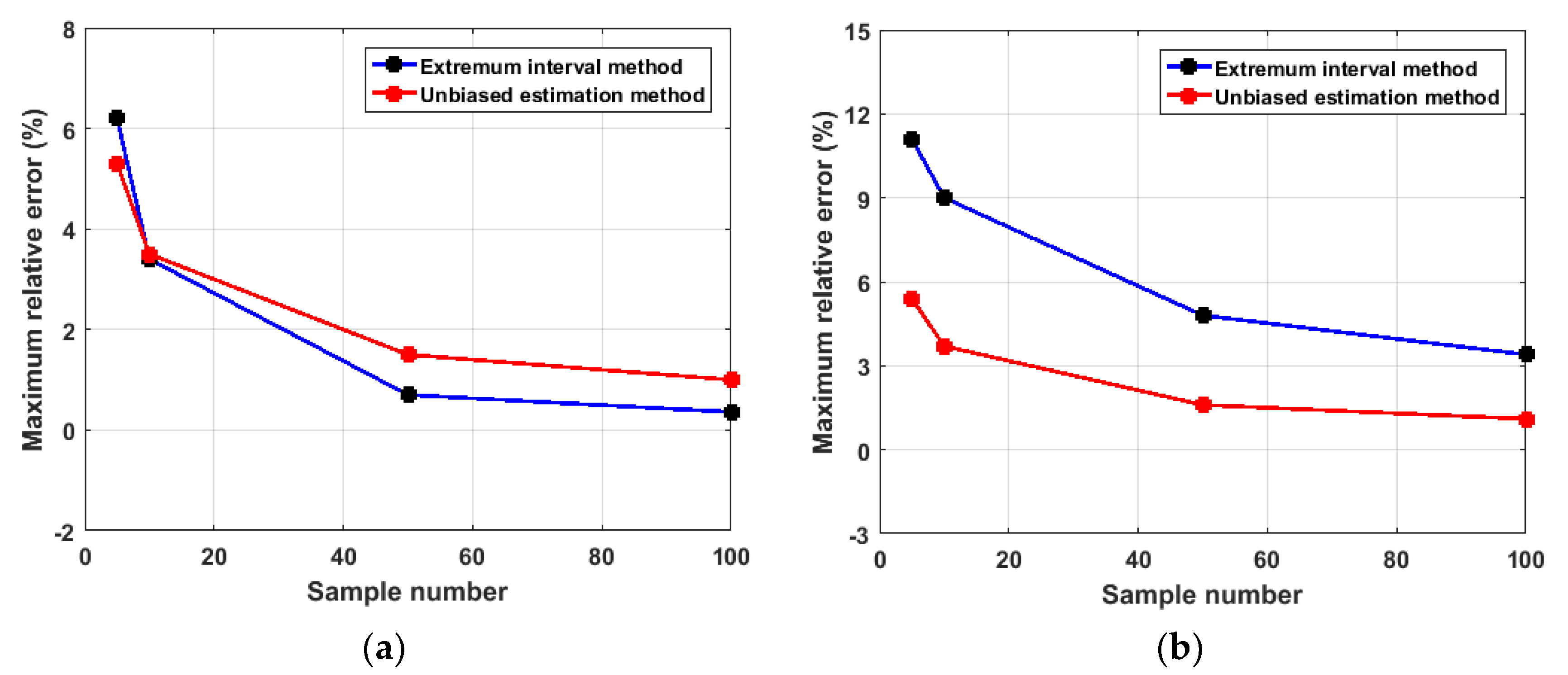
3.3. Unbiased Estimation for Inadequate Interval

For practical engineering systems, the traditional extremum interval method maybe not cover the factual data accurately. Hence, for the condition with limited data, the unbiased estimation method will be adopted to handle this small sample problem. According to the distribution of available experimental data, it can be roughly divided into two forms: uniform distribution and normal distribution.

3.3.1. Uniformly Distributed

If the experiment data have been provided as a sample set $\left\{t_1,t_2,\cdot \cdot \cdot ,t_n\right\}$, and all samples are uniformly distributed within the interval $[\underset{\_}{T},\overline{T}]$, then, the theoretical mean and variance of $T$ can be expressed as

$$E(T)=\frac{\underset{\_}{T}+\overline{T}}{2}\hspace{1em}Var(T)=\frac{{(\overline{T}-\underset{\_}{T})}^2}{12}$$

(22)

Then, the unbiased estimation bounds of the limited experiment observations can be calculated

$${\underset{\_}{T}}^u=\frac{1}{n}{\displaystyle \sum _{i=1}^n{t}_i}-\sqrt{\frac{3}{n-1}\cdot {\displaystyle \sum _{i=1}^n{(t_i-{\overline{T}}^M)}^2}}\hspace{1em}{\overline{T}}^u=\frac{1}{n}{\displaystyle \sum _{i=1}^n{t}_i}+\sqrt{\frac{3}{n-1}\cdot {\displaystyle \sum _{i=1}^n{(t_i-{\overline{T}}^M)}^2}}$$

(23)

where superscript u and M denote unbiased estimation and experiment measurements, respectively, its derivation is given in Appendix A.

3.3.2. Normal Distribution

Similarly, if the experiment data have been provided as a sample set $\left\{t_1,t_2,\cdot \cdot \cdot ,t_n\right\}$, and each sample is normal distributed in the interval $[\underset{\_}{T},\overline{T}]$. The unbiased estimation of mean and variance of $T$ can be derived as follows.

$$E(T)={\overline{T}}^M\approx \frac{1}{n}{\displaystyle \sum _{i=1}^n{t}_i}\hspace{1em}Var(T)\approx \frac{1}{n-1}{\displaystyle \sum _{i=1}^n{(t_i-{\overline{T}}^M)}^2}$$

(24)

According to the distribution characteristics of normal distributed, the unbiased estimation bounds of the limited experiment observations can be calculated

$${\underset{\_}{T}}^u=\frac{1}{n}{\displaystyle \sum _{i=1}^n{t}_i}-3\cdot \sqrt{\frac{1}{n-1}\cdot {\displaystyle \sum _{i=1}^n{(t_i-{\overline{T}}^M)}^2}}\hspace{1em}{\overline{T}}^u=\frac{1}{n}{\displaystyle \sum _{i=1}^n{t}_i}+3\cdot \sqrt{\frac{1}{n-1}\cdot {\displaystyle \sum _{i=1}^n{(t_i-{\overline{T}}^M)}^2}}$$

(25)

From the operation mentioned above, the interval bounds of experimental observations can be estimated, which will be more practical for the engineering system with limited experimental measurements compared to the traditional extremum interval method.

3.3.3. Numerical Calculation

For the basic distribution laws described above, the numerical example was provided to verify the effectiveness of the proposed unbiased estimation method.

Assume the sample changes within the interval [50, 60], where we repeat 100 times to calculate the average maximum relative error.

Note from Figure 5, both unbiased estimation methods can better describe the actual measurement interval in the case of small samples. With increase of sample number, the uniformly distributed-based unbiased estimation can not show better performance compared with the extremum interval method. However, the normal distributed-based unbiased estimation can always maintain an excellent estimation performance.

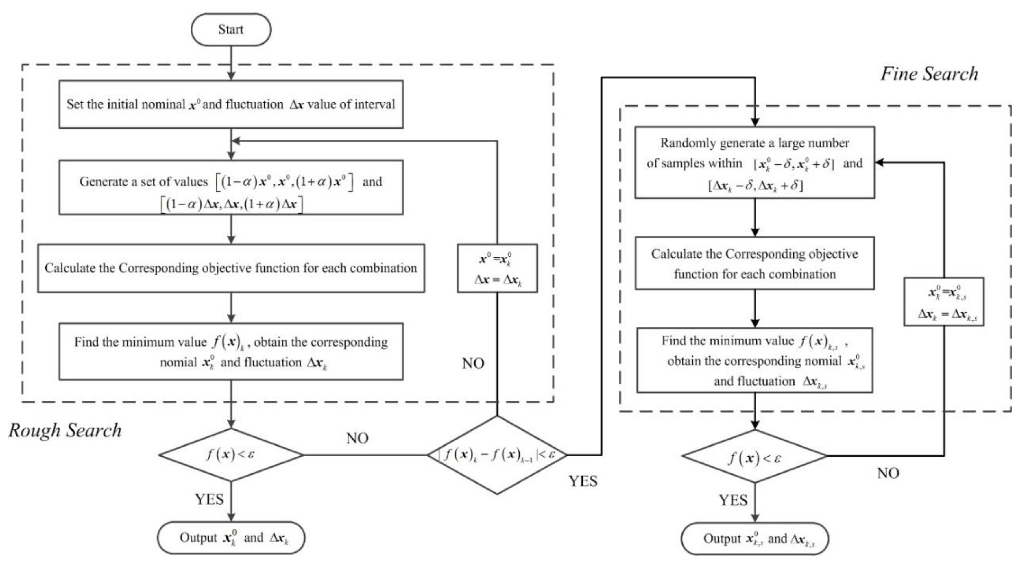
4. Interval Parameter Identification Procedure

This section introduces a novel interval parameter identification method, which adopted the improved optimization strategy. Similar to the traditional parameter identification, the system with uncertainty can be implemented effectively by converting into an inverse optimization problem, which seeks the minimum relative error between the calculated value and experimental value. The mathematical model of the optimization process can be expressed in the following general form:

$$\begin{array}{l}Find\mathit{x}={\left\{\left[\underset{\_}{x_i},\overline{x_i}\right]\right\}}_m\\ \min f\left(\mathit{x}\right)={\displaystyle \sum _{i=1}^n\left(\left|\left(T_i{}^P\left(\mathit{x}\right)-T_i{}^M\right)/T_i{}^M\right|\right)}\\ ={\displaystyle \sum _{i=1}^n\left(\left|\left({\underset{\_}{T_i}}^P(\mathit{x})-{\underset{\_}{T_i}}^M\right)/{\underset{\_}{T_i}}^M\right|+\left|\left({\overline{T_i}}^P(\mathit{x})-{\overline{T_i}}^M\right)/{\overline{T_i}}^M\right|\right)}\\ s.t.\underset{\_}{\mathit{x}}\le \mathit{x}\le \overline{\mathit{x}}\end{array}$$

(26)

where $\mathit{x}$ denotes the system unknown parameter vector, $m$ and $n$ is the number of unknown parameters and system features, respectively, $f\left(\mathit{x}\right)$ describes the relative error of system, and the superscript P and M stands for the predicted and measured value, respectively.

As seen in Figure 6, the process of the interval parameter identification is clearly shown. Among them, several judgment conditions are set to ensure the effective operation of the procedure. Specifically, the “Condition met” in the step of construct the surrogate model guarantees the accuracy of the ATP model. While, the judgment follows the step of updating strategy is set to ensure that the ATP model can maintain high accuracy throughout the optimization process. The proposed interval parameter identification method roughly consists of two parts: (1), searching the initial value of the variable; (2), performing the rough and fine search to obtain the identified result.

4.1. Searching the Initial Value

In this step, the interval parameter identification process was executed by converting into a deterministic framework problem, which was used to seek the initial value of unknown parameters corresponding to the mean of measurement intervals. Hence, the optimization model can be expressed as follows:

$$\begin{array}{l}Find\mathit{x}={\left\{x_i\right\}}_m\\ \min f\left(\mathit{x}\right)={\displaystyle \sum _{i=1}^n\left(\left|\left(T_i{}^P\left(\mathit{x}\right)-T_i{}^{Mmean}\right)/T_i{}^{Mmean}\right|\right)}\\ s.t.\underset{\_}{\mathit{x}}\le \mathit{x}\le \overline{\mathit{x}}\end{array}$$

(27)

where $T_{}{}^{Mmean}$ describes the mean of measurements interval, $T_{}{}^P\left(\mathit{x}\right)$ denotes the predicted value of system.

The traditional optimization algorithms can be applied to this process, such as exhaustive method, particle swarm algorithm, and genetic algorithm. By executing this step, the initial value of unknown parameters can be obtained, which can provide an initial identification range for subsequent calculations.

4.2. Searching the Eventual Result

In contrast to the deterministic framework, the traditional optimization algorithms may not be able to deal with the uncertain system better. To improve the accuracy and efficiency of the parameter identification, the multi-level optimization-based strategy was constructed, which mainly included two steps: rough search and fine search.

Note from Figure 7, the procedure is executed in the order of rough search and fine search. In the rough search, the initial interval of unknown parameters is defined according to the value calculated above. By introducing the constriction factor, the process of rough search can obtain a group of identification results rapidly. If the result can not meet the requirement of precision, the procedure will automatically move to the stage of the fine search. In this stage, numerous samples will be randomly generated near the above identification results to search the optimal results. The detailed process is shown in Figure 7.

For the calculation of the system predicted interval, various methods have been tried, for instance, interval arithmetic, series expansion, perturbation, optimization, among others. However, these methods cannot show active inclusiveness for solving complex nonlinear problems. Therefore, Monte Carlo is adopted as a simple and effective method. By sampling a large number of parameter intervals, the interval of the objective function can be calculated rapidly. The proposed multi-level optimization-based strategy can identify the unknown parameter of uncertain systems efficiently and accurately.

5. Numerical Example

A box structure made of metal-foam was provided to verify the efficiency of the proposed method. In order to improve computational efficiency, the equivalent solid parameter model was adopted, where the actual performance of metal-foam structure can be simulated by adjusting the thermodynamic parameters of the equivalent model. The schematic diagram of the structure was shown in Figure 8, where the overall dimensions were 500 mm × 500 mm × 500 mm, and the thickness was 30 mm. Meanwhile, there is a 100 × 100 × 100 mm heating element on the middle of the bottom. The whole structure is made of the same material with emissivity $\epsilon$ and heat conductivity k. To simulate the heat transfer performance of the box under low temperature and pressure environment at high altitudes, the ambient air temperature outside the box is set to –60 °C, and the initial ambient air temperature in the box is set to 20 °C. Besides, the combination of radiation and convection was considered both inside and outside the box, where the external convection heat transfer coefficient was set to $3\mathrm{W}/({\mathrm{m}}^2\cdot \mathrm{K})$. Then, the finite element model of equivalent model was created in NX THERMAL/FLOW with 14,049 tetrahedron elements and 27,302 nodes, as shown in Figure 8b. Four nodes were selected as the feature response points, where point 1 and 2 were located at the center of the outer surface of the box, respectively, and point 3 and 4 were distributed along the centerline at the inner surface of the box, as shown in Figure 8a. And the temperature value of each feature point is the result of the steady state of the system. Furthermore, it should be noted that the thermodynamic parameters identified by this method are not parameters of metal-foam models, but the equivalent model. In other words, we can obtain a more accurate equivalent model that can simulate the original foam structure.

Due to the uncertainty of the metal-foam material properties, as well as the uncertainty of the complicated external factors, various uncertainties unavoidably exist in the heat transfer system of the box structure. According to the description in Section 2, if the equivalent heat conductivity, emissivity and the power of heating element are known in advance to change in the intervals $k\in [10,20]\mathrm{W}/(\mathrm{m}\cdot \mathrm{K})$, $\epsilon \in [0.4,0.8]$, and $\mathrm{p}\in [10,15]\mathrm{W}$, the accurate intervals of four feature points can be calculated by the optimization algorithm, where the temperature responses are changed in the ranges [−56.85, −49.57], [−49.80, −34.97], [−56.56, −49.11], [−55.36, −47.83] respectively.

In order to simulate the situation lack of measurement datas in actual engineering, 8 samples of each temperature response intervals are randomly selected with the assumption of normal distribution, which are listed in Equation (28).

$$\begin{array}{l}{T}_1=\left\{-53.85,-54.21,-53.33,-55.12,-53.21,-54.86,-51.04,-54.10\right\};\\ T_2=\left\{-44.20,-42.96,-41.46,-38.40,-41.33,-45.14,-39.02,-43.78\right\};\\ T_3=\left\{-52.01,-54.25,-54.68,-54.90,-52.94,-53.53,-51.10,-53.04\right\};\\ T_4=\left\{-52.39,-50.32,-50.97,-50.62,-53.11,-51.30,-51.70,-53.31\right\};\end{array}$$

(28)

By utilizing the traditional extremum description method, the intervals of above sample set can be described as

$$\begin{gathered} T_1^e=[-55.12,-51.04]\hspace{1em}{T}_2^e=[-45.14,-38.40] \\ {T}_3^e=[-54.90,-51.10]\hspace{1em}{T}_4^e=[-53.31,-50.32] \end{gathered}$$

(29)

Similarly, the unbiased estimation method is applied to obtain the unbiased intervals of the above sample set, which shown in Equation (30).

$$\begin{gathered} T_1^u=[-57.51,-49.91]\hspace{1em}{T}_2^u=[-49.33,-34.74] \\ {T}_3^u=[-57.25,-49.36]\hspace{1em}{T}_4^u=[-55.08,-48.34] \end{gathered}$$

(30)

In contrast to the temperature response intervals calculated by the traditional extremum description method, the unbiased intervals are closer to the original intervals, which illustrate the efficiency of the unbiased estimation method for the actual engineering with inadequate information.

After performing the process of parameter identification, the eventually identified results of heat conductivity, emissivity, and the power of the heating element are listed in

Table 1. Identified results of the box heat transfer system.

Parameter	Real Interval	Identification Interval	Error (%)
k(W/(m·°C))	[10, 20]	[9.62, 19.56]	(3.8, 2.2)
ε	[0.4, 0.8]	[0.4159, 0.8241]	(3.9, 3.0)
P (W)	[10, 15]	[10.57, 15.21]	(5.7, 1.4)
Mean			(4.5, 2.2)

. Meanwhile, the corresponding response intervals of the four feature points can be seen in

Table 2. Temperature intervals of the box heat transfer system.

Feature	Real Interval	Unbiased Interval	Output Interval	Error (%)
Point 1	[−56.85, −49.57]	[−57.51, −49.91]	[−56.75, −49.83]	(0.1759, −0.5245)
Point 2	[−49.80, −34.97]	[−49.33, −34.74]	[−49.34, −34.72]	(0.9237, 0.7149)
Point 3	[−56.56, −49.11]	[−57.25, −49.36]	[−56.47, −49.36]	(0.1591, −0.5091)
Point 4	[−55.36, −47.83]	[−55.08, −47.35]	[−55.23, −47.83]	(0.2348, 0)
Mean				(0.3734, 0.4371)

. The mean relative errors of the parameter intervals and the temperature response intervals are dramatically reduced to (4.5, 2.2)% and (0.3734, 0.4371)%, respectively. Note from Figure 9 that the system response intervals can converge rapidly in the identification process where the error can be reduced quickly in the stage of the rough search, while in the fine search stage, the error tends to converge gradually, which demonstrates the efficiency of the proposed optimization strategy. Moreover, Figure 10, Figure 11 and Figure 12 show the initial, true, and identification space of the temperature response, where the identified results can better match the real results. Therefore, the proposed interval parameter identification method can be effectively applied to the actual heat transfer problem with uncertainty.

6. Conclusions

Firstly, this work presents a novel modelling methodology for low porosity metal-foam materials, and for the heat transfer system of metal-foam structure, develops a novel interval parameter identification method, which can quantify the uncertainty parameters in the actual engineering problems with only limited experimental measurements effectively. In summary, the conclusions can be drawn:

• A novel Voronoi-based modelling methodology is proposed for the closed-cell metal-foam in low porosity, by which the realistic pore geometry can be generated concisely and effectively. This method adopts the new algorithm of spheres random packing, which can simplify the calculation program. Moreover, the randomness of the boundary thickness between pores is taken into account in the searching process. Meanwhile, the boundary constraint can be effectively removed when searching the maximum volume sphere of convex polyhedra on boundary surfaces.
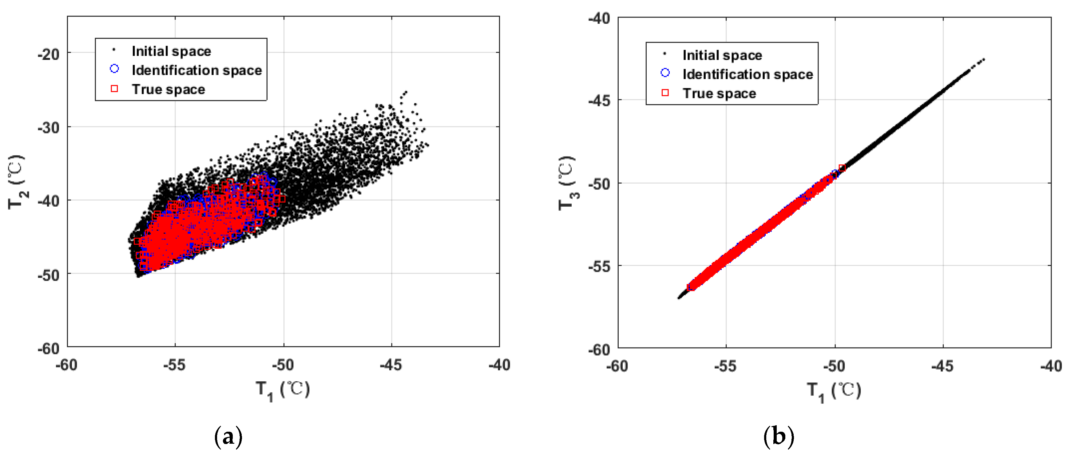
• Compared to the probabilistic based parameter identification methods, interval methods can preferably describe uncertainty problems, especially for the case with limited information. Besides, the novel ATP surrogate model was constructed to describe the mapping relationship between variables and responses effectively and accurately. Meanwhile, the unbiased estimations method is adopted to describe the measurement interval of the actual engineering system accurately.
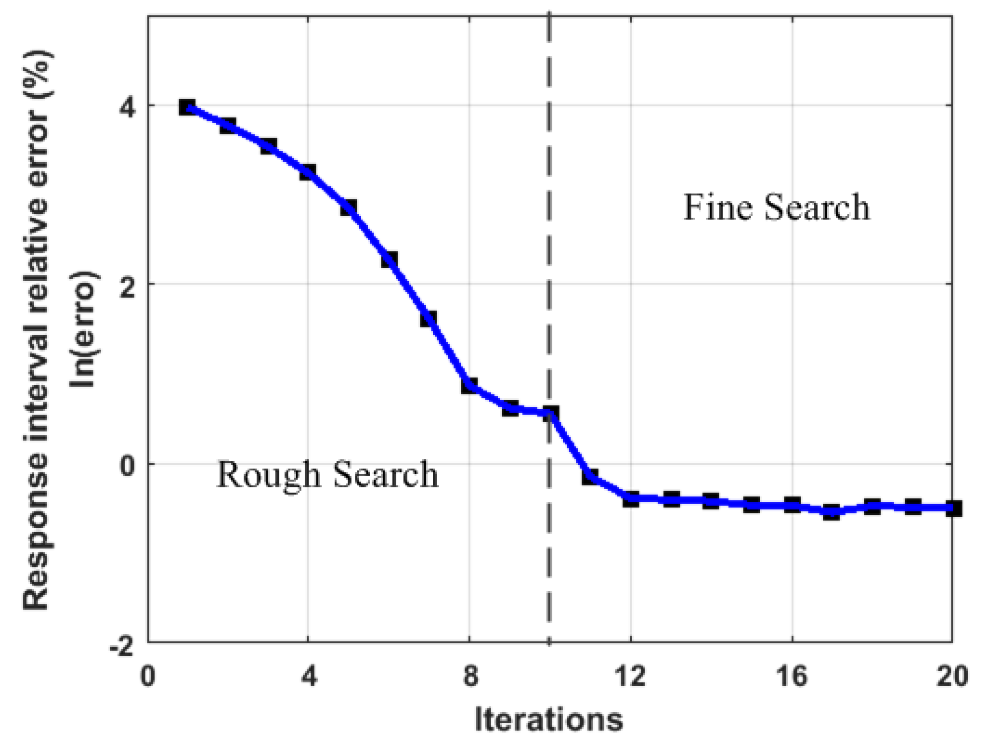
• To executive the parameter identification procedure effectively, the novel multi-level optimization-based strategy was designed, which can identify the unknown parameter of uncertain systems efficiently and accurately in the order of searching the initial value, rough searching, and fine searching.
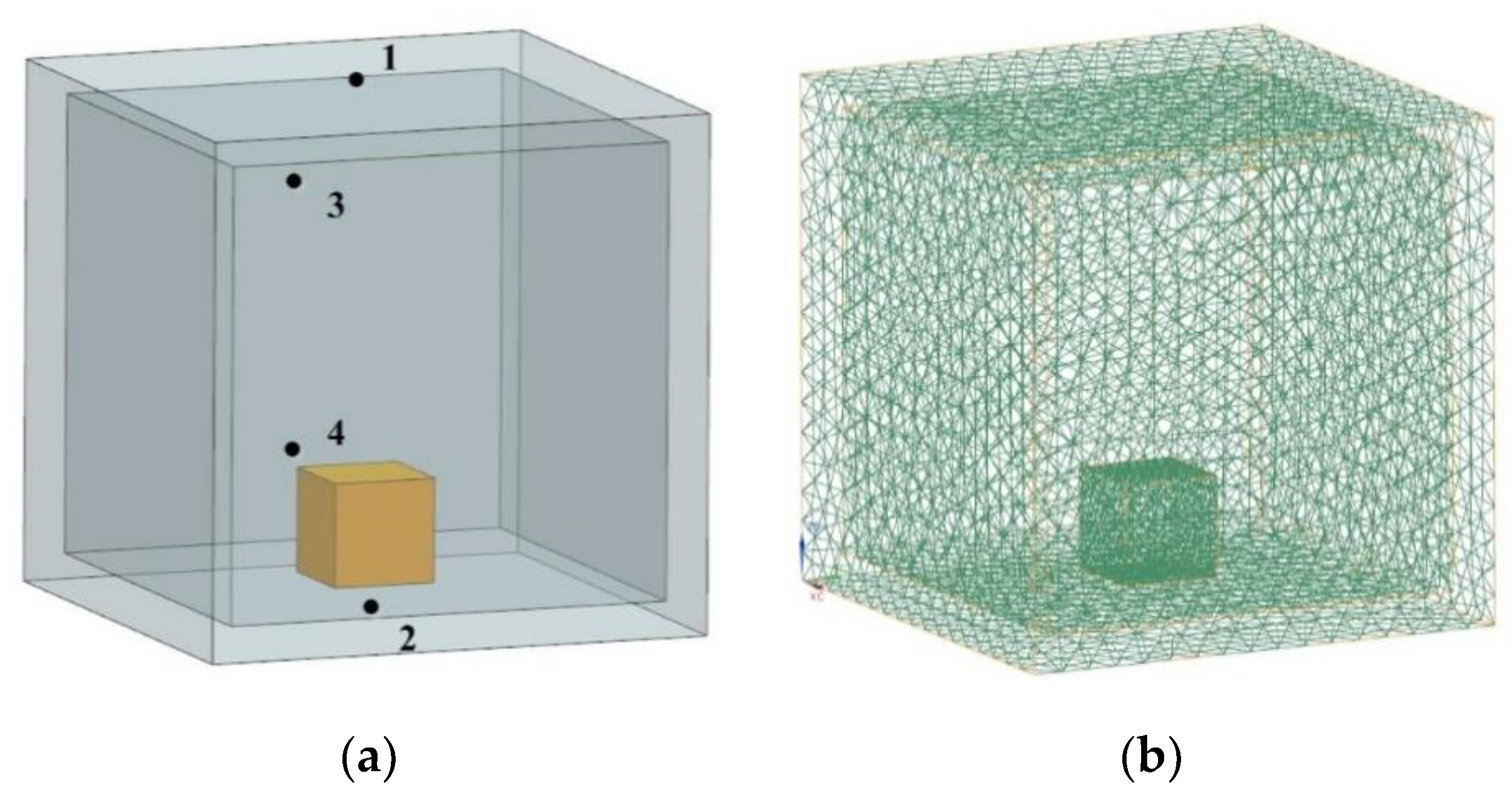
• An engineering heat transfer example of a box structure made of metal-foam was provided to verify the efficiency of the proposed method without sufficient information. The satisfactory identification results were obtained when applied to the proposed method, which indicated that the proposed interval parameter identification method could quantify the uncertainty of metal-foam structure in the engineering heat transfer system efficiently, especially for the actual case without sufficient measurements.
• The application of the unbiased estimation method was under certain conditions in this study. Furthermore, the validation example just considered a single non-probabilistic uncertainty. In the future, the applicable conditions of the unbiased estimation method will be further studied. Meanwhile, the proposed method will be expanded to complex engineering problems with mixed uncertainties.

References

1. Gibson, L.J.; Ashby, M.F. Cellular Solids Structure and Properties, 2nd ed.; Cambridge University Press: Cambridge, UK, 1997. [Google Scholar]
2. Silva, M.J.; Gibson, L.J. The effects of non-periodic microstructure and defects on the compressive strength of two-dimensional cellular solids. Int. J. Mech. Sci. 1997, 39, 549–563. [Google Scholar] [CrossRef]
3. Wang, J.G.; Sun, W.; Anand, S. Amicrostructure analysis for crushable deformation of foammaterials. Comput. Mater. Sci. 2008, 44, 195–200. [Google Scholar] [CrossRef]
4. Gibson, L.J.; Ashby, M.F. The mechanics of three-dimensional cellularmaterials. Proc. R. Soc. 1982, 382, 43–59. [Google Scholar]
5. Demiray, S.; Becker, W.; Hohe, J. Numerical determination of initial and subsequent yield surfaces of open-celled model foams. Int. J. Solids Struct. 2007, 44, 1093–1208. [Google Scholar] [CrossRef]
6. Liu, P.S. Failure by buckling mode of the pore-strut for isotropic three-dimensional reticulated porous metal foams under different compressive loads. Mater. Des. 2011, 32, 3493–3498. [Google Scholar] [CrossRef]
7. Sassov, A.; Cornelis, E.; Dyck, D. Non-destructive 3D investigation of metal foam microstructure. Mater. Werkst. 2000, 31, 571–573. [Google Scholar] [CrossRef]
8. Toda, H.; Ohgaki, T.; Uesugi, K.; Makii, K.; Aruga, Y.; Akahori, T.; Niinomi, M.; Kobayashi, T. In situ observation of fracture of aluminium foam using synchrotron X-ray microtomography. Key Eng. Mater. 2005, 297, 1189–1195. [Google Scholar] [CrossRef]
9. Miedzinska, D.; Niezgoda, T.; Gieleta, R. Numerical and experimental aluminum foam microstructure testing with the use of computed tomography. Comput. Mater. Sci. 2012, 64, 90–95. [Google Scholar] [CrossRef]
10. Ramirez, J.F.; Cardona, M.; Velez, J.A.; Mariaka, I.; Isaza, J.A.; Mendoza, E.; Betancourt, S.; Fernández-Morales, P. Numerical modeling and simulation of uniaxial compression of aluminum foams using FEM and 3D-CT images. Proc. Mater. Sci. 2014, 4, 227–231. [Google Scholar] [CrossRef] [Green Version]
11. Islam, M.A.; Brown, A.D.; Hazell, P.J.; Kader, M.A.; Escobedo, J.P.; Saadatfar, M.; Xu, S.; Ruan, D.; Turner, M. Mechanical response and dynamic deformation mechanisms of closed-cell aluminium alloy foams under dynamic loading. Int. J. Impact Eng. 2018, 114, 111–122. [Google Scholar] [CrossRef]
12. Sharma, V.; Zivic, F.; Grujovic, N.; Babcsan, N.; Babcsan, J. Numerical Modeling and Experimental Behavior of Closed-Cell Aluminum Foam Fabricated by the Gas Blowing Method under Compressive Loading. Materials 2019, 12, 1582. [Google Scholar] [CrossRef] [PubMed] [Green Version]
13. Wejrzanowski, T.; Skibinski, J.; Szumbarski, J.; Kurzydlowski, K.J. Structure of foams modeled by Laguerre-Voronoi tessellations. Comput. Mater. Sci. 2013, 67, 216–221. [Google Scholar] [CrossRef]
14. Tang, L.; Shi, X.; Zhang, L.; Liu, Z.; Jiang, Z.; Liu, Y. Effects of statistics of cell’s size and shape irregularity on mechanical properties of 2D and 3D Voronoi foams. Acta Mech. 2014, 225, 1361–1372. [Google Scholar] [CrossRef]
15. Yang, B.; Liu, Z.J.; Tang, L.Q.; Jiang, Z.Y.; Liu, Y.P. Mechanism of the strain rate effect of metal foams with numerical simulations of 3D Voronoi foams during the split Hopkinson pressure bar tests. Int. J. Comput. Methods 2015, 12. [Google Scholar] [CrossRef]
16. Zhang, X.T.; Wang, R.Q.; Liu, J.X.; Li, X.; Jia, G. A numerical method for the ballistic performance prediction of the sandwiched open cell aluminum foam under hypervelocity impact. Aerosp. Sci. Technol. 2018, 75, 254–260. [Google Scholar] [CrossRef]
17. Zhang, Y.; Jin, T.; Li, S.Q.; Ruan, D.; Wang, Z.; Lu, G. Sample size effect on the mechanical behavior of aluminum foam. Int. J. Mech. Sci. 2019, 151, 622–638. [Google Scholar] [CrossRef]
18. Skibinski, J.; Cwieka, K.; Ibrahim, S.H.; Wejrzanowski, T. Influence of Pore Size Variation on Thermal Conductivity of Open-Porous Foams. Materials 2019, 12, 12. [Google Scholar] [CrossRef] [Green Version]
19. Alexander, Z.; Zinchenko. Algorithm for Random Close Packing of Spheres with Periodic Boundary Conditions. J. Comput. Phys. 1994, 114, 298–307. [Google Scholar]
20. Fang, Q.; Zhang, J.H.; Chen, L.; Liu, J.; Fan, J.; Zhang, Y. An algorithm for the grain-level modelling of a dry sand particulate system. Model. Simul. Mater. Sci. Eng. 2014, 22, 5. [Google Scholar] [CrossRef]
21. Zheng, Z.J.; Wang, C.F.; Yu, J.L.; Rei, S.R.; Harriga, J.J. Dynamic stress–strain states for metal foams using a 3D cellular model. J. Mech. Phys. Solids 2014, 72, 93–114. [Google Scholar] [CrossRef]
22. Khodaparast, H.H.; Mottershead, J.E.; Friswell, M.I. Perturbation methods for the estimation of parameter variability in stochastic model updating. Mech. Syst. Signal Process. 2008, 22, 1751–1773. [Google Scholar] [CrossRef]
23. Deng, Z.M.; Bi, S.F.; Atamturktur, S. Stochastic model updating using distance discrimination analysis. Chin. J. Aeronaut. 2014, 27, 1188–1198. [Google Scholar] [CrossRef] [Green Version]
24. Zhang, W.; Liu, J.; Cho, C.; Han, X. A hybrid parameter identification method based on Bayesian approach and interval analysis for uncertain structures. Mech. Syst. Signal Process. 2015, 60, 853–865. [Google Scholar] [CrossRef]
25. Wu, Z.F.; Huang, B.; Li, Y.J.; Pu, W. A Statistical Model Updating Method of Beam Structures with Random Parameters under Static Load. Appl. Sci. 2017, 7, 6. [Google Scholar] [CrossRef] [Green Version]
26. Furukawa, T.; Lim, S.H.; Michopoulos, J.G. Stochastic identification of defects under sensor uncertainties. Int. J. Numer. Methods Eng. 2012, 90, 135–151. [Google Scholar] [CrossRef]
27. Wan, H.P.; Ren, W.X. Stochastic model updating utilizing Bayesian approach and Gaussian process model. Mech. Syst. Signal Process. 2016, 70–71, 245–268. [Google Scholar] [CrossRef]
28. Wang, C.; Matthies, H.G.; Qiu, Z.P. Optimization-based inverse analysis for membership function identification in fuzzy steady-state heat transfer problem. Struct. Multidiscip. Optim. 2018, 57, 1495–1505. [Google Scholar] [CrossRef]
29. Fedele, F.; Muhanna, R.L.; Xiao, N.; Mullen, R.L. Interval-based approach for uncertainty propagation in inverse problems. J. Eng. Mech. 2014, 141, 1–7. [Google Scholar] [CrossRef]
30. Chen, X.; Shen, Z.; Liu, X. A Copula-Based and Monte Carlo Sampling Approach for Structural Dynamics Model Updating with Interval Uncertainty. Shock and Vibration. 2018, 2018. [Google Scholar] [CrossRef] [Green Version]
31. Liu, Y.S.; Wang, X.J.; Wang, L. Interval uncertainty analysis for static response of structures using radial basis functions. Appl. Math. Model. 2019, 69, 425–440. [Google Scholar] [CrossRef]
32. Zheng, Z.L.; Jing, Q.; Xie, Y.H.; Zhang, D. An Investigation on the Forced Convection of Al2O3-water Nanofluid Laminar Flow in a Microchannel under Interval Uncertainties. Appl. Sci. 2019, 9, 3. [Google Scholar] [CrossRef] [Green Version]
33. Khodaparast, H.H.; Mottershead, J.E.; Badcock, K.J. Interval model updating with irreducible uncertainty using the Kriging predictor. Mech. Syst. Signal Process. 2011, 25, 1204–1226. [Google Scholar] [CrossRef]
34. Fang, S.E.; Zhang, Q.H.; Lin, Y.Q.; Ren, W.X. An interval model updating strategy using interval response surface models. Mech. Syst. Signal Process. 2015, 60–61, 909–927. [Google Scholar] [CrossRef]
35. Deng, Z.M.; Guo, Z.P. Interval identification of structural parameters using interval overlap ratio and Monte Carlo simulation. Adv. Eng. Softw. 2018, 21, 120–130. [Google Scholar] [CrossRef]
36. Deng, Z.M.; Guo, Z.P.; Zhang, X.J. Interval model updating using perturbation method and radius basis function neural networks. Mech. Syst. Signal Process. 2017, 84, 699–716. [Google Scholar] [CrossRef]
37. Chong, W.; Hermann, G.M. Novel interval theory-based parameter identification method for engineering heart transfer systems with epistemic uncertainty. Int. J. Numer. Methods Eng. 2018, 115, 756–770. [Google Scholar]
38. Wang, X.G.; He, W.L.; Zhao, L.G. Novel Interval Parameter Identification Method Using Augmented Fourier Series-Based Polynomial Surrogate Model. IEEE Access 2019, 7, 70862–70875. [Google Scholar]
39. Zhao, A.; Hu, Y.B. Numerical Simulation of Effective Thermal Conductivity Aluminum Foam Sandwich Panel. Thermodynamics 2018, 22, 2827–2834. [Google Scholar] [CrossRef]
40. Solorzano, E.; Reglero, J.A.; Rodriguez-Perez, M.A.; Lehmhus, D.; Wichmann, M.; de Saja, J.A. An experimental study on the thermal conductivity of foams by using the transient plane source method. Int. J. Heat Mass Transf. 2008, 51, 6259–6267. [Google Scholar] [CrossRef]
41. Wang, H.; Liu, B.; Kang, Y.X.; Qin, Q.H. Analysing effective thermal conductivity of 2D closed-cell foam based on shrunk Voronoi tessellations. Arch. Mech. 2017, 69, 451–470. [Google Scholar]
42. Liu, Z.Z.; Wang, T.S.; Li, J.F. A trigonometric interval method of dynamic response analysis of uncertain nonlinear systems. Sci. China Phys. Mech. Astron. 2015, 58, 044501. [Google Scholar] [CrossRef]
Figure 1. Operation in MATLAB: (a) Voronoi tessellation; (b) Spheres random packing.
Applsci 10 01429 g001
Figure 2. Operation in UG: (a) 3D pore solid model; (b) Metal-foam solid model.
Applsci 10 01429 g002
Figure 3. Models’ predictions and measurement and simulation value of thermal conductivity of metal-foam with different porosity.
Applsci 10 01429 g003
Figure 4. Approximation of f ( x ) : (a) 5 order approximation of various basis functions; (b) Approximation error of various basis functions.
Applsci 10 01429 g004
Figure 5. Maximum relative error of unbiased estimation method: (a) Uniformly distributed; (b) Normal distribution.
Applsci 10 01429 g005
Figure 6. Flowchart of the system interval parameter identification.
Applsci 10 01429 g006
Figure 7. Flowchart of the parameter interval updating strategy.
Applsci 10 01429 g007
Figure 8. The box structures: (a) Entity model; (b) Finite element model.
Applsci 10 01429 g008
Figure 9. Convergence processes of temperature response relative error in the heat transfer system.
Applsci 10 01429 g009
Figure 10. The initial, true, and identification space in the heat transfer system: (a) Temperature response T1–T2; (b) Temperature response T1–T3.
Applsci 10 01429 g010
Figure 11. The initial, true, and identification space in the heat transfer system: (a) Temperature response T1–T4; (b) Temperature response T2–T3.
Applsci 10 01429 g011
Figure 12. The initial, true, and identification space in the heat transfer system: (a) Temperature response T2–T4; (b) Temperature response T3–T4.
Applsci 10 01429 g012