Abstract
Due to the high cost of failures of wind turbines, redundancy designs are commonly applied in wind turbines for improving the reliability and availability of systems. For this reason, replacing failed components with other working components of the same type in redundant systems is becoming an attractive option of maintenance strategies towards more resilient systems. To quantitatively evaluate system’s reliability, this paper focuses on the reliability analysis of redundant systems of offshore wind turbines based on swapping existing components. The survival signature-based component swapping method is introduced to describe the new structure-function of the system upon swapping. Furthermore, the reliability model of redundant systems is established using the fault tree and survival signature. Following this, the influences of component swapping on component reliability importance measure (marginal reliability importance and joint reliability importance) without and with considerations of the imprecision of failure rates are explored. Finally, a 5MW offshore wind turbine is presented to show the applicability of the proposed approach for redundant systems, and the results show that the proposed approach can obtain realistic reliability assessment of redundant systems and considering component swapping can significantly improve system reliability.
1. Introduction
As climate change and energy crises continue to worsen worldwide, there is an increased eagerness to develop cleaner alternatives to fossil fuels. Wind energy is one of the most promising renewable energy sources. Nowadays, the power and complexity of wind turbines (WTs) are rapidly increasing. Complex electromechanical systems and uncertainties of extreme operating environments of wind turbines lead to serious accidents resulting in huge economic losses and threats to human lives [1,2,3].
To eliminate the weaknesses in complex system, redundancy designs are widely used for the improvement of system reliability and availability. In engineering practice, active redundancy, passive redundancy, partly loaded redundancy, and change over redundancy are commonly applied to enhance system reliability [4,5,6]. Reliability-redundancy allocation aims to obtain the optimal redundancy level of each subsystem to maximize the system reliability within allowable resources of the entire system [7,8]. However, most redundant components have been treated as a parallel configuration without considerations of the failure mechanism of redundant systems [5]. Survival signature-based reliability analysis method has been applied to systems with multiple types of components, and excellent results are also achieved [9,10,11].
Many researchers have previously studied reliability importance analysis (Marginal reliability importance (MRI) and Joint reliability importance (JRI)) and reliability sensitivity analysis for complex systems. Hong & Lie [12], and Armstrong [13] introduced the JRI to explore how two components in a system interact in contributing to the system’s reliability. The JRI was extended from two components to multi-components [14]. Feng et al. [15] used the survival signature to perform imprecise system reliability analysis and component importance analysis. Xu and Liao [16] studied the reliability of a one-shot system containing multi-functional components. Huang et al. [17,18] performed the reliability sensitivity analysis for coherent systems using survival signature and system reliability optimization considering swapping existing components. However, the effects of component swapping on system reliability and component importance have not been extensively studied in the existing literature.
In reality, components swapping is of great importance in improving the reliability of redundant systems, i.e., offshore wind turbines, which have high-reliability requirements. Due to the scale and complexity of the redundancies in complex systems, it is a challenge for us to express the change of the structure function of redundant systems upon swapping, which causes the fact that the system reliability with component swapping can not be realistically evaluated. Furthermore, the quantitative measure of MRI and JRI of redundant components can help allocate resources (design, inspection and maintenance) reasonably. However, the listed literature did not explore the influences of component swapping on system reliability, MRI and JRI of critical components. Moreover, the uncertainties of failure rates of components were not studied.
Component swapping developed from survival signature is an effective method to enhance system reliability by swapping between failed components and working components of the same types in a redundant system, which can significantly improve the resilience of systems to failures [19]. Actually, this kind of maintenance strategy is already used to prevent the shutdown of wind turbines and avoid huge losses in reality. However, the influences of components swapping on system reliability have not yet been explored due to the change of system structure upon swapping. Moreover, the MRI and JRI with considerations of component swapping and fuzzy failure rates can not be conducted as well. To realistically and quantitatively evaluate the reliability of redundant systems, in this paper, authors therefore propose to establish a time-dependent reliability model for redundant systems of a 5 MW offshore wind turbine based on component swapping. Reliability functions of load-sharing and standby redundant systems are derived. Effects of component swapping on the reliability of redundant systems are explored. Component reliability importance measure considering component swapping and imprecise failure rates is performed. The MRI and JRI of critical components considering component swapping are analyzed, and the lower and upper bounds of MRI and JRI of critical components are presented using imprecise theory.
The rest of this paper is organized as follows: Section 2 introduces redundant systems and the fault tree of offshore wind turbines; Section 3 describes methods mentioned in this study including component swapping, reliability importance analysis, reliability functions of load-sharing redundancy and standby redundancy; Section 4 presents system reliability model and results analysis; Section 5 performs reliability importance analysis of redundant components of different types; Finally, some conclusions are summarized in Section 6.
2. Redundant Systems of Offshore Wind Turbines
An offshore wind turbine is taken as an example to show the effectiveness and feasibility of the proposed methods. In the wind-power industry, redundancy designs play an important role in improving the system reliability of wind turbines. The redundancy of a component or system can improve the ability to maintain or restore its function when a failure of a member or connection has occurred. Redundancy can be achieved for instance by strengthening or introducing alternative load paths [20].
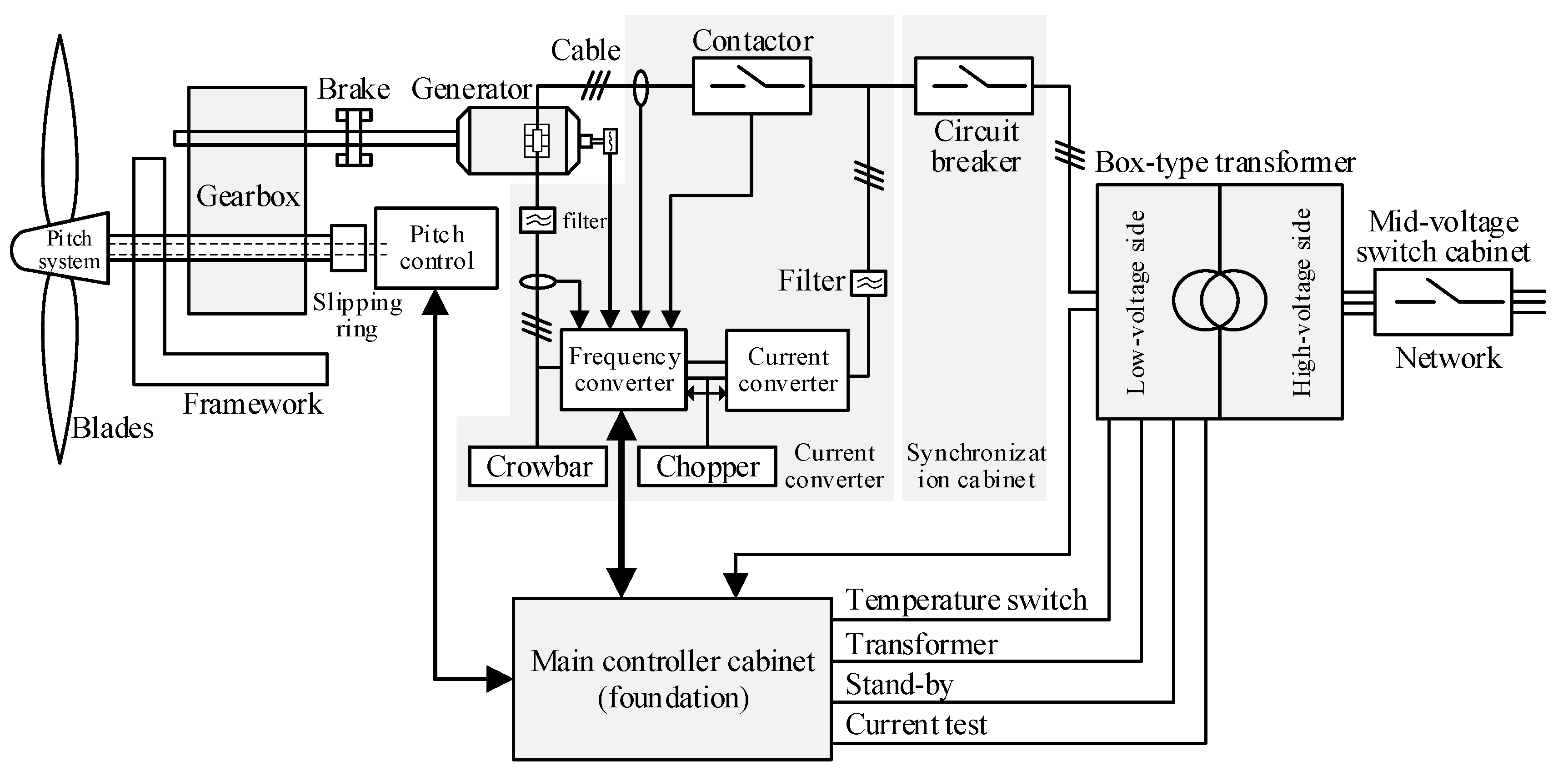
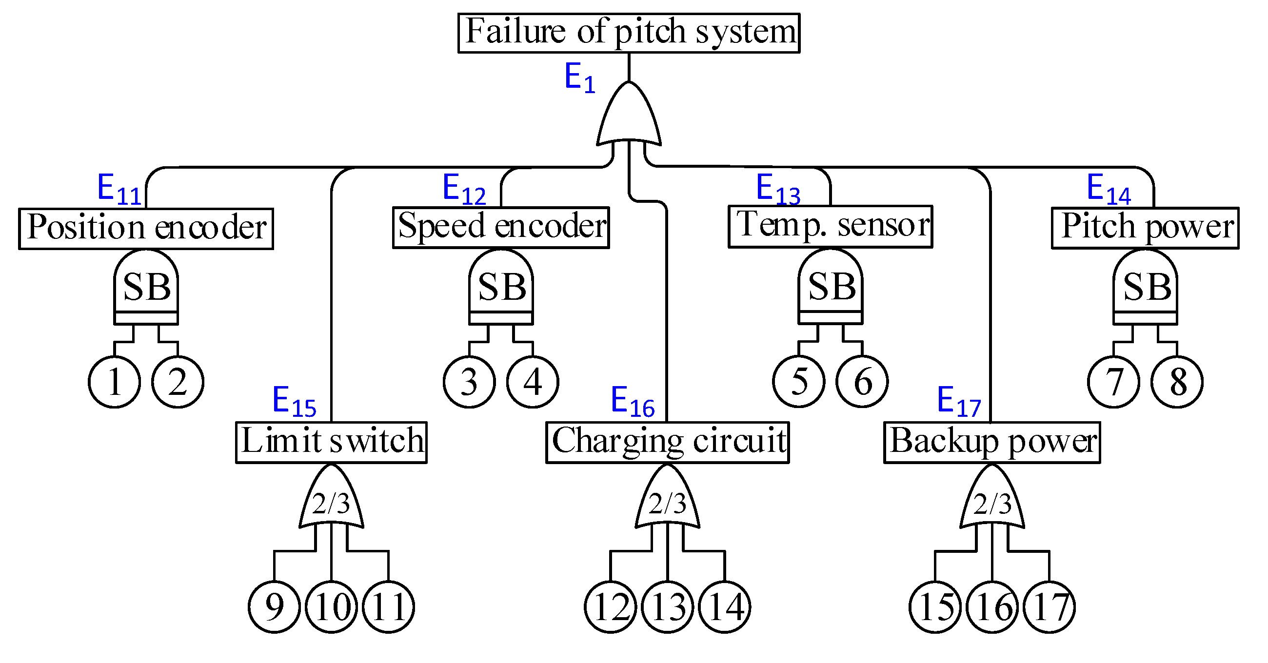
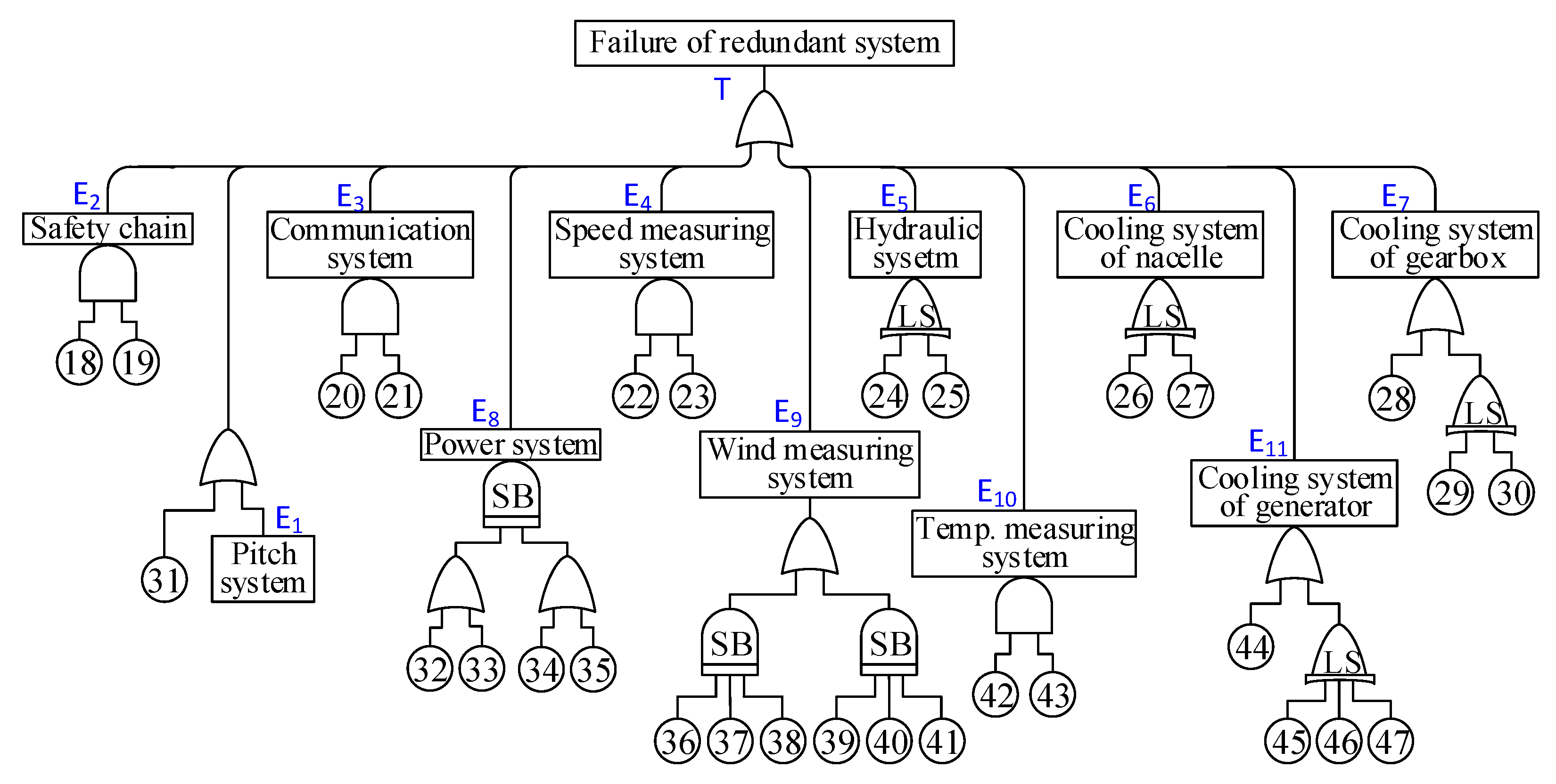
This paper focuses on a 5 MW doubly-fed induction generator with a four-point suspension produced by CSIC (Chongqing) Haizhuang Windpower Equipment Co., Ltd. from Chongqing, China. The system schematic of the offshore wind turbine (OWT) is presented in Figure 1. The OWT is a typical three-bladed, upwind, variable-speed, variable blade-pitch-to-feather-controlled turbine. The rated wind speed and the rated rotor speed are 12.6 m/s and 11.34 rpm, respectively. The design life of the OWT is 20 years. In Figure 1, the entire system of the OWT is a closed-loop control system, and every subsystem is closely related to the others. From the wind turbine structure and the design aspects, it can be seen that redundant systems of OWTs contain multiple types of functional redundancy including parallel redundancy (active redundancy), load-sharing redundancy (partially loaded redundancy), standby redundancy (passive redundancy), and k-out-of-n redundancy (change over redundancy) and redundancy designs exist in eleven subsystems: the pitch system (E1), the safety chain (E2), the communication system (E3), the speed measuring system (E4), the hydraulic system (E5), the cooling system of the nacelle (E6), the cooling system of the gearbox (E7), the power generation system (E8), the wind measuring system (E9), the temperature measuring system of the nacelle (E10), and the cooling system of the generator (E11), which are transformed into the fault tree (FT) of redundant systems shown in Figure 2 and Figure 3.

Figure 1.
System schematic of offshore wind turbine.
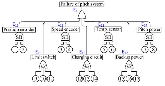
Figure 2.
Fault tree of the pitch system.
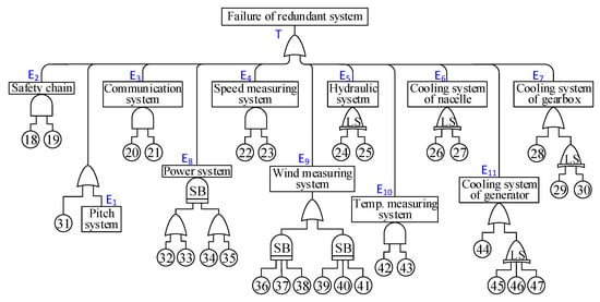
Figure 3.
Fault tree of the redundant system.
As it is shown in Figure 2 and Figure 3, there are five types of gates in the FT of redundant subsystems: AND gate, OR gate, Voting OR gate, Standby gate, and Load Sharing gate. The AND and OR gates are the most basic types of gates in classical fault tree analysis. The basic symbolic descriptions are shown in Table 1. The logic symbol of k-out-of-n redundancy in a fault tree is represented as Voting OR gate in which the output event occurs if k or more of the input events occur (k ≤ n). For standby redundancies, alike E11 and E12, when the active component fails, the “standby” backup component will take over the role of the failed component by the switch and the original system continues to function. Standby redundancy is one of the most commonly used redundancy methods in WTs. To illustrate the failure mechanism of load-sharing redundancy, the concept of load sharing in the field of WTs is proposed [21]. It is should be noted that components of the load-sharing redundancy will share a full load if both of them function, and the surviving component will suffer the full load if one component fails. In the OWT, the hydraulic system (E5), the cooling system of the nacelle (E6), the cooling system of the gearbox (E7) and the cooling system of the generator (E11) belong to load-sharing subsystems.

Table 1.
The symbolic descriptions.
The specific information of basic events is depicted in Table 2 including components’ name, type of redundancy, mean time between failure (MTBF) and distribution type of failure times. The data of components’ MTBF is real maintenance records provided by CSIC (Chongqing) Haizhuang Windpower Equipment Co., Ltd. Because reliability data of components can not be used directly, it needs to transform them into distribution parameters. Generally, the lifetime of electronic components follows an Exponential distribution with parameter λ, and the lifetime of mechanical components follows a Weibull distribution with scale parameter (λ) and shape parameter (γ) [1,22]. Therefore, the failure rates of electronic components can be calculated by , and the scale parameter of a Weibull distribution can be obtained from MTBF of components using the method proposed in Ref. [21].

Table 2.
Parameters of basic events of fault tree.
3. Methodology
With regard to the problems of component swapping within redundant systems, the related methods in this section are proposed to perform the research mentioned in Section 1. Survival signature is adopted to quantify system reliability when redundant components can be swapped upon failure. The reliability importance indexes (MRI and JRI) are calculated using methods in Section 3.2. Following this, the reliability functions of load-sharing redundant systems and standby redundant systems are derived given in Section 3.3 and Section 3.4, respectively.
3.1. Component Swapping in the Original System
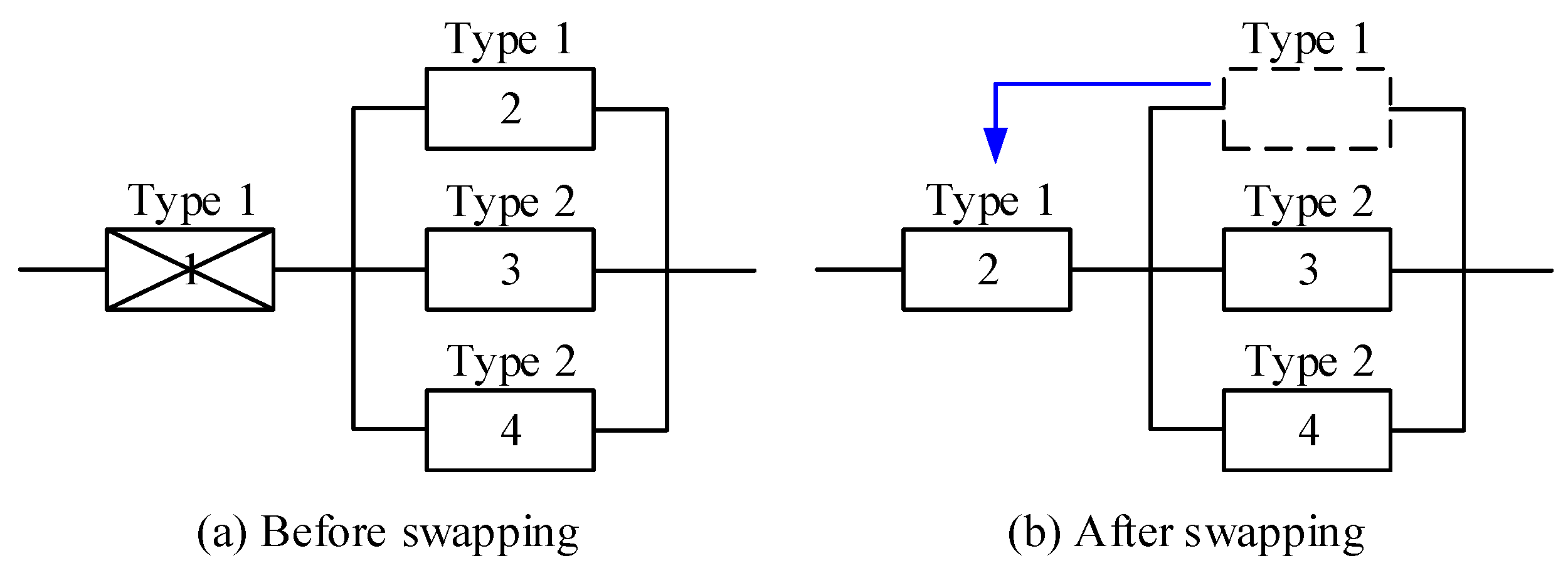
In complex equipment, component redundancy is widely used to improve system reliability, such as parallel redundancy, load-sharing redundancy, standby redundancy and k-out-of-n redundancy. Once systems can not function due to the failures of critical components, shutdowns of entire systems will bring huge economic losses to enterprises. To make failed systems return to work quickly, failed components at a more critical position can be replaced with other functioning components at a less critical position in the original system. As an example, Figure 4 depicts a four-component system of two types. Components 1 and 2 are of the same Type 1, and components 3 and 4 are of the same Type 2. Component 1 is in a more important position than other components, and failure of component 1 will cause the failure of the entire system. Therefore, the system reliability will be improved a lot if component 1 fails and can be replaced by component 2 or components of the same type in the original system.

Figure 4.
Illustration of component swapping.
Survival signature-based component swapping is the possibility to replace a failed component by another component in the system which has not yet failed [11,19]. For a coherent system that consists of m units of types, with units of type and . Let () denote the probability that the system functions. If we assume that there are exactly l units functioning, then the remaining units do not function. is the state vector of units of type k, with if the kth units of type k function and if not. The state vector is introduced to represent the states of units of the type k (). The system’s survival function is represented by that means the probability that the system functions in the condition that exactly of type k units function, for . For the system shown in Figure 4, the survival signature of the original system without swapping , and the system with swapping are presented in Table 3. It can be noted that the values of and are changed from 1/2 to 1, which means the increase in the probability of system’s reliability.

Table 3.
Survival signature of the system in Figure 4 with and without swapping.
Using the failure times of components of different types and cumulative distribution function (CDF) , the system’s reliability can be calculated by
For a situation that some components can be swapped upon the failure of a component, the system structure function given the defined swap in place is represented as . Two swapping rules are made in this study: (i) once a component fails another good component will take over its role in the system; (ii) swaps of components take neglectable time and do not affect the functioning of the component that changes its role in the system nor its remaining useful life [19]. Therefore, the survival signature given the defined swapping regime in place can be expressed as follows
Then the system reliability with the specified swapping regime in place can be obtained as follows
where all swapping strategies are reflected in the survival signature, and effects of component swapping on the system can be seen from the structure function.
The improvement of system reliability due to the swapping regime compared to the situation without swaps is given from Equations (1) and (3)
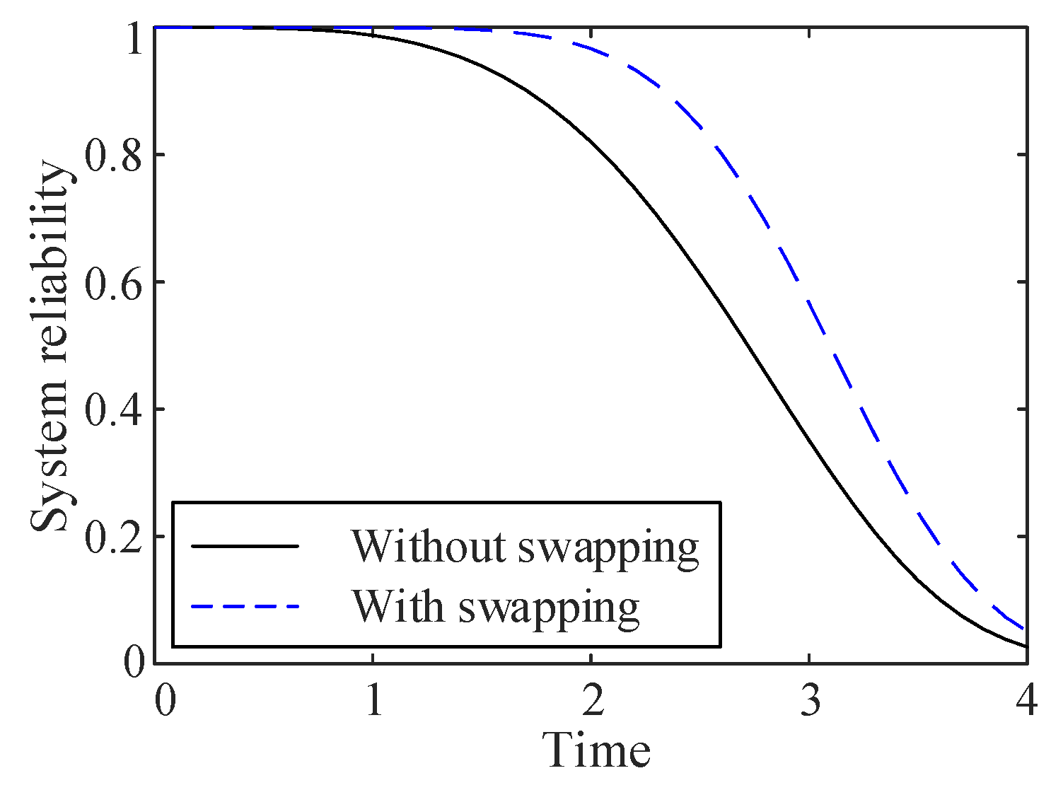
The example shown in Figure 4 is used to illustrate the effects of component swapping on system reliability. Let CDFs of components of each type be and , and the system reliability curves with and without swapping are shown in Figure 5. The results of this figure clearly present that component swapping can greatly improve the reliability of the entire system.
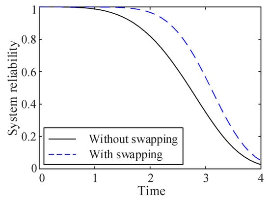
Figure 5.
Reliability curves of the system considering swapping.
3.2. Reliability Importance Measure Of Components
3.2.1. Analytical Method for the Imprecision of Components MTBF
In engineering practice, the probabilistic behavior of complex equipment can not be fully characterized due to the uncertainties of working conditions. This problem can be tackled by implementing probabilistic methods, alike imprecise probability method [23]. Coolen et al. developed a nonparametric predictive inference (NPI) based imprecise reliability analysis method using survival signature [10]. In fact, global optimization procedures are adopted to obtain lower and upper bounds for a complex system with multiple fuzzy variables [24,25].
Assume lower distribution functions and upper distribution functions are nondecreasing functions mapping the real line into [0,1] and for all real values x [26]. According to the framework of a p-box [27], the lower and upper bounds of CDFs of the failure times of type k component can be represented as and , respectively. Let be intervals of type k component. The kth value of the reliability function is also an interval.
Coolen et al. presented nonparametric predictive inference (NPI) for system reliability using survival signature in [10]. This approach can be used to calculate the lower and upper bounds of the survival function for a system with K types of components. For , let denote the number of components of type k and let represent the number of components of type k that function at time t. This study assumes that the failure ends the functioning of a component and it can not be repaired or replaced. Therefore, the lower and upper bounds of the survival function can be expressed as follows
where
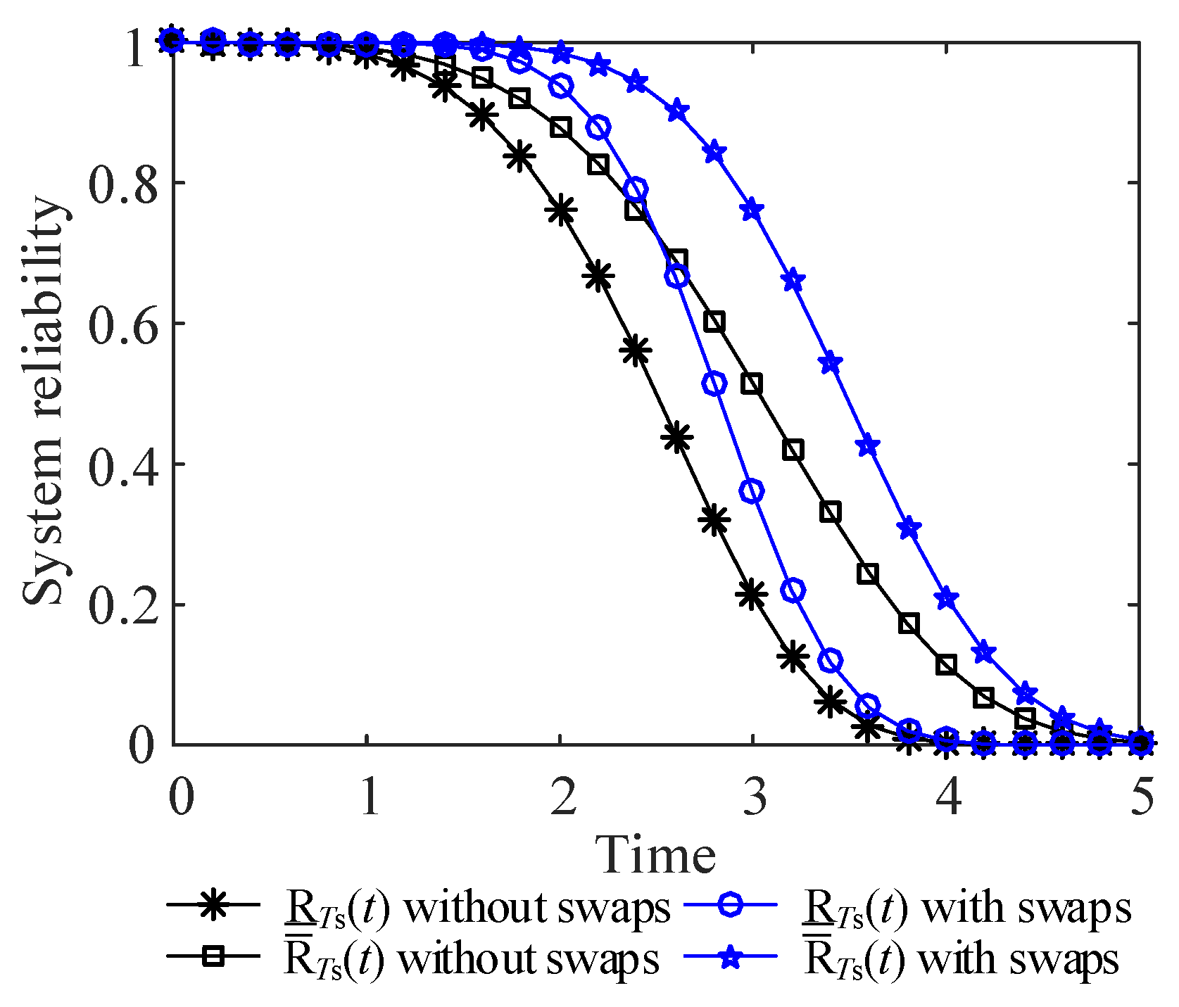
Taking the system presented in Figure 4 as example, let scale parameters of components be uncertain ( for type 1 and for type 2). Hence, it is known that , , , and . The lower and upper bounds of system reliability function become
Hence, the lower and upper bounds of system reliability of the example can be obtained using Equations (7), which are shown in Figure 6.
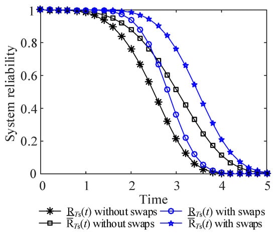
Figure 6.
Lower and upper bounds of system reliability considering swapping.
3.2.2. Component Reliability Importance
In this paper, the reliability importance considering component swapping with the imprecise probabilities are combined to explore the uncertainties of failure times on the reliability importance of a component. For a single component i of type k, the reliability importance is the difference between the probability that the system functions at time t given that component i functions at time t, and the probability that the system functions at time t given that component i does not function at time t [15]. Therefore, the marginal reliability importance (MRI) of component i at time t considering component swapping can be defined as
where and are conditional survival functions that can be easily calculated by the corresponding survival signature.
The imprecise reliability importance with considerations of the uncertainties of failure times is studied. The imprecise failure probabilities of components are represented as distributional p-boxes indicated with = . Therefore, the lower and upper bounds of marginal reliability importance can be calculated by
where
3.2.3. Joint Reliability Importance
A new joint reliability importance measure is presented herein that is expressed as JRI. For s-independent components, the JRI of two components i and j can be defined as
where is the system reliability at time t, and represents the system reliability with component i working and component j failed. If component i and j are of same type k, Equation (12) can be written as follows
where
Generally, for a system with n independent components (), the JRI can be derived as
where the sign before each function h follows the principles: (i) while number n is odd, the sign before the function h is positive if the number of corresponding 1’s is odd, otherwise, it is negative; (ii) while number n is even, the sign before the function h is positive if the number of corresponding 1’s is even, otherwise, it is negative; (iii) the sign of last term is negative if n is odd, otherwise, it is positive [14].
The JRI is introduced to quantitatively measure the interaction of multiple components in a system in contributing to system reliability. For any n components, JRI, and in particular: (a) JRI > 0 indicates that one component becomes more important when the other is functioning (“complements”); (b) JRI < 0 indicates that one component becomes less important when the other is functioning (“substitutes”); (c) JRI = 0 indicates that one component’s importance is unchanged by the functioning of the other [13].
3.3. Reliability of Load-Sharing Redundancy
The concept of load sharing was proposed to deal with the problem that most redundant components are treated as parallel redundancy, which is not true in reality [21]. The quantification of the system reliability of redundant components is determined based on the assumption that when one redundant component fails, the failure rates of other components do not change during the mission. However, this assumption is not correct in engineering practice. The remaining components will suffer higher failure rates due to the increased share of the load during the mission, which will reduce the system’s reliability.
Considering a two-component load-sharing system, it is reasonable to assume that the lifetime of components follows a two-parameter Weibull distribution with scale parameter () and shape parameter (). The state transition diagram the system is depicted in Figure 7. The system reliability function () can be derived as follows.

Figure 7.
Load-sharing with two redundant components .
The first term of Equation (16) is the probability that component 1 and 2 complete their mission from 0 to t successfully with pdf’s and , respectively. It can be expressed as
The second term of Equation (16) is the probability that component 1 fails at with pdf, and component 2 functions until with pdf and then functions for the rest of the mission with pdf. The second term of Equation (16) can be written as follows
The third term of Equation (16) can also be obtained in the same way, as follows:
3.4. Reliability of Standby Redundancy
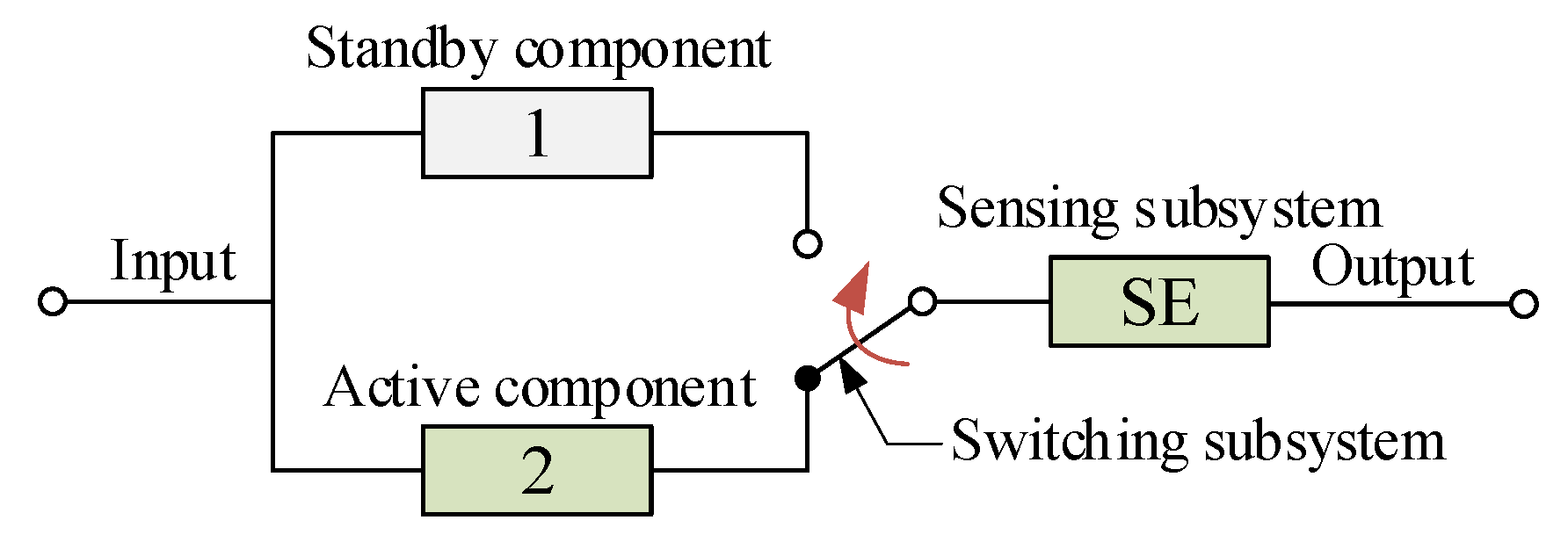
A two-component standby system succeeds in two conditions: (1) when the active component, the sensing subsystem and the switch do not fail; (2) the active component fails before the end of the mission, the sensing and switching subsystems do not fail, and the standby component not having already failed succeeds for the remainder of the mission. The reliability block diagram of such a standby system is given in Figure 8.
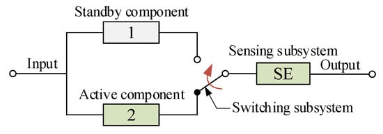
Figure 8.
Two-unit standby system with sensing and switching subsystems.
Assuming that the failures of different components and the failures due to different failure modes are independent, the probability of the first condition is expressed mathematically by
where is the reliability of component 1 in the energized mode at time t during the whole mission, means the reliability of the sensing subsystem at time t, and represents the switch does not fail open from 0 to t.
For the second condition, component 1 fails in a time interval () before time t, and the sensing subsystem does not fail by . The switching subsystem functions in the quiescent mode by , and the switch successfully switches in the standby component in the energized mode with a one-cycle operation, at which time the standby component does not fail by in quiescent mode. Following this, the standby component will function successfully for the remainder of the mission in the energized mode. The switch does not fail open until the end of the mission. Therefore, the probability of the second condition can be derived as follows
where is a variable quantity ().
Assuming that all components have constant failure rates and the lifetime of each component follows an Exponential distribution. From the formula , taking the natural logarithm of both sides of Equation , the equivalent time can be obtained. Finally, the reliability of standby systems can be expressed as
In addition, for a standby system with n identical components where one component is functioning and components are in standby, the reliability of the standby system can be calculated by
where is the number of components that fail.
If the lifetime of components in a standby system follows a two-parameter Weibull distribution with parameters and , the equivalent time and the ith component reliability can be obtained. The reliability formula of the standby system can also be derived by the proposed method from Equations (20) and (21)
where and represent scale parameters and shape parameters of component i (i = 1, SE, SWO, SWQ, SWE, 2Q and 2E).
4. Reliability Analysis of Redundant Systems
In this section, a survival signature-based system reliability model is established for the OWT. Reliability analysis of the entire system with considerations of components swapping is conducted. Calculations of multiple swapping cases are performed to explore the effects of component swapping of different types on the system reliability.
The reliability block diagram of swapping components of three types is given in Figure 9. Considering the subsystem in Figure 9, which has twelve components of three types (K = 3), components 5, 6, 28, 31, 42, 43 and 44 are of type 1 (), components 29, 45 and 46 are of type 2 (), and components 30 and 47 are of type 3 (). Four swapping cases of the OWT system are defined. The case without swapping is treated as case 0. In case 1, all components of three types can be swapped, and swapping can only happen among the same type components. In cases 2, 3 and 4, only components of type 1, type 2, and type 3 can be swapped when needed to keep the system functioning, respectively. It is very time-consuming and difficult to calculate the survival signature of all cases. For this reason, an R package created by Aslett is used to obtain the survival signature of each case in this study [28]. The survival signature of the subsystem with swapping components is derived and presented in Table 4, where , , , and represent structure functions of Case 0, Case 1, Case 2, Case 3, and Case 4, respectively.

Figure 9.
Reliability block diagram of swapping components.

Table 4.
Survival signature of the system in Figure 9 (rows with are omitted).
According to the approaches proposed in Section 3.1, the reliability function of the subsystem shown in Figure 9 with component swapping is derived as follows
where i = 0, 1, 2, 3 and 4.
For load-sharing redundancy subsystems, alike events and , the corresponding reliability function can be obtained from Equation (16)
where , and are scale and shape parameters of components taking full loads, respectively, and and represent scale and shape parameters of components taking sharing loads, respectively ().
For standby redundancy subsystems, alike events , , the corresponding reliability function can be obtained from Equations (22) and (24)
where and represent scale parameters and shape parameters of component i (i = 1, SE, 2Q and 2E).
Considering redundancy subsystems, the system reliability is equal to the probability that the number of working components is greater than or equal to 2, which can be expressed as follows
where is the reliability of components of subsystem at time t ().
According to the FT of redundant systems shown in Figure 2 and Figure 3, the minimal cut set of subsystems can obtained as follows:
T:
E1:
Therefore, the reliability of the redundant system of OWT can be obtained by
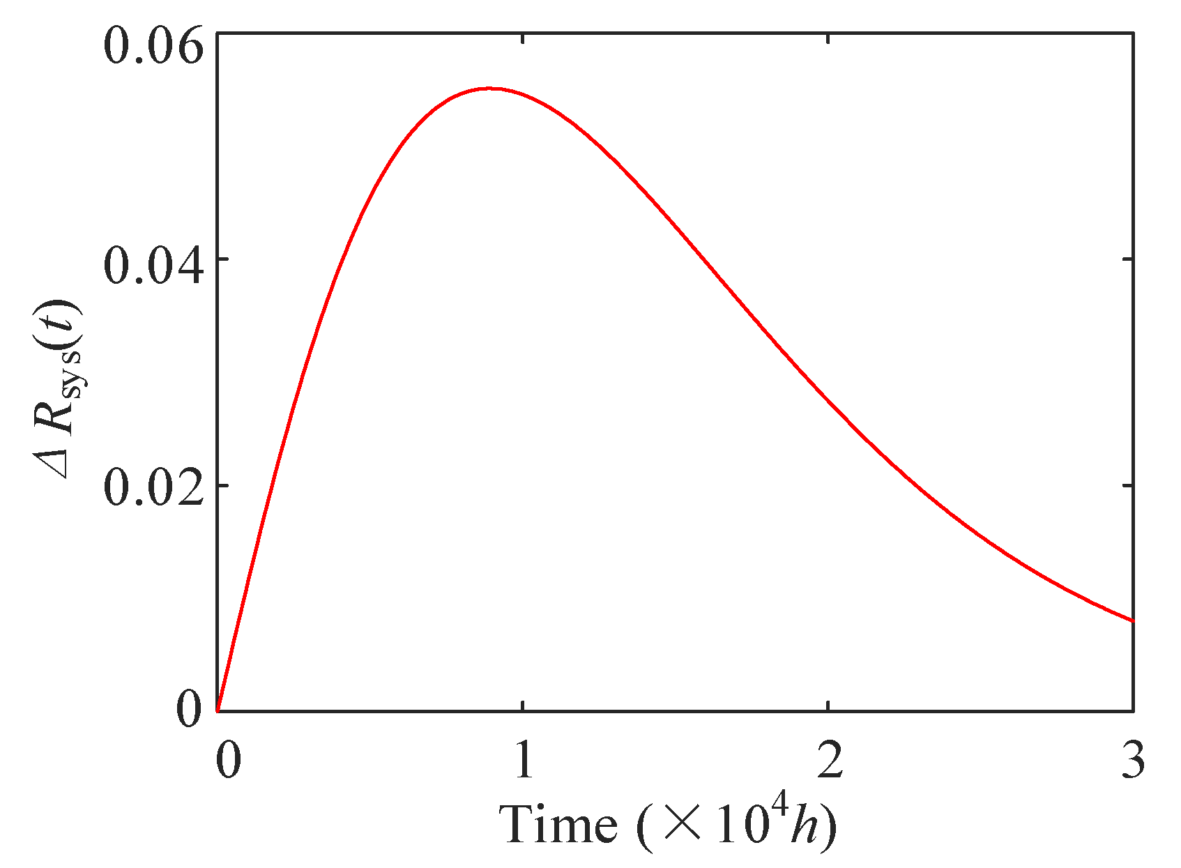
Using the methods given above, the time-dependent reliability of redundant systems in Figure 3 can be obtained, and the reliability curves are shown in Figure 10. As it is shown in Figure 10, the dotted line and the solid line represent system reliability with and without considerations of component swapping, respectively. The system reliability considering component swapping is significantly larger than that of the system without swapping. To measure the increase of system reliability, a function that is the difference of system reliability between two situations is defined. Figure 11 presents the absolute increase in system reliability at a given time t. It can be seen from Figure 11 that the absolute increase of system reliability () is increasing with the increase of time t ( h), and the absolute increase of system reliability will decrease when time h. Therefore, the component swapping makes the greatest contribution to the reliability improvement of redundant systems of offshore wind turbine at h, which means that the “optimal” performance will be obtained if swapping failed components is performed at time h.
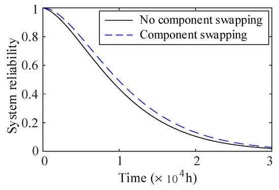
Figure 10.
System reliability with all possible swapping.
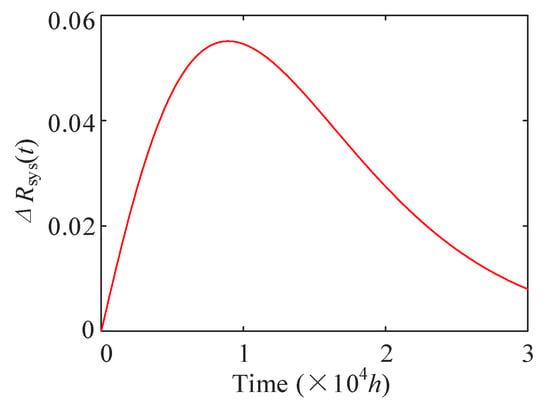
Figure 11.
Improvement of system reliability with component swapping.
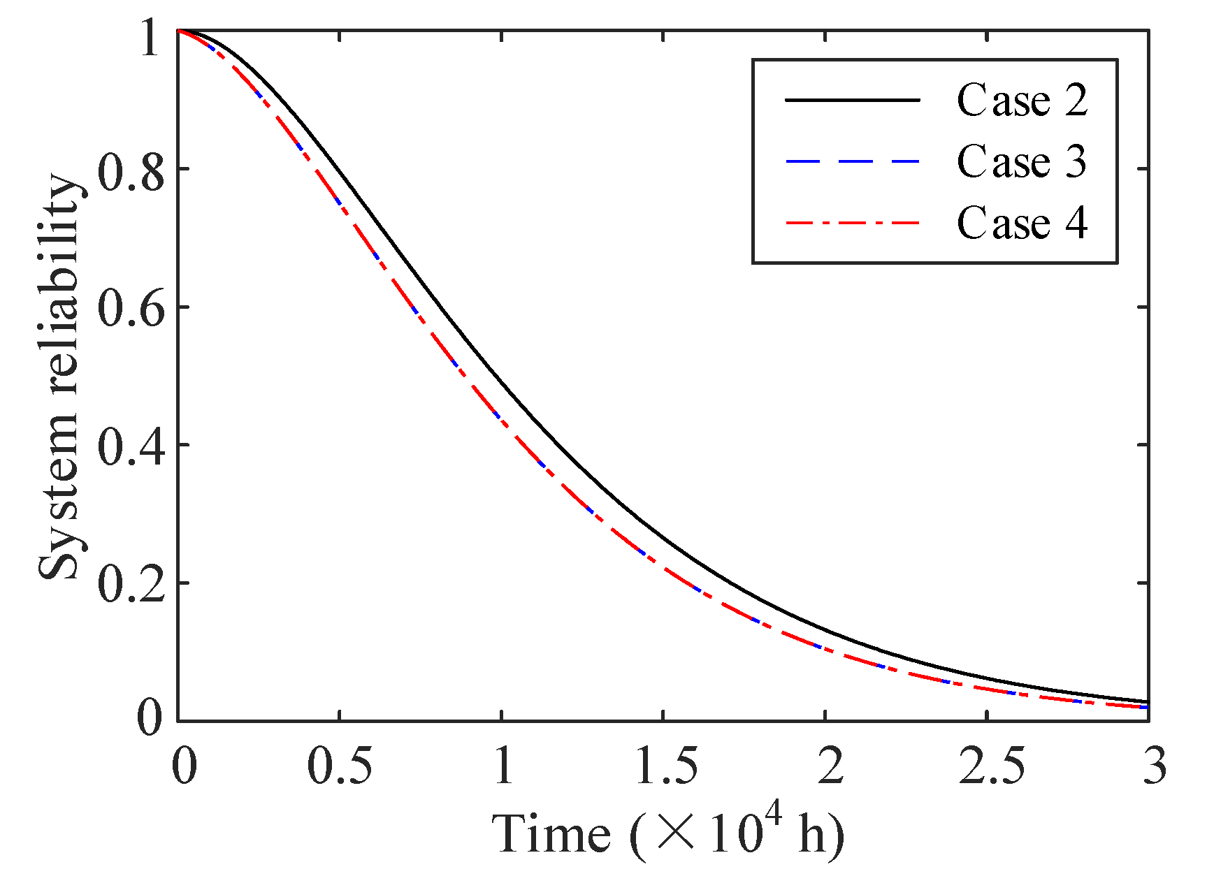
Besides, to examine the system reliability with different swapping components, three swapping cases are compared. In case 2, only Type 1 components are able to be swapped, in case 3, only Type 2 components can be swapped, and in case 4, only Type 3 components can be swapped. The system reliability curves are given in Figure 12. Clearly, Case 2 provides the best improvement of system reliability than others, which is mainly because Type 1 components are at critical locations in the original system, and the effects of component swapping of Case 3 and 4 on system reliability are the same. Because the levels of redundancy of Type 2 and 3 components are similar. Therefore, the positions of temperature sensors of Type 1 are more important than that of the cooling fan of Type 2 and the cooling pump of Type 3. The positions of temperature sensors should be paid more attention and be allocated more resources (inspections, spare components, etc.) than other components.
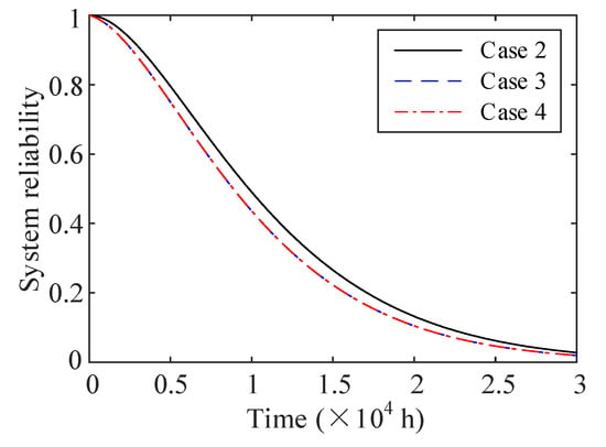
Figure 12.
System reliability with different swapping strategies.
5. Component Reliability Importance
For critical components that can be swapped, the reliability importance of a specific component or multiple components needs to be measured in the way described in Section 3.2. Components are defined based on their locations in the original system. The results of reliability importance analysis can help rank critical components, and allocate more resources (reliability and maintenance) to weakness than others.
5.1. Marginal Reliability Importance
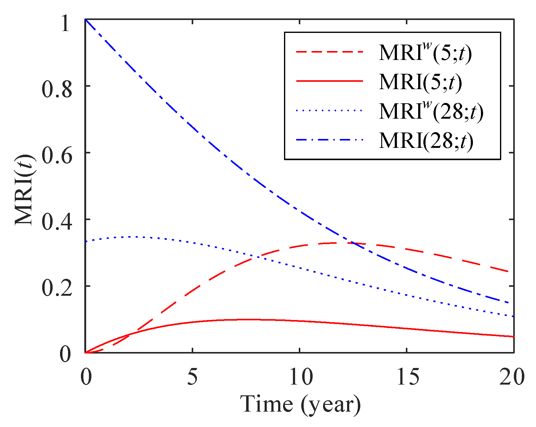
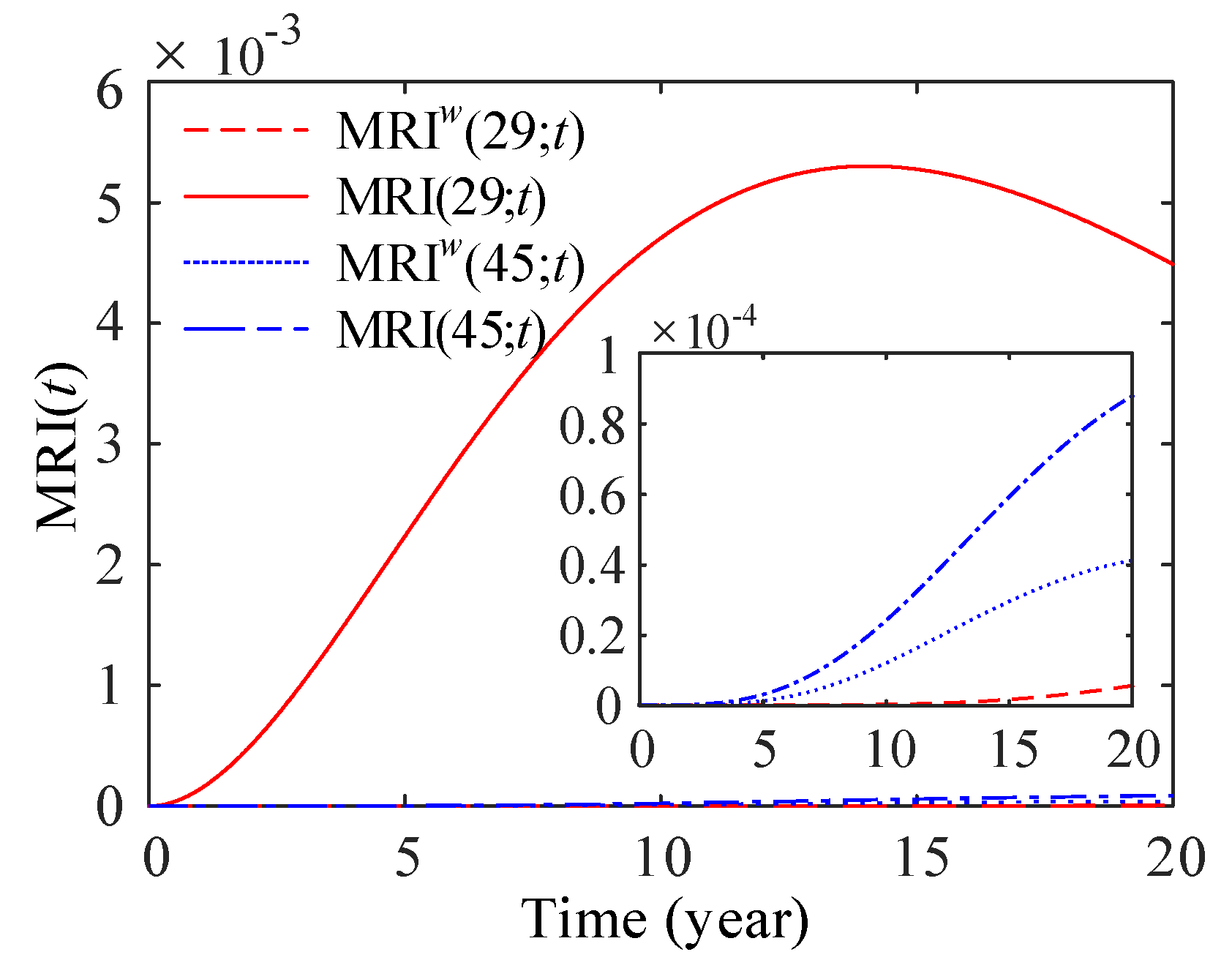
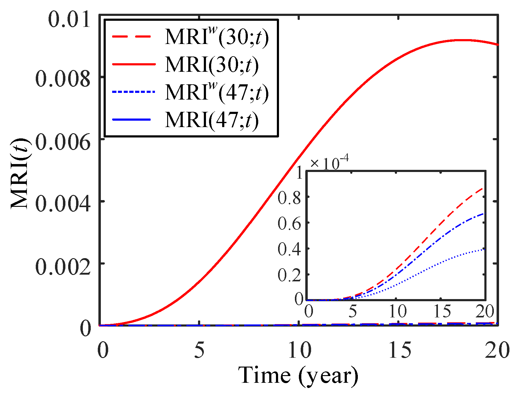
For the system shown in Figure 9, there are multiple components of the same type in the same location. In this study, components 5 and 28 of Type 1, components 29 and 45 of Type 2, and components 30 and 47 of Type 3 are taken as research objects. The and of each component without and with swapping are given in Table A1, Table A2 and Table A3 in Appendix A. MRI analysis of components 5, 28, 29, 45, 30, and 47 with and without swapping is performed, the results of which are shown in Figure 13, Figure 14 and Figure 15. The findings show that MRIs of components 5 and 28 of Type 1 are much larger than that of components 29, 45 of Type 2 and components 30 and 47 of Type 3 by comparisons of three figures. In Figure 13, the MRI of component 5 considering component swapping (MRI is larger than that of component 5 without considering component swapping (MRI), which means that considering component swapping can increase the MRI of component 5. The MRI of component 28 considering component swapping (MRI) is much less than that of component 28 without considering component swapping (MRI), which indicates that component swapping can reduce the MRI of component 28.
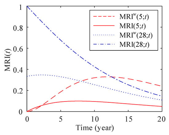
Figure 13.
MRI of components (5 and 28) with and without swapping.

Figure 14.
MRI of components (29 and 45) with and without swapping.
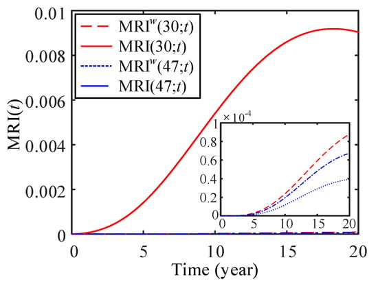
Figure 15.
MRI of components (30 and 47) with and without swapping.
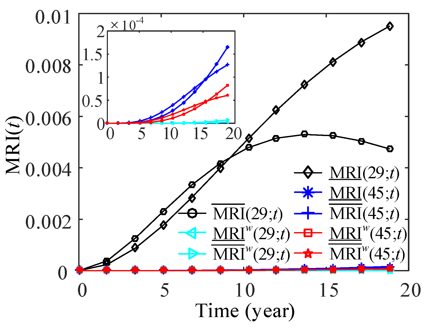
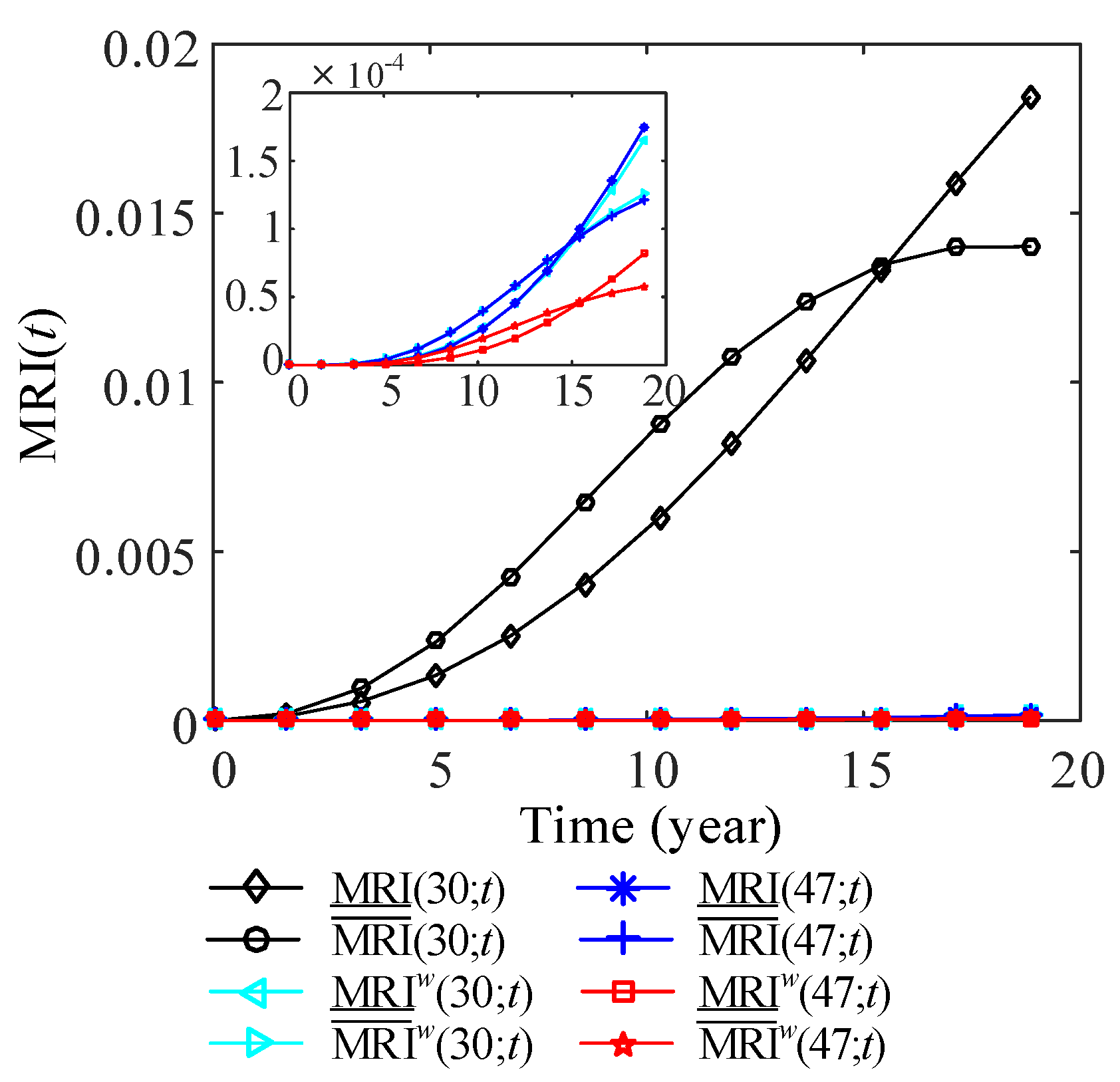
The results of Figure 14 show that the MRI of component 29 without considering component swapping (MRI) is much larger than that of the rest cases. In the inner figure of Figure 14, the MRI of component 45 without swapping (MRI) is the largest than other cases, and the MRIs of components 45 and 29 with swapping (MRI and MRI) are second and third. Therefore, considering component swapping can reduce the MRI of components 29 and 45 of Type 2. The same results also occur for components 30 and 47. As shown in Figure 15, the MRI of component 30 without swapping (MRI) is the largest than other cases, and the MRI of component 30 with swapping (MRI)) is larger than that of component 47 without and with swapping (MRI and MRI). Component swapping can significantly reduce the MRI of components 30 and 47 of Type 3.
The failure rates of swapping components are uncertain due to different working conditions and random loads. In addition, manufacturers of wind turbines like to apply components from different manufacturers in wind turbines to evaluate their reliability levels and reduce the investment risk. In this paper, the influences of uncertainties of failure rates on the MRI of swapping components are explored. Let the MTBF of Type 1 components be in a interval h, MTBF of Type 2 components be in a interval h, and MTBF of Type 3 components be in a interval h. The lower and upper bounds of components MTBF reflect the best and the worst performance of the components, respectively. Using the proposed method in Section 3.2, lower and upper MRI of each swapping components can be obtained. Figure 16 presents the lower and upper MRI of components 5 and 28 with and without considering component swapping. The imprecision of components’ MTBF is translated into the imprecision of MRI of components 5 and 28. The imprecision of components’ MTBF greatly affects the MRI of component 28. Lower and upper MRI of components 29 and 45 of Type 2, and components 30 and 47 of Type 3 are given in Figure 17 and Figure 18, respectively. It can be seen from the figures that the uncertainties of components’ MRI are increasing with the increase of time t. Moreover, the MRI of components without swapping is still larger than that of components with swapping.
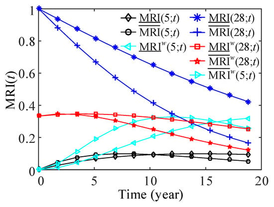
Figure 16.
Lower and upper MRI of components 5 and 28.

Figure 17.
Lower and upper MRI of components 29 and 45.
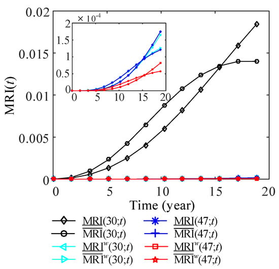
Figure 18.
Lower and upper MRI of components 30 and 47.
5.2. Joint Reliability Importance
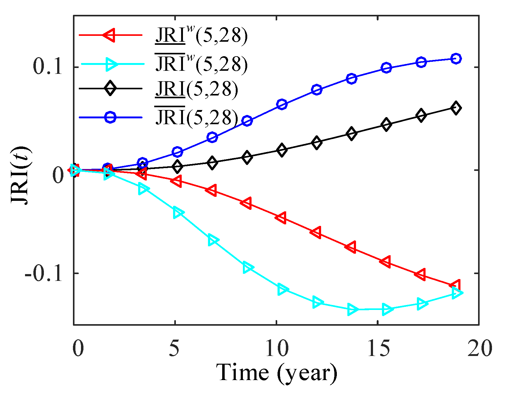
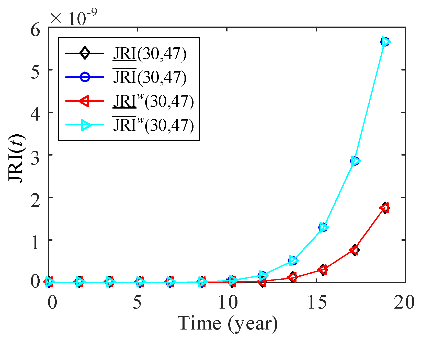
Since components of the same type are dependent, it is necessary to perform the JRI analysis of multiple components with and without considerations of component swapping. Survival signatures of given states of components are shown in Table A4, Table A5 and Table A6 in Appendix A. The lower and upper JRI of components 5 and 28 of Type 1, components 29 and 45 of Type 2 and components 30 and 47 of Type 3 are shown in Figure 19, Figure 20 and Figure 21, respectively. The results show that the fuzzy failure rates cause the uncertainties of JRI of two components. The influences of imprecise failure rates on the JRI of components 5 and 28 is larger than that of components 29 and 45, and components 30 and 47. In Figure 19, the JRI of components 5 and 28 with considerations of components swapping is less than zero, which means that one component becomes less important while the other component is functioning (“substitutes”) [19]. However, the MRI of components 5 and 28 without swapping ( and ) is greater than zero. The relationship between components 5 and 28 is changed from “complements” to “substitutes” if component swapping is considered. For the cases that the JRI of components is greater than zero in Figure 20 and Figure 21, one component becomes more important while the other component is functioning (“complements”). The results of Figure 20 indicate that imprecise failure rates have little effects on the JRI of components 29 and 45 without swapping ( and ). The JRI of components 30 and 47 with and without swapping are the same. This is because only two components of Type 3 are available, and the structure function of the system in Figure 9 without and with swapping does not change.
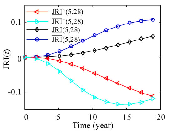
Figure 19.
Lower and upper JRI of components 5 and 28.
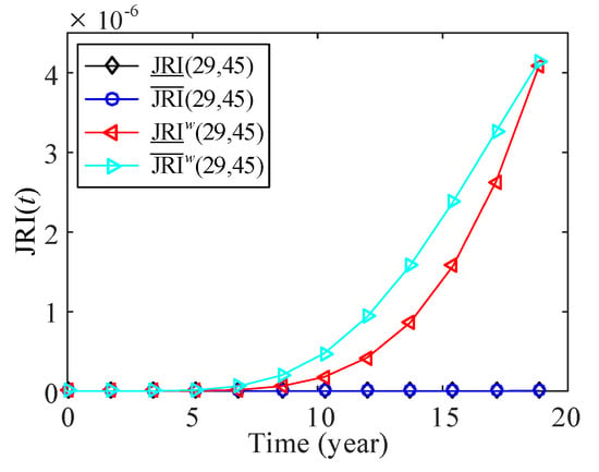
Figure 20.
Lower and upper JRI of components 29 and 45.
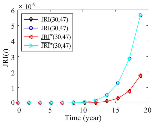
Figure 21.
Lower and upper JRI of components 30 and 47.
6. Conclusions
In this paper, the reliability of redundant systems of offshore wind turbines considering component swapping is assessed. Survival signature-based component swapping is introduced to express the new structure-function of redundant systems after swapping. FT based reliability model considering component swapping is proposed to obtain the realistic reliability assessment of redundant systems. Moreover, both marginal reliability importance index and joint reliability importance index of critical components with and without swapping are calculated to explore the influences of component swapping on component reliability importance and rank the importance of individual components. The effects of the imprecision of failure rates on component reliability importance are also studied.
Considering component swapping can significantly improve system reliability, which is shown in Figure 10. Furthermore, as shown in Figure 11, the improvement of system reliability is increasing first and then decreasing with the increase of time t. The obtains the maximum value (0.0551) at time h. The influences of different swapping components on system reliability are explored, and the findings show that swapping components of Type 1 (the temperature sensor) is the “best” option of swapping strategies, which means that the location of components of Type 1 is more important than that of other types (the cooling fan and the cooling pump). Therefore, components of Type 1 should be allocated more resources for repair, maintenance and inspection than other components.
To quantify the importance degree of critical components, the marginal reliability importance measure and joint reliability importance measure without and with swapping are performed. The findings show that considering component swapping decreases component reliability importance (MRI and JRI). The importance degrees of individual and a couple of components are ranked to help conduct an optimal allocation of resources for operation and maintenance. The ranks of the MRIs of individual components without swapping are MRI(28;t) > MRI(5;t) > MRI(30;t) > MRI(29;t) > MRI(45;t) > MRI(47;t). The ranks of the JRIs of components without and with swapping are the same JRI) > JRI) > JRI). The lower and upper bounds of MRI and JRI of components at a given time t are obtained. The results indicate that the proposed method is a practical and efficient method to perform reliability analysis of redundant systems considering component swapping and examine component reliability importance.
In future work, we intend to establish a reliability optimization model considering constraints of the number, cost, weight, and volume of redundant components and explore the optimal swapping strategy for the improvement of system reliability of offshore wind turbines.
Author Contributions
Conceptualization, Y.L.; methodology, Y.L. and C.Z.; software, C.Z.; validation, Z.W. and Y.L.; formal analysis, C.Z.; investigation, Y.L.; resources, C.Z.; data curation, Z.W.; writing—original draft preparation, Y.L.; writing—review and editing, C.Z.; visualization, Z.W.; supervision, C.Z.; project administration, C.Z.; funding acquisition, C.Z. All authors have read and agreed to the published version of the manuscript.
Funding
This research was funded by the National Key R&D Program of China (Grant No. 2018YFB1501300), Chongqing Innovation and Application Program (Grant No. cstc2019jscx-mbdxX0003), and Central University Basic Scientific Research Project of Chongqing University (Grant No. 2019CDCGJX0017).
Conflicts of Interest
The authors declare no conflict of interest.
Abbreviations
The following abbreviations are used in this manuscript:
| SWO | switch does not fail open |
| SWQ | switch does not fail in the quiescent mode |
| SE | sensing subsystem |
| 1E | component 1 in the energized mode |
| SWC | switch does not fail closed |
| SWE | switching subsystem in the energized mode |
| 2Q | component 2 in the quiescent mode |
| 2E | component 2 in the energized mode |
Nomenclature
| pdf of component 1 with parameters and when it carries the load | |
| pdf of component 1 with parameters and when it carries full load L | |
| probability of component 1 fails at time | |
| conditional reliability function of component 1 after component 2 fails at time | |
| MRI | MRI of component i without swapping at time t |
| MRI | MRI of component i with swapping at time t |
| pdf of component 2 with parameters and when it carries the load | |
| pdf of component 2 with parameters and when it carries full load L | |
| probability of component 2 fails at time | |
| conditional reliability function of component 2 after component 1 fails at time | |
| JRI | JRI of components i and j without swapping at time t |
| JRI | JRI of components i and j with swapping at time t |
Appendix A

Table A1.
and for components 5 and 28 without and with swapping (rows with are omitted).
Table A1.
and for components 5 and 28 without and with swapping (rows with are omitted).
| Without Swapping | With Swapping | Without Swapping | With Swapping | |||||||
|---|---|---|---|---|---|---|---|---|---|---|
| 4 | 0 | 2 | 2/15 | 0 | 1 | 0 | 4/15 | 0 | 4/15 | 0 |
| 4 | 1 | 1 | 1/15 | 0 | 1/2 | 0 | 2/15 | 0 | 2/15 | 0 |
| 4 | 1 | 2 | 2/15 | 0 | 1 | 0 | 4/15 | 0 | 4/15 | 0 |
| 4 | 2 | 0 | 4/45 | 0 | 2/3 | 0 | 8/45 | 0 | 8/45 | 0 |
| 4 | 2 | 1 | 5/45 | 0 | 5/6 | 0 | 2/9 | 0 | 2/9 | 0 |
| 4 | 2 | 2 | 2/15 | 0 | 1 | 0 | 4/15 | 0 | 4/15 | 0 |
| 4 | 3 | 0 | 2/15 | 0 | 1 | 0 | 4/15 | 0 | 4/15 | 0 |
| 4 | 3 | 1 | 2/15 | 0 | 1 | 0 | 4/15 | 0 | 4/15 | 0 |
| 4 | 3 | 2 | 2/15 | 0 | 1 | 0 | 4/15 | 0 | 4/15 | 0 |
| 5 | 0 | 2 | 1/2 | 1/3 | 1 | 1 | 2/3 | 0 | 2/3 | 4/15 |
| 5 | 1 | 1 | 1/4 | 1/6 | 1/2 | 1/2 | 1/3 | 0 | 1/3 | 2/15 |
| 5 | 1 | 2 | 1/2 | 1/3 | 1 | 1 | 2/3 | 0 | 2/3 | 4/15 |
| 5 | 2 | 0 | 1/3 | 1/6 | 2/3 | 2/3 | 4/9 | 0 | 4/9 | 8/45 |
| 5 | 2 | 1 | 5/12 | 5/18 | 5/6 | 5/6 | 5/9 | 0 | 5/9 | 2/9 |
| 5 | 2 | 2 | 1/2 | 1/3 | 1 | 1 | 2/3 | 0 | 2/3 | 4/15 |
| 5 | 3 | 0 | 1/2 | 1/3 | 1 | 1 | 2/3 | 0 | 2/3 | 4/15 |
| 5 | 3 | 1 | 1/2 | 1/3 | 1 | 1 | 2/3 | 0 | 2/3 | 4/15 |
| 5 | 3 | 2 | 1/2 | 1/3 | 1 | 1 | 2/3 | 0 | 2/3 | 4/15 |
| 6 | 0 | 2 | 1 | 1 | 1 | 1 | 1 | 0 | 1 | 2/3 |
| 6 | 1 | 1 | 1/2 | 1/2 | 1/2 | 1/2 | 1/2 | 0 | 1/2 | 1/3 |
| 6 | 1 | 2 | 1 | 1 | 1 | 1 | 1 | 0 | 1 | 2/3 |
| 6 | 2 | 0 | 2/3 | 2/3 | 2/3 | 2/3 | 2/3 | 0 | 2/3 | 4/9 |
| 6 | 2 | 1 | 5/6 | 5/6 | 5/6 | 5/6 | 5/6 | 0 | 5/6 | 5/9 |
| 6 | 2 | 2 | 1 | 1 | 1 | 1 | 1 | 0 | 1 | 2/3 |
| 6 | 3 | 0 | 1 | 1 | 1 | 1 | 1 | 0 | 1 | 2/3 |
| 6 | 3 | 1 | 1 | 1 | 1 | 1 | 1 | 0 | 1 | 2/3 |
| 6 | 3 | 2 | 1 | 1 | 1 | 1 | 1 | 0 | 1 | 2/3 |

Table A2.
and for components 29 and 45 without and with swapping (rows with are omitted).
Table A2.
and for components 29 and 45 without and with swapping (rows with are omitted).
| Without Swapping | With Swapping | Without Swapping | With Swapping | |||||||
|---|---|---|---|---|---|---|---|---|---|---|
| 5 | 0 | 1 | 2/21 | 0 | 2/21 | 0 | 2/21 | 0 | 2/21 | 0 |
| 5 | 0 | 2 | 4/21 | 4/21 | 4/21 | 4/21 | 4/21 | 4/21 | 4/21 | 4/21 |
| 5 | 1 | 0 | 4/21 | 0 | 4/21 | 0 | 2/21 | 0 | 2/21 | 0 |
| 5 | 1 | 1 | 4/21 | 2/21 | 4/21 | 4/21 | 1/7 | 2/21 | 1/7 | 1/7 |
| 5 | 1 | 2 | 4/21 | 4/21 | 4/21 | 4/21 | 4/21 | 4/21 | 4/21 | 4/21 |
| 5 | 2 | 0 | 4/21 | 0 | 4/21 | 4/21 | 4/21 | 4/21 | 4/21 | 4/21 |
| 5 | 2 | 1 | 4/21 | 2/21 | 4/21 | 4/21 | 4/21 | 4/21 | 4/21 | 4/21 |
| 5 | 2 | 2 | 4/21 | 4/21 | 4/21 | 4/21 | 4/21 | 4/21 | 4/21 | 4/21 |
| 6 | 0 | 2 | 4/7 | 4/7 | 4/7 | 4/7 | 4/7 | 4/7 | 4/7 | 4/7 |
| 6 | 1 | 1 | 4/7 | 2/7 | 4/7 | 4/7 | 3/7 | 2/7 | 4/7 | 3/7 |
| 6 | 1 | 2 | 4/7 | 4/7 | 4/7 | 4/7 | 4/7 | 4/7 | 4/7 | 4/7 |
| 6 | 2 | 0 | 4/7 | 0 | 4/7 | 4/7 | 4/7 | 4/7 | 4/7 | 4/7 |
| 6 | 2 | 1 | 4/7 | 2/7 | 4/7 | 4/7 | 4/7 | 4/7 | 4/7 | 4/7 |
| 6 | 2 | 2 | 4/7 | 4/7 | 4/7 | 4/7 | 4/7 | 4/7 | 4/7 | 4/7 |
| 7 | 0 | 2 | 1 | 1 | 1 | 1 | 1 | 1 | 1 | 1 |
| 7 | 1 | 1 | 1 | 1/2 | 1 | 1 | 3/4 | 1/2 | 3/4 | 3/4 |
| 7 | 1 | 2 | 1 | 1 | 1 | 1 | 1 | 1 | 1 | 1 |
| 7 | 2 | 0 | 1 | 0 | 1 | 1 | 1 | 1 | 1 | 1 |
| 7 | 2 | 1 | 1 | 1/2 | 1 | 1 | 1 | 1 | 1 | 1 |
| 7 | 2 | 2 | 1 | 1 | 1 | 1 | 1 | 1 | 1 | 1 |

Table A3.
and for components 30 and 47 without and with swapping (rows with are omitted).
Table A3.
and for components 30 and 47 without and with swapping (rows with are omitted).
| Without Swapping | With Swapping | Without Swapping | With Swapping | |||||||
|---|---|---|---|---|---|---|---|---|---|---|
| 5 | 1 | 1 | 4/21 | 4/63 | 4/21 | 4/21 | 4/21 | 8/63 | 4/21 | 4/21 |
| 5 | 2 | 0 | 4/21 | 8/63 | 4/21 | 8/63 | 8/63 | 8/63 | 8/63 | 8/63 |
| 5 | 2 | 1 | 1 | 8/63 | 4/21 | 4/21 | 4/21 | 4/21 | 4/21 | 4/21 |
| 5 | 3 | 0 | 4/21 | 4/21 | 4/21 | 4/21 | 4/21 | 4/21 | 4/21 | 4/21 |
| 5 | 3 | 1 | 4/21 | 4/21 | 4/21 | 4/21 | 4/21 | 4/21 | 4/21 | 4/21 |
| 6 | 1 | 1 | 4/7 | 4/21 | 4/7 | 4/7 | 4/7 | 8/21 | 4/7 | 4/7 |
| 6 | 2 | 0 | 4/7 | 8/21 | 4/7 | 8/21 | 4/7 | 8/21 | 4/7 | 8/21 |
| 6 | 2 | 1 | 4/7 | 8/21 | 4/7 | 4/7 | 4/7 | 4/7 | 4/7 | 4/7 |
| 6 | 3 | 0 | 4/7 | 4/7 | 4/7 | 4/7 | 4/7 | 4/7 | 4/7 | 4/7 |
| 6 | 3 | 1 | 4/7 | 4/7 | 4/7 | 4/7 | 4/7 | 4/7 | 4/7 | 4/7 |
| 7 | 1 | 1 | 1 | 1/3 | 1 | 1 | 1 | 2/3 | 1 | 1 |
| 7 | 2 | 0 | 1 | 2/3 | 1 | 2/3 | 2/3 | 2/3 | 2/3 | 2/3 |
| 7 | 2 | 1 | 1 | 2/3 | 1 | 1 | 1 | 1 | 1 | 1 |
| 7 | 3 | 0 | 1 | 1 | 1 | 1 | 1 | 1 | 1 | 1 |
| 7 | 3 | 1 | 1 | 1 | 1 | 1 | 1 | 1 | 1 | 1 |

Table A4.
Survival signatures of given states of components 5 and 28 (rows with are omitted).
Table A4.
Survival signatures of given states of components 5 and 28 (rows with are omitted).
| Without Swapping () | With Swapping () | |||||||||
|---|---|---|---|---|---|---|---|---|---|---|
| 3 | 0 | 2 | 1/5 | 0 | 0 | 0 | 0 | 0 | 0 | 0 |
| 3 | 1 | 1 | 1/10 | 0 | 0 | 0 | 1/10 | 0 | 0 | 0 |
| 3 | 1 | 2 | 1/5 | 0 | 0 | 0 | 1/5 | 0 | 0 | 0 |
| 3 | 2 | 0 | 2/15 | 0 | 0 | 0 | 2/15 | 0 | 0 | 0 |
| 3 | 2 | 1 | 1/6 | 0 | 0 | 0 | 1/6 | 0 | 0 | 0 |
| 3 | 2 | 2 | 1/5 | 0 | 0 | 0 | 1/5 | 0 | 0 | 0 |
| 3 | 3 | 0 | 1/5 | 0 | 0 | 0 | 1/5 | 0 | 0 | 0 |
| 3 | 3 | 1 | 1/5 | 0 | 0 | 0 | 1/5 | 0 | 0 | 0 |
| 3 | 3 | 2 | 1/5 | 0 | 0 | 0 | 1/5 | 0 | 0 | 0 |
| 4 | 0 | 2 | 3/5 | 0 | 2/5 | 0 | 3/5 | 3/5 | 3/5 | 0 |
| 4 | 1 | 1 | 3/10 | 0 | 1/5 | 0 | 3/10 | 1/10 | 3/10 | 0 |
| 4 | 1 | 2 | 3/5 | 0 | 2/5 | 0 | 3/5 | 3/5 | 3/5 | 0 |
| 4 | 2 | 0 | 2/5 | 0 | 4/15 | 0 | 2/5 | 2/5 | 2/5 | 0 |
| 4 | 2 | 1 | 1/2 | 0 | 1/3 | 0 | 1/2 | 1/2 | 1/2 | 0 |
| 4 | 2 | 2 | 3/5 | 0 | 2/5 | 0 | 3/5 | 3/5 | 3/5 | 0 |
| 4 | 3 | 0 | 3/5 | 0 | 2/5 | 0 | 3/5 | 3/5 | 3/5 | 0 |
| 4 | 3 | 1 | 3/5 | 0 | 2/5 | 0 | 3/5 | 3/5 | 3/5 | 0 |
| 4 | 3 | 2 | 3/5 | 0 | 2/5 | 0 | 3/5 | 3/5 | 3/5 | 0 |
| 5 | 0 | 2 | 1 | 0 | 1 | 0 | 1 | 1 | 1 | 1 |
| 5 | 1 | 1 | 1/2 | 0 | 1/2 | 0 | 1/2 | 1/2 | 1/2 | 1/2 |
| 5 | 1 | 2 | 1 | 0 | 1 | 0 | 1 | 1 | 1 | 1 |
| 5 | 2 | 0 | 2/3 | 0 | 2/3 | 0 | 2/3 | 2/3 | 2/3 | 2/3 |
| 5 | 2 | 1 | 5/6 | 0 | 5/6 | 0 | 5/6 | 5/6 | 5/6 | 5/6 |
| 5 | 2 | 2 | 1 | 0 | 1 | 0 | 1 | 1 | 1 | 1 |
| 5 | 3 | 0 | 1 | 0 | 1 | 0 | 1 | 1 | 1 | 1 |
| 5 | 3 | 1 | 1 | 0 | 1 | 0 | 1 | 1 | 1 | 1 |
| 5 | 3 | 2 | 1 | 0 | 1 | 0 | 1 | 1 | 1 | 1 |

Table A5.
Survival signatures of given states of components 29 and 45 (rows with are omitted).
Table A5.
Survival signatures of given states of components 29 and 45 (rows with are omitted).
| Without Swapping () | With Swapping ( | |||||||||
|---|---|---|---|---|---|---|---|---|---|---|
| 5 | 0 | 2 | 4/21 | 4/21 | 4/21 | 4/21 | 4/21 | 4/21 | 4/21 | 4/21 |
| 5 | 1 | 0 | 4/21 | 4/21 | 0 | 0 | 4/21 | 4/21 | 4/21 | 0 |
| 5 | 1 | 1 | 4/21 | 4/21 | 2/21 | 2/21 | 4/21 | 4/21 | 4/21 | 4/21 |
| 5 | 1 | 2 | 4/21 | 4/21 | 4/21 | 4/21 | 4/21 | 4/21 | 4/21 | 4/21 |
| 6 | 0 | 0 | 4/7 | 0 | 0 | 0 | 4/7 | 0 | 0 | 0 |
| 6 | 0 | 1 | 4/7 | 2/7 | 2/7 | 0 | 4/7 | 2/7 | 2/7 | 0 |
| 6 | 0 | 2 | 4/7 | 4/7 | 4/7 | 4/7 | 4/7 | 4/7 | 4/7 | 4/7 |
| 6 | 1 | 0 | 4/7 | 4/7 | 0 | 0 | 4/7 | 4/7 | 4/7 | 0 |
| 6 | 1 | 1 | 4/7 | 4/7 | 2/7 | 2/7 | 4/7 | 4/7 | 2/7 | 4/7 |
| 6 | 1 | 2 | 4/7 | 4/7 | 4/7 | 4/7 | 4/7 | 4/7 | 4/7 | 4/7 |
| 7 | 0 | 0 | 1 | 0 | 0 | 0 | 1 | 0 | 0 | 0 |
| 7 | 0 | 1 | 1 | 1/2 | 1/2 | 0 | 1 | 1/2 | 1/2 | 0 |
| 7 | 0 | 2 | 1 | 1 | 1 | 1 | 1 | 1 | 1 | 1 |
| 7 | 1 | 0 | 1 | 1 | 0 | 0 | 1 | 1 | 1 | 0 |
| 7 | 1 | 1 | 1 | 1 | 1/2 | 1/2 | 1 | 1 | 1 | 1 |
| 7 | 1 | 2 | 1 | 1 | 1 | 1 | 1 | 1 | 1 | 1 |

Table A6.
Survival signatures of given states of components 30 and 47 (rows with are omitted).
Table A6.
Survival signatures of given states of components 30 and 47 (rows with are omitted).
| Without Swapping () | With Swapping () | |||||||||
|---|---|---|---|---|---|---|---|---|---|---|
| 5 | 0 | 0 | 4/21 | 0 | 0 | 0 | 4/21 | 0 | 0 | 0 |
| 5 | 1 | 0 | 4/21 | 8/63 | 4/63 | 0 | 4/21 | 8/63 | 4/63 | 0 |
| 5 | 2 | 0 | 4/21 | 4/21 | 8/63 | 8/63 | 4/21 | 4/21 | 8/63 | 8/63 |
| 5 | 3 | 0 | 4/21 | 4/21 | 4/21 | 4/21 | 4/21 | 4/21 | 4/21 | 4/21 |
| 6 | 0 | 0 | 4/7 | 0 | 0 | 0 | 4/7 | 0 | 0 | 0 |
| 6 | 1 | 0 | 4/7 | 8/21 | 4/21 | 0 | 4/7 | 8/21 | 4/21 | 0 |
| 6 | 2 | 0 | 4/7 | 4/7 | 8/21 | 8/21 | 4/7 | 4/7 | 8/21 | 8/21 |
| 6 | 3 | 0 | 4/7 | 4/7 | 4/7 | 4/7 | 4/7 | 4/7 | 4/7 | 4/7 |
| 7 | 0 | 0 | 1 | 0 | 0 | 0 | 1 | 0 | 0 | 0 |
| 7 | 1 | 0 | 1 | 2/3 | 1/3 | 0 | 1 | 2/3 | 1/3 | 0 |
| 7 | 2 | 0 | 1 | 1 | 2/3 | 2/3 | 1 | 1 | 2/3 | 2/3 |
| 7 | 3 | 0 | 1 | 1 | 1 | 1 | 1 | 1 | 1 | 1 |
References
- Yao, L.; Caichao, Z.; Youchuan, T. Research status and development tendency of wind turbine reliability. J. China Mech. Eng. 2017, 28, 1125–1133. [Google Scholar]
- Robinson, C.; Paramasivam, E.; Taylor, E.; Morrison, A.; Sanderson, E. Study and Development of a Methodology for the Estimation of the Risk and Harm to Persons From Wind Turbines; RR968 Research Report; Health and Safety Executive: London, UK, 2013. [Google Scholar]
- Roozbeh, B.; Sandborn, P. Overview of Wind Turbine Field Failure Databases: A Discussion of the Requirements for an Analysis. In Proceedings of the ASME 2018 Power Conference Collocated with the ASME 2018 12th International Conference on Energy Sustainability and the ASME 2018 Nuclear Forum, Lake Buena Vista, FL, USA, 24–28 June 2018. [Google Scholar]
- Ardakan, M.A.; Hamadani, A.Z. Reliability–redundancy allocation problem with cold-standby redundancy strategy. Simul. Model. Pract. Theory 2014, 42, 107–118. [Google Scholar] [CrossRef]
- Way, K.; Prasad, V.R. An annotated overview of system-reliability optimization. IEEE Trans. Reliab. 2000, 49, 176–187. [Google Scholar]
- DNV GL. Failure Mode and Effect Analysis (FMEA) of Redundant Systems DNV-RP-D102; DET NORSKE VERITAS (DNV): Hamburg, Germany, 2012. [Google Scholar]
- Huang, X.; Coolen, F.P.; Coolen-Maturi, T. A heuristic survival signature based approach for reliability-redundancy allocation. Reliab. Eng. Syst. Saf. 2019, 185, 511–517. [Google Scholar] [CrossRef]
- Xiao, N.C.; Huang, H.Z.; Wang, Z.; Li, Y.; Liu, Y. Reliability analysis of series systems with multiple failure modes under epistemic and aleatory uncertainties. Proc. Inst. Mech. Eng. Part O J. Risk Reliab. 2012, 226, 295–304. [Google Scholar] [CrossRef]
- Patelli, E.; Feng, G.; Coolen, F.P.; Coolen-Maturi, T. Simulation methods for system reliability using the survival signature. Reliab. Eng. Syst. Saf. 2017, 167, 327–337. [Google Scholar] [CrossRef]
- Coolen, F.P.; Coolen-Maturi, T.; Al-Nefaiee, A.H. Nonparametric predictive inference for system reliability using the survival signature. Proc. Inst. Mech. Eng. Part O J. Risk Reliab. 2014, 228, 437–448. [Google Scholar] [CrossRef]
- Coolen, F.P.; Coolen-Maturi, T. Generalizing the signature to systems with multiple types of components. In Complex Systems and Dependability; Springer: Berlin/Heidelberg, Germany, 2013; pp. 115–130. [Google Scholar]
- Hong, J.S.; Lie, C.H. Joint reliability-importance of two edges in an undirected network. IEEE Trans. Reliab. 1993, 42, 17–23. [Google Scholar] [CrossRef]
- Armstrong, M.J. Joint reliability-importance of components. IEEE Trans. Reliab. 1995, 44, 408–412. [Google Scholar] [CrossRef]
- Gao, X.; Cui, L.; Li, J. Analysis for joint importance of components in a coherent system. Eur. J. Oper. Res. 2007, 182, 282–299. [Google Scholar] [CrossRef]
- Feng, G.; Patelli, E.; Beer, M.; Coolen, F.P. Imprecise system reliability and component importance based on survival signature. Reliab. Eng. Syst. Saf. 2016, 150, 116–125. [Google Scholar] [CrossRef]
- Xu, Y.; Liao, H. Reliability analysis and redundancy allocation for a one-shot system containing multifunctional components. IEEE Trans. Reliab. 2015, 65, 1045–1057. [Google Scholar] [CrossRef]
- Li, Y.; Huang, X.; En, X.; Ding, P. A New System Reliability Optimization Model Based on Swapping Existing Components. Complexity 2019, 2019, 1218925. [Google Scholar] [CrossRef]
- Huang, X.; Coolen, F.P. Reliability sensitivity analysis of coherent systems based on survival signature. Proc. Inst. Mech. Eng. Part O J. Risk Reliab. 2018, 232, 627–634. [Google Scholar] [CrossRef]
- Najem, A.; Coolen, F.P. System reliability and component importance when components can be swapped upon failure. Appl. Stoch. Model. Bus. Ind. 2019, 35, 399–413. [Google Scholar] [CrossRef]
- Veritas, D.N. Offshore Standard DNV-OS-J101: Design of Offshore Wind Turbine Structures; Det Norske Veritas: Høvik, Norway, 2014. [Google Scholar]
- Li, Y.; Coolen, F.P. Time-dependent reliability analysis of wind turbines considering load-sharing using fault tree analysis and Markov chains. Proc. Inst. Mech. Eng. Part O J. Risk Reliab. 2019, 233, 1074–1085. [Google Scholar] [CrossRef]
- Almalki, S.J.; Nadarajah, S. Modifications of the Weibull distribution: A review. Reliab. Eng. Syst. Saf. 2014, 124, 32–55. [Google Scholar] [CrossRef]
- Coolen, F.P.A. On the Use of Imprecise Probabilities in Reliability. Qual. Reliab. Eng. Int. 2004, 20, 193–202. [Google Scholar] [CrossRef]
- Xiao, N.C.; Li, Y.F.; Yu, L.; Wang, Z.; Huang, H.Z. Saddlepoint approximation-based reliability analysis method for structural systems with parameter uncertainties. Proc. Inst. Mech. Eng. Part O J. Risk Reliab. 2014, 228, 529–540. [Google Scholar] [CrossRef]
- Xiao, N.C.; Huang, H.Z.; Li, Y.F.; Wang, Z.; Zhang, X.L. Non-probabilistic reliability sensitivity analysis of the model of structural systems with interval variables whose state of dependence is determined by constraints. Proc. Inst. Mech. Eng. Part O J. Risk Reliab. 2013, 227, 491–498. [Google Scholar] [CrossRef]
- Ferson, S.; Kreinovich, V.; Grinzburg, L.; Myers, D.; Sentz, K. Constructing Probability Boxes and Dempster-Shafer Structures. No. SAND-2015-4166J; Sandia National Lab. (SNL-NM): Albuquerque, NM, USA, 2015. [Google Scholar]
- Walley, P. Statistical Reasoning with Imprecise Probabilities; Chapman & Hall: London, UK, 1991. [Google Scholar]
- Aslett, L.J.M. Package: Reliability Theory: Tools for Structural Reliability Analysis. Function: Compute System Survival Signature. 2013. Available online: http://cran.r-project.org/package= ReliabilityTheory (accessed on 19 February 2020).
© 2020 by the authors. Licensee MDPI, Basel, Switzerland. This article is an open access article distributed under the terms and conditions of the Creative Commons Attribution (CC BY) license (http://creativecommons.org/licenses/by/4.0/).

